Article

Based on the Improved PSO-TPA-LSTM Model Chaotic Time Series Prediction

1
College of Physical Science and Technology, Yangzhou University, Yangzhou 225002, China
2
Laboratory for Climate Studies, National Climate Center, China Meteorological Administration, Beijing 100081, China
3
China Meteorological Administration Training Center, China Meteorological Administration, Beijing 100081, China
*
Author to whom correspondence should be addressed.
Atmosphere 2023, 14(11), 1696; https://doi.org/10.3390/atmos14111696
Submission received: 9 October 2023 / Revised: 3 November 2023 / Accepted: 13 November 2023 / Published: 17 November 2023
(This article belongs to the Section Atmospheric Techniques, Instruments, and Modeling)

Abstract

:
In order to enhance the prediction accuracy and computational efficiency of chaotic sequence data, issues such as gradient explosion and the long computation time of traditional methods need to be addressed. In this paper, an improved Particle Swarm Optimization (PSO) algorithm and Long Short-Term Memory (LSTM) neural network are proposed for chaotic prediction. The temporal pattern attention mechanism (TPA) is introduced to extract the weights and key information of each input feature, ensuring the temporal nature of chaotic historical data. Additionally, the PSO algorithm is employed to optimize the hyperparameters (learning rate, number of iterations) of the LSTM network, resulting in an optimal model for chaotic data prediction. Finally, the validation is conducted using chaotic data generated from three different initial values of the Lorenz system. The root mean square error (RMSE) is reduced by 0.421, the mean absolute error (MAE) is reduced by 0.354, and the coefficient of determination (R2) is improved by 0.4. The proposed network demonstrates good adaptability to complex chaotic data, surpassing the accuracy of the LSTM and PSO-LSTM models, thereby achieving higher prediction accuracy.

1. Introduction

Chaotic time series refers to time series data that exhibit chaotic behavior. Chaotic behavior is a nonlinear and highly unpredictable dynamic behavior, characterized by sensitivity to small changes in initial conditions and parameters, leading to the emergence of non-periodic and non-repeatable trajectories in the system’s evolution. The prediction of chaotic time series is widely applied across various scientific fields, such as short-term traffic flow prediction, economic time series forecasting, power prediction, runoff prediction, and others. Therefore, forecasting chaotic time series holds significant importance.
At present, extensive research is being conducted by scholars both domestically and internationally on the prediction of chaotic time series. These studies can mainly be categorized into traditional statistical models, machine learning models, and hybrid prediction models. In the realm of statistical models, Kumar et al. [1] applied the ARIMA model, optimized by Bayesian information criterion and Akaike information criterion, to chaotic time series data of air pollutants, thereby verifying the effectiveness of the model. Garcia et al. [2] proposed the GARCH forecasting model, which improved the accuracy of the prediction model. Additionally, in reference [3], a novel local nonlinear model based on phase space reconstruction, known as the Local Polynomial Coefficient Autoregressive Prediction (LPP) model, was introduced. The LPP model effectively captures the nonlinear characteristics of chaotic time series and exhibits a simple structure with good one-step prediction performance. A stable time series refers to a time series whose mean and variance do not systematically change over time. However, chaotic systems are very sensitive to initial conditions, and small initial differences can lead to significant divergence in the system trajectory, making long-term prediction extremely difficult. This sensitivity causes the values in the time series to not stabilize around a fixed mean, but to constantly change. At the same time, the frequency spectrum of chaotic time series usually exhibits energy distributed over a wide frequency range, unlike stable time series with clear peaks at specific frequencies. This is because chaos contains multiple frequency components, causing the frequency spectrum to exhibit complex distributions. Therefore, according to the above analysis, statistical models require that the data being predicted are stable, while chaotic data are mostly non-stationary sequences, meaning that the use of statistical models for chaotic data prediction have significant limitations. With the rapid development of machine learning, researchers have incorporated machine learning methods into chaotic time series prediction. In reference [4], a least squares support vector machine prediction model combining polynomial functions and radial basis functions was proposed to address the issue of single-kernel functions being insufficient to improve prediction accuracy. Additionally, an improved genetic algorithm was employed to optimize the model parameters, and the effectiveness of the model was verified using a typical time series such as the Lorenz system. In reference [5], a novel fractional-order maximum correntropy algorithm was proposed, which employed fractional-order for weight updating and improved the accuracy of the prediction model in chaotic time series data such as the Lorenz system. Furthermore, in reference [6], a novel Chaotic Backpropagation (CBP) neural network algorithm was introduced, along with an adaptive gradient correction method, to eliminate premature convergence and enhance the prediction capability of the model. In reference [7], an improved Time Convolutional Network (TCN) model for chaotic time series prediction was proposed. The model utilized a Convolutional Block Attention Module (CBAM) to enhance information capture, thereby improving the accuracy of prediction for classical chaotic systems. Moreover, in reference [8], a method based on a stacked LSTM autoencoder was proposed, which employed a stacked LSTM autoencoder for multi-step prediction, thus achieving a good prediction performance for chaotic time series. Although the aforementioned single models have achieved satisfactory results to some extent in predicting chaotic time series data, they tend to overlook the nonlinear characteristics of chaotic data and struggle to obtain optimal model parameters for achieving the best performance.
To address the limitations of single models, many researchers have adopted the approach of combining two or more models to achieve a better prediction performance. There are two modes of hybrid models. One mode involves combining common optimization algorithms with prediction algorithms to obtain the optimal parameters of the prediction model, thereby achieving optimal performance. The other mode involves combining two or more prediction models to complement each other’s shortcomings and achieve optimal predictive performance. The literature [9] proposed a chaotic time series prediction model based on the maximum information-mining wide-area learning system. A leak integrator dynamic reservoir can simultaneously obtain historical and current state information, while introducing a stacking mechanism to achieve feature reactivation. The experimental results show that this method improves the prediction accuracy of chaotic data and reduces training time. The literature [10] proposed a chaotic time series prediction model based on fuzzy information granulation and mixed neural networks. Fuzzy information granulation is used to simplify the complexity of data, and then the CNN-LSTM-Att model is used for prediction. The experimental results show that the proposed prediction model has higher accuracy and fewer errors. The literature [11] proposed combining the error compensation idea with phase space reconstruction theory, using a vector auto-regression model and Elman neural network to predict linear and nonlinear features, respectively, and finally adding the results of the two to obtain the final result. The simulation experiments show that the proposed method is better than single linear and nonlinear methods, with higher accuracy. The literature [12] proposed a prediction model based on an improved black hole algorithm and least squares support vector machines. In order to prevent overfitting in model training, an online validation method based on the fast leave-one-out method is used to optimize the model. This combination of two or more methods has achieved good results for chaotic data. In addition, in the literature [13,14,15,16,17,18,19,20], various methods using two prediction models have been proposed, including SVM-ARIMA-3LFFNN [13], WT-PSR [14], DAFA-BiLSTM [15], MFRFNN [16], CNN-BiLSTM [17], Att-CNN-LSTM [18], GRU-DTIGNET [19], and NCKCG-PRQ [20] hybrid models. These models have been validated on chaotic time series, such as Mackey-Glass, Rossler, and Lorenz systems, achieving satisfactory results. However, although the process of model combination partially compensates for the shortcomings of the models, it also leads to increased memory consumption and a longer runtime. Furthermore, the combined models do not necessarily achieve an optimal performance. Therefore, it is proposed to combine optimization algorithms with prediction models to obtain the optimal parameters and improve predictive performance. In references [21,22], an approach is proposed that uses the cuckoo search algorithm to optimize the initial translation vector of wavelet neural networks, thereby enhancing adaptability and prediction accuracy for chaotic data. Reference [23] presents a method for chaotic data prediction that combines Holt exponential smoothing with support vector regression, optimized by the firefly algorithm, achieving optimal results. In reference [24], a chaotic time series prediction method based on a brain emotional learning model and adaptive genetic algorithm is proposed. The validation using Lorenz chaotic time series demonstrates significant advantages in terms of prediction accuracy, computational speed, and stability compared to other traditional methods. Reference [25] adopts a parameter adaptation optimization method based on a genetic algorithm for radial basis function networks (RBFN), which improves the uniformity of the algorithm and achieves satisfactory prediction results.
Based on the above analysis, the selection an appropriate optimization algorithm and prediction algorithm for hybridization for chaotic data prediction can not only compensate for the shortcomings of some prediction models but also help the prediction model to achieve optimal performance. An improved particle swarm optimization algorithm (IPSO) is introduced to mainly adjust the hyperparameters of the LSTM model, such as learning rate, number of neurons, and iteration times. By using IPSO, the parameters of LSTM are better optimized, thereby improving the performance of the LSTM prediction model. The introduction of the temporal pattern attention mechanism (TPA) mainly aims to deeply mine the historical information of chaotic data, which helps the model to better focus on important temporal patterns and features in the data. The IPSO-LSTM-TPA hybrid prediction model uses optimization algorithms and attention mechanisms to improve the prediction performance of chaotic data. IPSO improves the performance of the LSTM model through more effective parameter optimization, while TPA enhances LSTM’s perception of key features in time series. These two components work together to ensure that the model better adapts to chaotic data, thereby improving prediction accuracy and robustness. Therefore, this article uses a PSO-TPA-LSTM hybrid prediction model to predict chaotic time series. In order to explore the important information of historical chaotic data in more depth, a temporal pattern attention mechanism (TPA) is used for an in-depth exploration of the information of historical chaotic information, and the historical chaotic information is weighted according to its importance. Then, an improved particle swarm optimization algorithm (IPSO) is used to optimize the hyperparameters (learning rate, iteration times) of the LSTM model, optimize the network structure, and obtain the performance of the optimal model to improve the accuracy of prediction. Finally, the adaptability and superiority of the proposed model are verified using the chaotic data generated by the Lorenz system.

2. IPSO-TPA-LSTM

2.1. Improved Particle Group Optimization Algorithm (IPSO)

The performance of the particle swarm optimization algorithm (PSO) is significantly influenced by three parameters: the inertia weight ω and the learning factors c1 and c2. The inertia weight ω balances the global search range and the local precise search. The learning factors c1 and c2. have important impacts on whether the algorithm falls into local optimization and convergence. Therefore, optimizing these three parameters individually can greatly improve the algorithm’s performance. Among them, the standard PSO algorithm’s velocity and position update rules are shown in Equation (1):
v i d t + 1 = ω v i d t + c 1 r 1 p i d x i d t + c 2 r 2 p g d x i d t x i d t + 1 = x i d t + v i d t
Among them, vid (t) is the initial velocity of the i-th particle, vid (t + 1) is the current velocity of the i-th particle; xid (t) is the current position of the i-th particle, xid (t + 1) is the new position generated by the i-th particle; pid refers to the best position experienced by each particle, pgd refers to the optimal position of the entire population. ω is the inertia weight factor; d = 1,2, … n; i = 1,2, … n; n is the current iteration number; c1 and c2 are non-negative constants called learning factors; r1 and r2 are random numbers distributed in the interval (0,1).

2.1.1. The Inertia of Non-Linear Change

The generation process of chaotic data is typically non-linear and cannot be described by simple linear models. Small initial changes in a chaotic system can lead to completely different trajectories of systematic evolution. Therefore, using a linearly decreasing inertia weight with a constantly changing velocity can easily lead to premature convergence to local optimal solutions [26], which has a significant impact on the prediction accuracy of chaotic data.
To better adapt to the non-linear characteristics of chaotic data, this article proposes a method where the inertia weight decreases sinusoidally. The rate of decrease in inertia weight with this method is non-linear, which better accommodates the non-linear nature of chaotic data and reduces the likelihood of falling into local optimal solutions. This approach also maintains the benefit of larger inertia weights at the beginning that facilitate global searches, while smaller inertia weights at later stages contribute to more precise local searches. This updated formula further improves the accuracy of trajectory prediction, as shown below:
ω = ω m a x ω m i n × sin π × t m a x t 2 × t m a x + ω m i n
Among them, ωmax is the initial inertial value, and ωmin is the inertial value value of the maximum evolution. Among them, the value of ωmax is generally 0.9, the ωmin value is 0.3, and tmax is the moment when it iterates to complete its evolution.

2.1.2. Improve Learning Factor Adjustment Strategy

Although using linearly varying learning factors instead of fixed ones can obtain better C1 and C2 values and optimize the model’s performance to some extent [27], due to the highly non-linear and complex nature of chaotic data generated by the Lorenz system, using linearly varying learning factors C1 and C2 can easily lead to the model falling into local optimal solutions or failing to find optimal solutions. Therefore, this article proposes using learning factors that vary sinusoidally with inertia weight, which enables the model to search for solutions in a non-linear manner during optimization, adapting to the characteristics of chaotic data while achieving a better performance. Please refer to Equation (3) for details.
C 1 = e ω + s i n ω π C 2 = 5 e ω 1 2 s i n ω π
Among them, ω is the inertial weight of the PSO algorithm, ω ∈ [0.3,0.9].

2.2. Long Short-Term Memory Network (LSTM)

The LSTM network is a deep Recurrent Neural Networks (RNN) model composed of LSTM units, which adds memory units on the basis of RNN. This can effectively solve the problems of gradient vanishing and gradient explosion during long sequence training, and thus has a better long-term prediction ability [28]. The biggest difference between LSTM network and traditional RNN is the addition of a cell state ct check in the recurrent unit. The cell state is the foundation of the LSTM network, and it can capture some important signals at specific times and retain them during the corresponding time intervals. Therefore, LSTM network has great significance for capturing the time changes of certain parameters and their correlation with other parameters. The internal structure of LSTM-cell unit is shown in Figure 1.
The LSTM network detects the cell state through three gates: the input gate, the output gate, and the forget gate. The forget gate can determine whether to discard the cell state of the previous cycle unit ht−1. The output ht value not only determines the output of the previous cell but also determines the state of the previous cell. The calculation methods of the three gates are as follows:
f t = σ W f · h t 1 , x t + b f
i t = σ W i · h t 1 , x t + b i
o t = σ W o · h t 1 , x t + b o
Among them, σ is the sigmoid function, and the output range is (0,1). A vector with the xt two vector groups in series; [ht−1, xt] is a vector composed of ht−1 and xt; Wi, Wf and bi are the weight matrix of input gate, forgotten gate and output gate, respectively; bf and bo are the offset top of forgetting gate and output gate, respectively.
The candidate cell status C ˜ t of the corresponding to the input gate is as follows:
c ˜ t = tanh W c · h t 1 , x i + b c
Among them, tanh is a positive cut activation function; Wc is the state weight matrix generated by the instant unit state generated at the current moment; bc is the bias top of the current unit state.
The internal state ct at the current moment is:
c t = f t c t 1 + i c c ˜ t
Among them, ⊙ is the product of vector element.
The current output information is output to the external state of the hidden layer ht is as follows:
h t = o t tanh c t
Based on the LSTM neural network, the process flowchart of the chaotic data prediction model is designed as shown in Figure 2. This model first performs data preprocessing on historical chaotic data, and trains the processed historical data to obtain a certain prediction ability. In order to prevent network overfitting, a dropout layer is also arranged before the fully connected layer, which can randomly cut off the connection of some neurons according to a corresponding probability, thereby reducing the common adaptability and cross-dependency between neurons and ensuring that the model can still maintain stability under missing individuals [29]. Finally, according to the number of iterations of the model or the prediction error reaching the preset value, the optimal prediction value is output.

2.3. Time Mode Attention Mechanism (TPA)

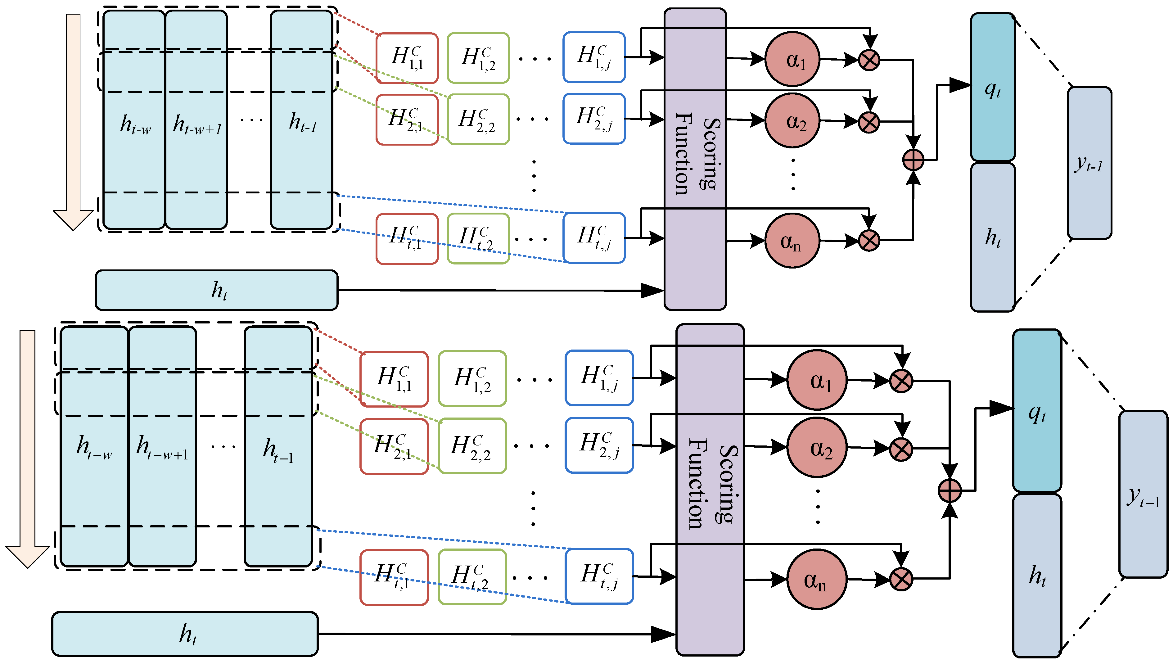
The main focus of attention mechanism [30] is to enable the network to pay attention to the most important information. In chaotic data prediction, there are many features in the input model, and the LSTM model requires a long training time during the prediction process. Moreover, traditional attention mechanisms involve comparing attention scores between two data points, which results in a high computational cost. Therefore, to fully exploit useful information in time series data, this article introduces a time pattern attention mechanism into the LSTM prediction model to deeply mine time series information from chaotic feature data. The mechanism enables a profound exploration of data information at different time steps and fully exploits important information that exists between historical data. This further improves the prediction accuracy of the LSTM model for chaotic prediction data. The structure of the time pattern attention mechanism is shown in Figure 3.

3. Build an IPSO-TPA-LSTM Chaos Data Prediction Model

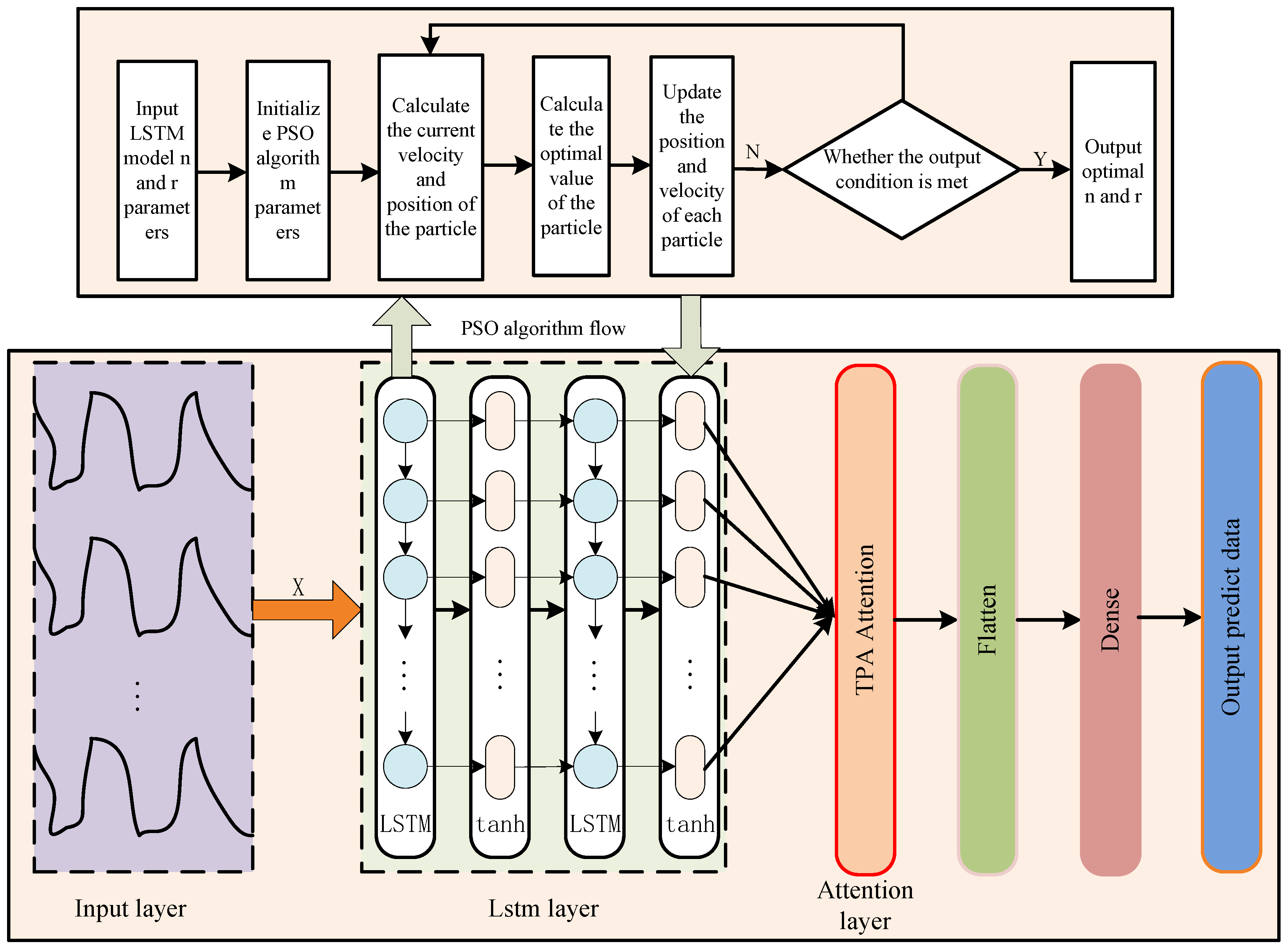
By analyzing the characteristics of chaotic data and the limitations of LSTM models in chaotic data prediction, and considering the importance of mining historical data information for prediction, this article proposes using an improved particle swarm optimization algorithm to optimize the parameters of the LSTM model and adopt a time pattern attention mechanism to deeply mine historical chaotic data information. This improves the prediction accuracy of the IPSO-TPA-LSTM model in chaotic data. The overall framework of the chaotic data prediction model is shown in Figure 4.

3.1. Input Layer

In the input layer, the input data are chaotic sequence data generated by the Lorenz system under different initial values, which are then normalized and input into the LSTM model.

3.2. LSTM Layer

In the LSTM layer, the initial parameters of the LSTM model are initialized, and the model is trained with historical chaotic data. To obtain optimal parameters (learning rate and iteration times), an improved PSO algorithm is used to optimize the parameters. The specific steps are as follows:
Step 1: Initialize chaotic data. Based on the input vector x and output vector y, determine the number of input and output neurons, and initialize the iteration times and learning rate. The aim is to balance the initial range of weights to ensure that the model can effectively learn the patterns of the data during the initial training period without causing gradient problems or training difficulties.
Step 2: Select the tanh function as the transfer function for the input layer to the hidden layer and the hidden layer to the output layer, and then calculate the hidden layer values, learning rate, and model iteration times. The purpose is to control gradient flow, better maintain internal states, and achieve the suppression and enhancement of information. This enables LSTM to excel at processing sequential data and long-term dependencies without being easily disturbed by gradient problems.
Step 3: Initialize the updated learning rate and iteration times as input of PSO, and then calculate the current particle velocity and position. The main goal of this article is to use PSO to optimize the learning rate and iteration times of the model. When the updated learning rate and iteration times of LSTM are input into the PSO model, initializing the PSO model parameters initiates the execution of the algorithm, providing a suitable starting point for the particle swarm’s search process to effectively explore the search space of the problem.
Step 4: Update the local optimal value (pbest) and global optimal value (gbest) according to the particle fitness, and calculate the updated particle velocity and position using Equation (1). Judge whether this meets the output condition. If it is met, output the optimal iteration time and learning rate; if it is not met, repeat this step. By updating local optimal values, the PSO algorithm can maintain memory during the search process, guiding particles towards more promising areas and enabling a more effective search for optimal solutions for the problem. This method helps balance global and local searches, thereby improving algorithm performance.
Step 5: Calculate the error of the optimal value of output learning rate and iteration times. If the error is less than the set value, stop calculating and output the predicted value; if the error is greater than the set value, repeat steps 2–4 until the error is met and output it. The main purpose of calculating the optimal value is to improve model performance, enhance stability and repeatability, and find the optimal combination of hyperparameters in hyperparameter adjustment to better meet the needs of machine learning tasks.

3.3. Attention Layer

Output the data from the LSTM to the attention layer, and reallocate the weights of the LSTM-predicted data to obtain the best predicted output value.

4. Chaos Data Sources

In order to fully reflect the effectiveness of the model on chaotic data prediction, the chaotic sequence data generated by a typical LORENZ system are used.

4.1. Lorenz Systems

The Lorenz system is a nonlinear three-dimensional dynamic system whose equations describe a system with complex behavior. Its chaotic behavior and strange attractor make it one of the classic examples studied in chaotic theory. The state equations of the three-dimensional Lorenz system [31] are as follows:
d x d t = δ x y d y d t = x z + r x y d z d t = x y b z
where x , y , and z represent the non-linear intensity of convective velocity, temperature difference between ascending and descending flow, and temperature distribution in the vertical direction, respectively; δ denotes the Prandtl number; r is the Rayleigh number; b denote the Shape ratio, respectively.
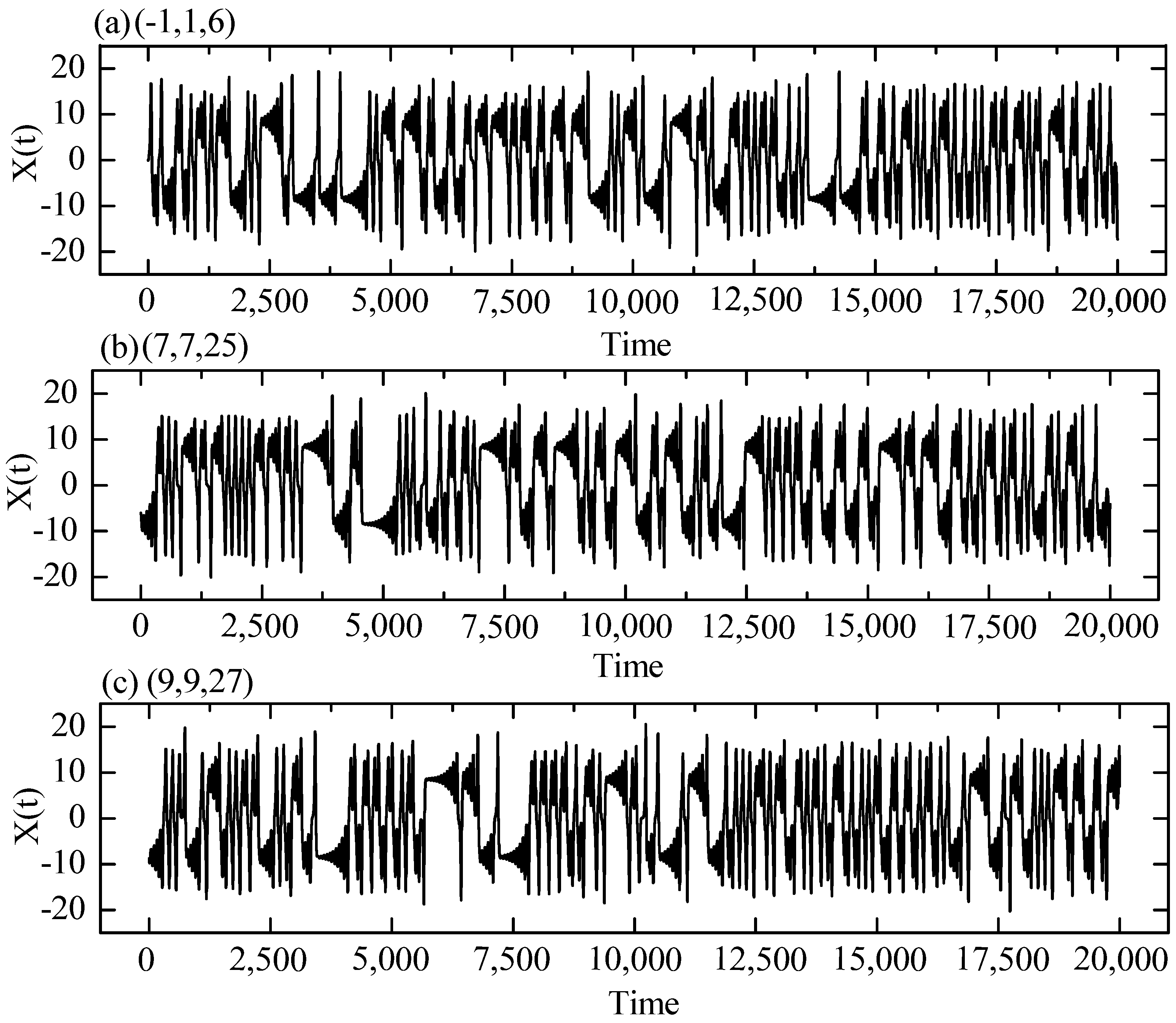
When the Lorenz system’s parameters δ, r, and b are set to 10, 8/3, and 28, respectively, the system enters a chaotic state under this set of parameters. The Lorenz system is a chaotic model with very typical characteristics. To demonstrate the strong temporal correlation of the chaotic data generated by the Lorenz system, three initial values (1, 1-1, 6), (7, 7, 25), and (9, 9, 27) were chosen to generate chaotic signal sequence plots. Due to the similarity of the data in the x, y, and z directions, the x-directional chaotic signal data were selected as an example, and the other two directions can be inferred analogously. To better demonstrate the chaotic characteristics, 100,000 generated chaotic data were screened, and the last 20,000 were selected as the example and subsequent verification model data. The x-directional sequences of the three initial values changing with time are shown in Figure 5.

4.2. Evaluation Index of the Chaotic Data Model

In order to compare the effect of different models on chaotic data prediction, using root mean square error (root mean square error (RMSE)) e R M S E , average absolute error (mean absolute error (MAE)) e M A E and goodness of fit (R2) as the evaluation index of chaotic data prediction accuracy, the smaller the value of RMSE and MAE, the better the performance of the prediction model, meaning that the value of R2 is closer to 1 and the model fitting effect is better. The model evaluation expressions are as follows:
e R M S E = 1 n i = 1 n y i y ^ i 2
e M A E = 1 n i = 1 n y i y ^ i × 100 %
R 2 = 1 i = 1 n ( y i y ^ i ) i = 1 n ( y i y ¯ i )
where n is the number of training or test samples; y ^ i is the predicted value of the chaotic data at a certain time; y ^ i is the actual measured value of the chaotic data at the same time, and y ¯ i is the average value of the data to be predicted.

5. Experimental Design and Analysis

5.1. Prediction of Chaotic Data for Different Algorithmic Models

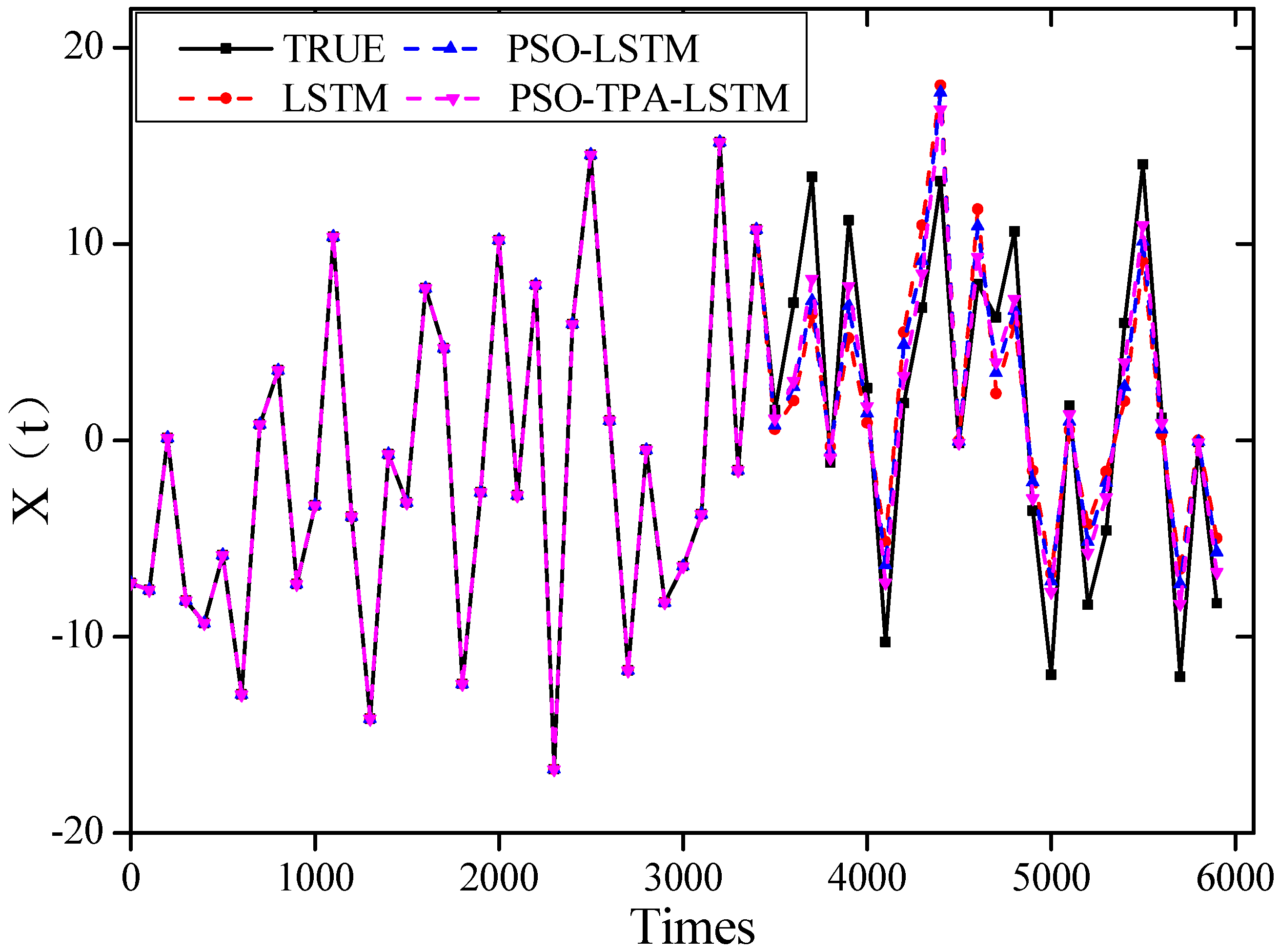
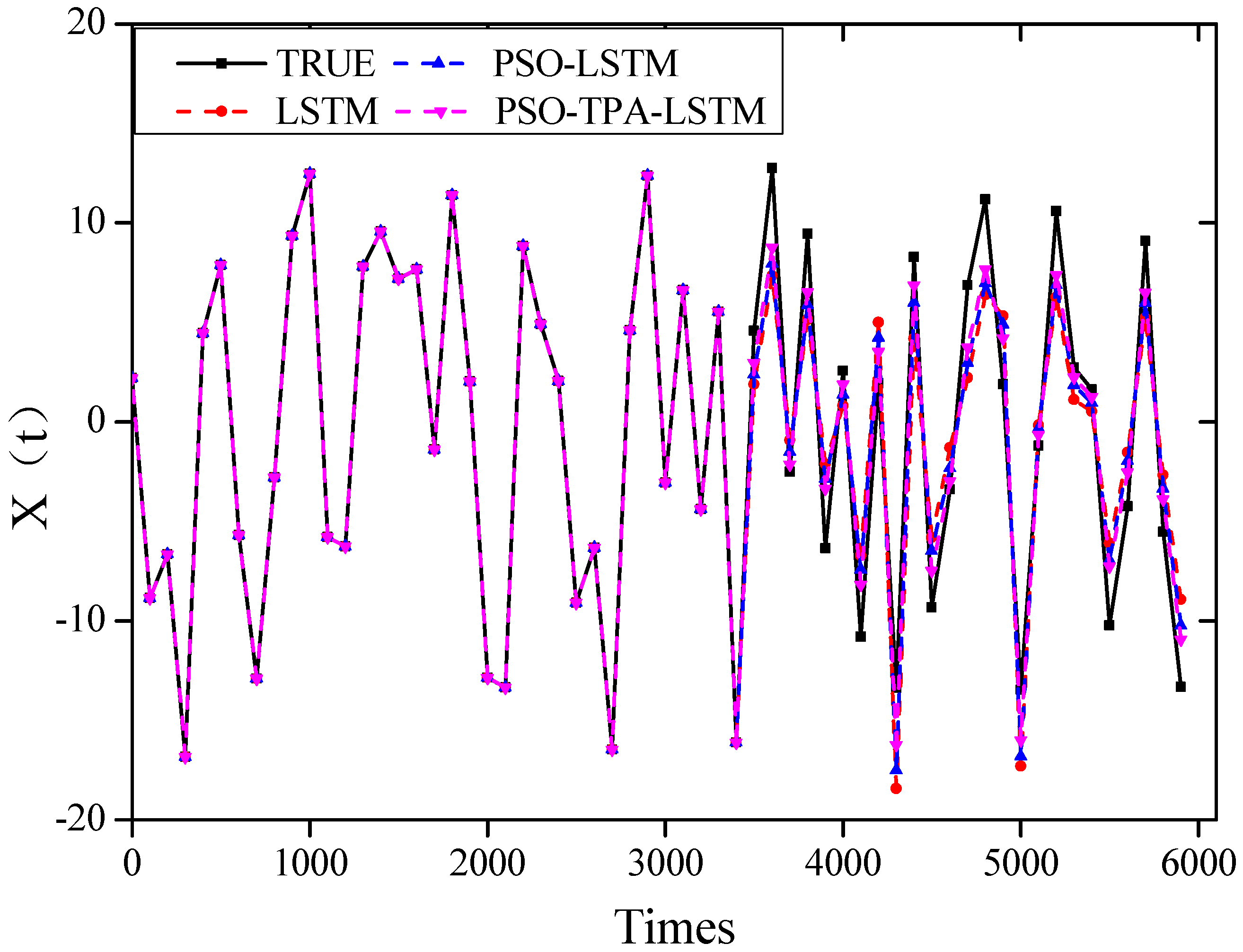
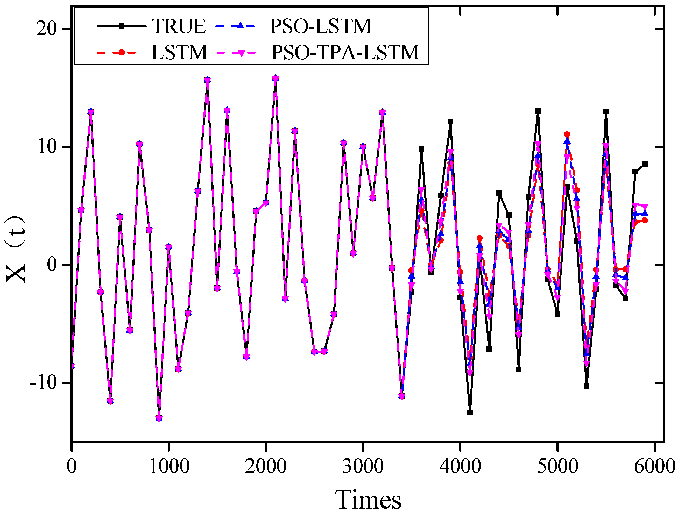
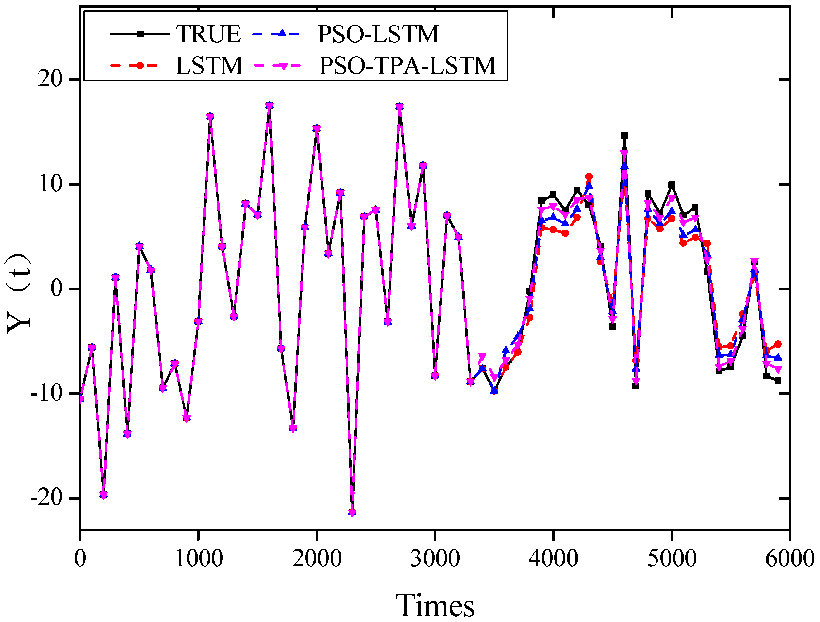
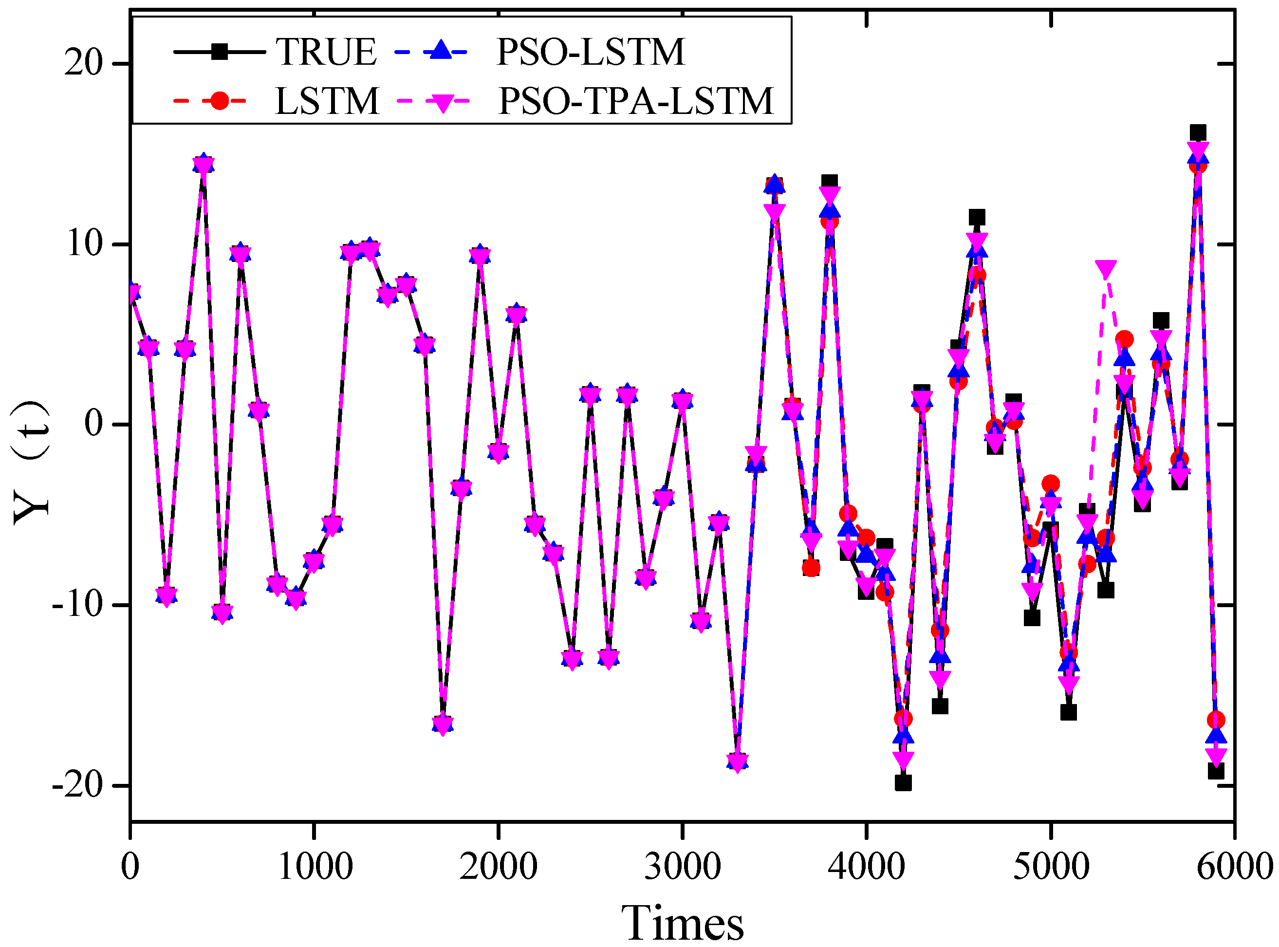
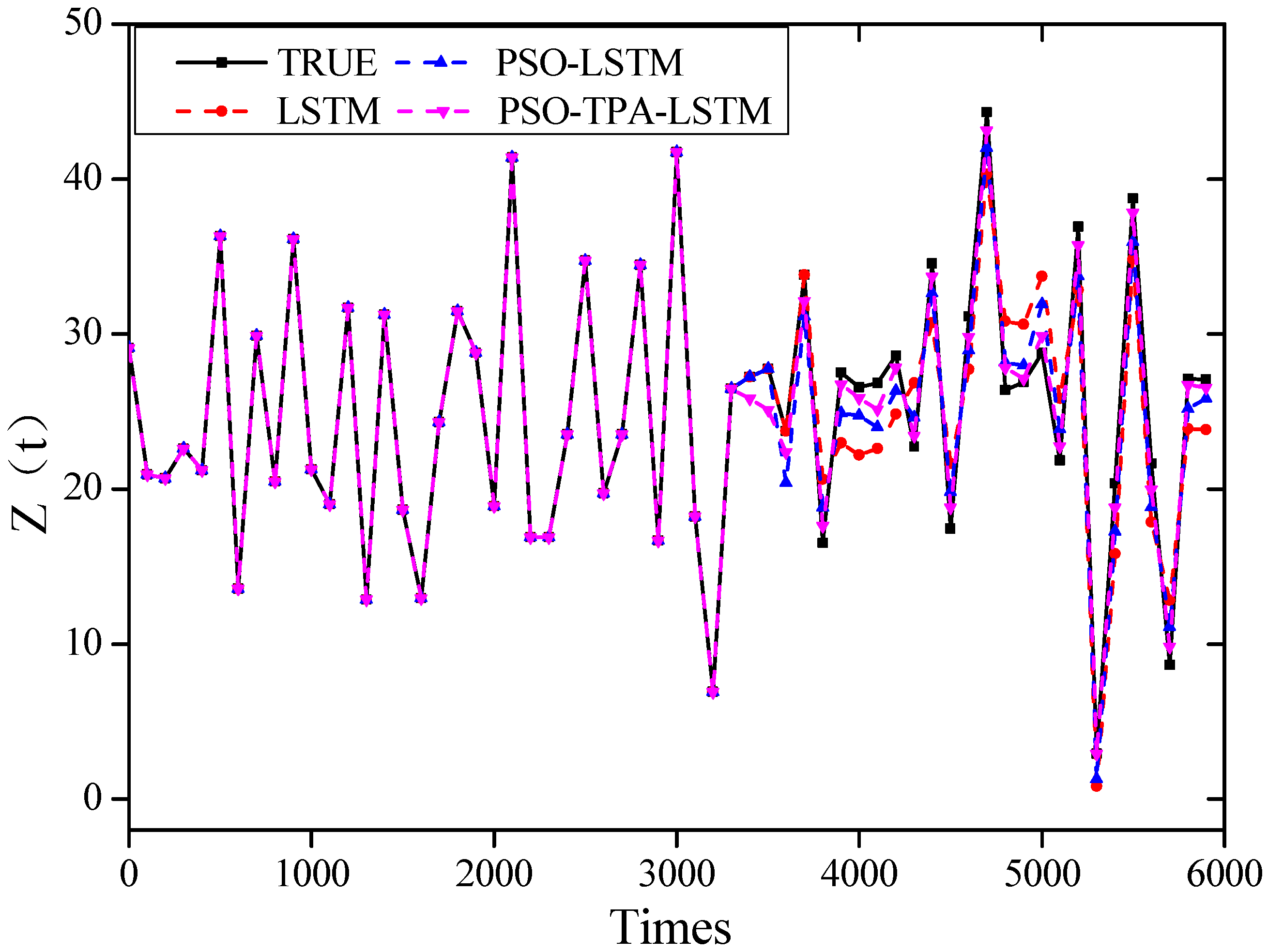
To test the effectiveness of the prediction model proposed in this article, based on the hardware configuration of Dell Inter CPU i7 and 8 GB of RAM, the simulation prediction was carried out using Python 3.7. The LSTM, PSO-LSTM prediction models and the prediction model proposed in this article were used for comparative analysis. The Lorenz system with three different initial values generated 20,000 data points in the x-direction as experimental data, and the experimental data were divided into a training set of 70% and a testing set of 30%. The prediction results are shown in Figure 6, Figure 7, Figure 8, Figure 9, Figure 10, Figure 11, Figure 12, Figure 13 and Figure 14. As can be seen from Figure 6, Figure 7, Figure 8, Figure 9, Figure 10, Figure 11, Figure 12, Figure 13 and Figure 14, the PSO-TPA-LSTM model proposed in this article has a better fitting degree in predicting the chaotic data generated from three different initial values compared to the other two models, which verifies the effectiveness of the model proposed in this article for chaotic data prediction.

5.2. Comparison of Accuracy of Different Prediction Models

The accuracy of chaotic data prediction was evaluated in this article using MAE, RMSE, and R2. The initial values (−1, 1, 6), (7, 7, 25), (9, 9, 27) Lorenz system generated XYZ three-axis chaotic data using three models (LSTM, PSO-LSTM, and PSO-TPA-LSTM), and the three index values of the models are shown in Table 1, Table 2 and Table 3. It can be seen from the tables that the evaluation indexes MAE and RMSE of the proposed PSO-TPA-LSTM prediction model are the smallest among the three different initial values generated by Lorenz system. The R2 value is closest to 1, indicating that the proposed algorithm model has the best fitting degree. MAE and RMSE measure the absolute deviation between the true value and the predicted value. The smaller their values, the smaller the absolute deviation of the model is, and the higher the prediction accuracy of the data.

6. Discussion and Conclusions

This article proposes an improved PSO-TPA-LSTM algorithm model by combining the characteristics of chaotic sequence data generated by the Lorenz system. Firstly, by adding a time attention mechanism, the key information of historical chaotic data is mined. Then, the LSTM model is used for prediction. To further improve the accuracy of LSTM model prediction, an improved particle swarm algorithm is used to optimize the parameters of the LSTM model. Finally, simulations based on Lorenz-system-generated chaotic data show that, compared to other prediction models such as LSTM and PSO-LSTM, the proposed method has higher accuracy for chaotic data prediction, providing a comprehensive reference for the prediction of chaotic-data-related industries in the future.

Author Contributions

Conceptualization, Z.C. and Q.W.; methodology, Q.W.; software, Z.C.; validation, Z.C., Q.W. and G.F.; formal analysis, Z.C.; investigation, Q.W.; resources, G.F.; data curation, Z.C.; writing—original draft preparation, Z.C.; writing—review and editing, Z.C.; visualization, Z.C.; supervision, Q.W.; project administration, Q.W.; funding acquisition, Q.W. All authors have read and agreed to the published version of the manuscript.

Funding

This research was jointly supported by the National Natural Science Foundation of China (Grant No. 41975100 and Grant No. 41775081), the Joint Research Project for Meteorological Capacity Improvement (Project No. 22NLTSZ004) and Fengyun Application Pioneering Project (Project No. FY-APP-2022.0102).

Institutional Review Board Statement

Not applicable.

Informed Consent Statement

Not applicable.

Data Availability Statement

The data presented in this study are available on request from the corresponding author. The data are not publicly available due to [It is part of author thesis work].

Acknowledgments

Author acknowledge Qiguang Wang and Guolin Feng for their technical support.

Conflicts of Interest

The authors declare no conflict of interest.

References

  1. Kumar, U.; Jain, V.K. ARIMA forecasting of ambient air pollutants (O3, NO, NO2 and CO). Stoch. Environ. Res. Risk Assess. 2010, 24, 751–760. [Google Scholar] [CrossRef]
  2. Garcia, R.C.; Contreras, J.; Van Akkeren, M.; Garcia, J.B.C. A GARCH forecasting model to predict day-ahead electricity prices. IEEE Trans. Power Syst. 2005, 20, 867–874. [Google Scholar] [CrossRef]
  3. Su, L.; Li, C. Local prediction of chaotic time series based on polynomial coefficient autoregressive model. Math. Probl. Eng. 2015, 2015, 901807. [Google Scholar] [CrossRef]
  4. Tian, Z.D.; Gao, X.W.; Shi, T. Combination kernel function least squares support vector machine for chaotic time series prediction. Acta Phys. Sin. 2014, 63, 160508. [Google Scholar] [CrossRef]
  5. Wang, S.Y.; Shi, C.F.; Qian, G.B.; Wang, W.L. Prediction of chaotic time series based on the fractional-order maximum correntropy criterion algorithm. Acta Phys. Sin. 2018, 67, 018401. [Google Scholar] [CrossRef]
  6. He, Y.; Xu, Q.; Wan, J.; Yang, S. Electrical load forecasting based on self-adaptive chaotic neural network using Chebyshev map. Neural Comput. Appl. 2018, 29, 603–612. [Google Scholar] [CrossRef]
  7. Cheng, W.; Wang, Y.; Peng, Z.; Ren, X.; Shuai, Y.; Zang, S.; Liu, H.; Cheng, H.; Wu, J. High-efficiency chaotic time series prediction based on time convolution neural network. Chaos Solitons Fractals 2021, 152, 111304. [Google Scholar] [CrossRef]
  8. Nguyen, N.P.; Duong, T.A.; Jan, P. Strategies of Multi-Step-ahead Forecasting for Chaotic Time Series using Autoencoder and LSTM Neural Networks: A Comparative Study. In Proceedings of the 2023 5th International Conference on Image Processing and Machine Vision, Macau, China, 13–15 January 2023; pp. 55–61. [Google Scholar]
  9. Yan, J.C.; Zheng, J.Y.; Sun, S.Y. Chaotic time series prediction based on maximum information mining broad learning system. Comput. Appl. Softw. 2023, 40, 253–260. [Google Scholar]
  10. Sun, T.B.; Liu, Y.H. Chaotic Time Series Prediction Based on Fuzzy Information Granulation and Hybrid Neural Network. Inf. Control 2022, 51, 671–679. [Google Scholar]
  11. Wang, L.; Wang, X.; Li, H.Q. Chaotic time series prediction model of wind power power based on phase space reconstruction and error compensation. Proc. CSU-EPSA 2017, 29, 65–69. [Google Scholar]
  12. Li, K.; Han, Y.; Huang, H.Q. Chaotic Time Series Prediction Based on IBH-LSSVM and Its Application to Short-term Prediction of Dynamic Fluid Level in Oil Wells. Inf. Control 2016, 45, 241–247, 256. [Google Scholar]
  13. Sareminia, S. A Support Vector Based Hybrid Forecasting Model for Chaotic Time Series: Spare Part Consumption Prediction. Neural Process Lett. 2023, 55, 2825–2841. [Google Scholar] [CrossRef]
  14. Wei, A.; Li, X.; Yan, L.; Wang, Z.; Yu, X. Machine learning models combined with wavelet transform and phase space reconstruction for groundwater level forecasting. Comput. Geosci. 2023, 177, 105386. [Google Scholar]
  15. Wang, H.; Zhang, Y.; Liang, J.; Liu, L. DAFA-BiLSTM: Deep Autoregression Feature Augmented Bidirectional LSTM network for time series prediction. Neural Netw. 2023, 157, 240–256. [Google Scholar] [CrossRef] [PubMed]
  16. Nasiri, H.; Ebadzadeh, M.M. MFRFNN: Multi-functional recurrent fuzzy neural network for chaotic time series prediction. Neurocomputing 2022, 507, 292–310. [Google Scholar] [CrossRef]
  17. Wang, L.; Dai, L. Chaotic Time Series Prediction of Multi-Dimensional Nonlinear System Based on Bidirectional LSTM Model. Adv. Theory Simul. 2023, 6, 2300148. [Google Scholar] [CrossRef]
  18. Huang, W.J.; Li, Y.T.; Huang, Y. Prediction of chaotic time series using hybrid neural network and attention mechanism. Acta Phys. Sin. 2021, 70, 010501. [Google Scholar] [CrossRef]
  19. Fu, K.; Li, H.; Deng, P. Chaotic time series prediction using DTIGNet based on improved temporal-inception and GRU. Chaos Solitons Fractals 2022, 159, 112183. [Google Scholar] [CrossRef]
  20. Qi, L.T.; Wang, S.Y.; Shen, M.L.; Huang, G.Y. Prediction of chaotic time series based on Nyström Cauchy kernel conjugate gradient algorithm. Acta Phys. Sin. 2022, 71, 108401. [Google Scholar] [CrossRef]
  21. Ong, P.; Zainuddin, Z. An optimized wavelet neural networks using cuckoo search algorithm for function approximation and chaotic time series prediction. Decis. Anal. J. 2023, 6, 100188. [Google Scholar] [CrossRef]
  22. Ong, P.; Zainuddin, Z. Optimizing wavelet neural networks using modified cuckoo search for multi-step ahead chaotic time series prediction. Appl. Soft Comput. 2019, 80, 374–386. [Google Scholar] [CrossRef]
  23. Jiang, P.; Wang, B.; Li, H.; Lu, H. Modeling for chaotic time series based on linear and nonlinear framework: Application to wind speed forecasting. Energy 2019, 173, 468–482. [Google Scholar] [CrossRef]
  24. Mei, Y.; Tan, G.Z.; Liu, Z.T.; Wu, H. Chaotic time series prediction based on brain emotional learning model and self-adaptive genetic algorithm. Acta Phys. Sin. 2018, 67, 080502. [Google Scholar]
  25. Awad, M. Forecasting of Chaotic Time Series Using RBF Neural Networks Optimized by Genetic Algorithms. Int. Arab. J. Inf. Technol. 2017, 14, 826–834. [Google Scholar]
  26. Long, W.; Zhang, W.Z. Parameter estimation of heavy oil pyrolysis model based on adaptive particle swarm algorithm. J. Chongqing Norm. Univ. Nat. Sci. 2023, 30, 128–133. [Google Scholar]
  27. Xu, S.B.; Xia, W.J.; Dai, A.D. A particle swarm algorithm that improves learning factors. Inf. Secur. Technol. 2012, 3, 17–19. [Google Scholar]
  28. Li, G.; Li, X.J.; Yang, W.X.; Han, D. Research on TBM boring parameter prediction based on deep learning. Mod. Tunn. Technol. 2020, 57, 154–159. [Google Scholar]
  29. Feng, Y.T.; Wu, X.; Xu, X.; Zhang, R.Q. Research on ionospheric parameter prediction based on deep learning. J. Commun. 2021, 42, 202–206. [Google Scholar]
  30. Park, J.; Jungsik, J.; Park, Y. Ship trajectory prediction based on Bi-LSTM using spectral-clustered AIS data. J. Mar. Sci. Eng. 2021, 9, 1037. [Google Scholar] [CrossRef]
  31. Lorenz, E.N. Deterministic Nonperiodic Flow. J. Atmos. Sci. 2004, 20, 130–141. [Google Scholar] [CrossRef]
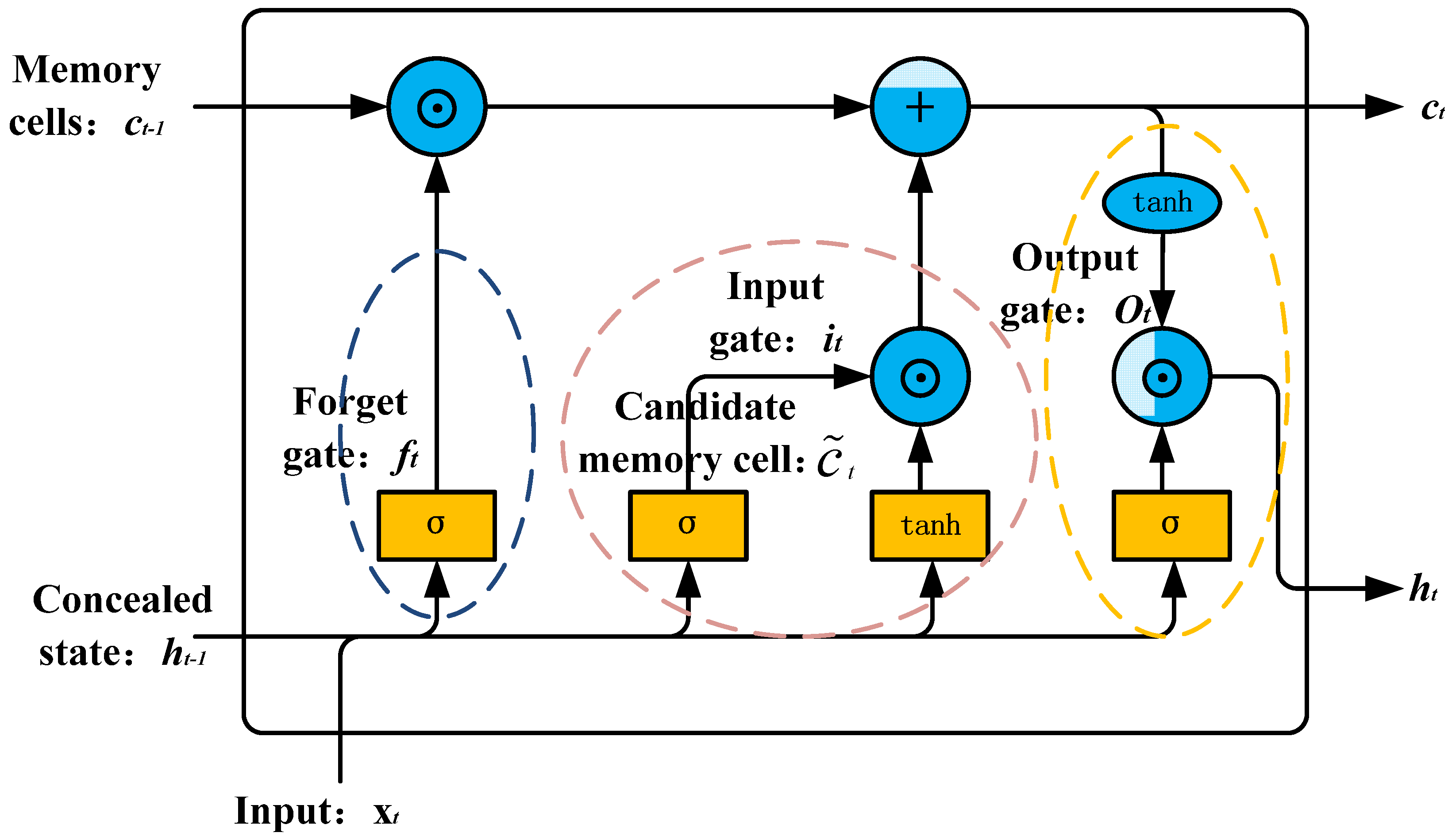
Figure 1. LSTM−cell unit’s internal structure.
Atmosphere 14 01696 g001
Figure 2. LSTM chaos data prediction model.
Atmosphere 14 01696 g002
Figure 3. Schematic representation of the mechanism structure of the temporal pattern attention.
Atmosphere 14 01696 g003
Figure 4. IPSO-TPA-LSTM model chaotic data prediction framework.
Atmosphere 14 01696 g004
Figure 5. The variation curve of X sequence (a) (1, −1, 6); (b) (7, 7, 25); (c) (9, 9, 27).
Atmosphere 14 01696 g005
Figure 6. Comparison diagram of simulation prediction of chaotic data on the X axis with initial values (−1, 1, 6).
Atmosphere 14 01696 g006
Figure 7. Comparison diagram of simulation prediction of chaotic data on the X axis with initial values (7, 7, 25).
Atmosphere 14 01696 g007
Figure 8. Comparison diagram of simulation prediction of chaotic data on the X axis with initial values (9, 9, 27).
Atmosphere 14 01696 g008
Figure 9. Comparison diagram of simulation prediction of chaotic data on the Y axis with initial values (−1, 1, 6).
Atmosphere 14 01696 g009
Figure 10. Comparison diagram of simulation prediction of chaotic data on the Y axis with initial values (7, 7, 25).
Atmosphere 14 01696 g010
Figure 11. Comparison diagram of simulation prediction of chaotic data on the Y axis with initial values (9, 9, 27).
Atmosphere 14 01696 g011
Figure 12. Comparison diagram of simulation prediction of chaotic data on the Z axis with initial values (−1, 1, 6).
Atmosphere 14 01696 g012
Figure 13. Comparison diagram of simulation prediction of chaotic data on the Z axis with initial values (7, 7, 25).
Atmosphere 14 01696 g013
Figure 14. Comparison diagram of simulation prediction of chaotic data on the Z axis with initial values (9, 9, 27).
Atmosphere 14 01696 g014
Table 1. Evaluation index data for x-axis model.
MAERMSER2
LSTM3.8742.7360.83
PSO-LSTM3.3372.6520.88
PSO-TPA-LSTM2.9832.2310.92
Table 2. Evaluation index data for y-axis model.
MAERMSER2
LSTM6.6444.38220.87
PSO-LSTM5.2613.8720.89
PSO-TPA-LSTM3.8233.5230.93
Table 3. Evaluation index data for z-axis model.
MAERMSER2
LSTM5.8374.5420.85
PSO-LSTM3.9822.9530.86
PSO-TPA-LSTM2.9832.2310.94
Disclaimer/Publisher’s Note: The statements, opinions and data contained in all publications are solely those of the individual author(s) and contributor(s) and not of MDPI and/or the editor(s). MDPI and/or the editor(s) disclaim responsibility for any injury to people or property resulting from any ideas, methods, instructions or products referred to in the content.