A Survey of Deep Learning-Based Lightning Prediction

Abstract

The escalation of climate change and the increasing frequency of extreme weather events have amplified the importance of precise and timely lightning prediction. This predictive capability is pivotal for the preservation of life, protection of property, and maintenance of crucial infrastructure safety. Recently, the rapid advancement and successful application of data-driven deep learning across diverse sectors, particularly in computer vision and spatio-temporal data analysis, have opened up innovative avenues for enhancing both the accuracy and efficiency of lightning prediction. This article presents a comprehensive review of the broad spectrum of existing lightning prediction methodologies. Starting from traditional numerical forecasting techniques, the path to the most recent breakthroughs in deep learning research are traversed. For these diverse methods, we shed light on their progression and summarize their capabilities, while also predicting their future development trajectories. This exploration is designed to enhance understanding of these methodologies to better utilize their strengths, navigate their limitations, and potentially integrate these techniques to create novel and powerful lightning prediction tools. Through such endeavors, the aim is to bolster preparedness against the growing unpredictability of climate and ensure a proactive stance towards lightning prediction.

1. Introduction

Weather fluctuations have long been an unpredictable force, and humankind’s desire to control such atmospheric caprice dates back to antiquity. Cinematic depictions such as in the “Thor” franchise often portray weather manipulation, particularly lightning, as a profound testament to power. The immense destructive force associated with lightning encapsulates its menacing presence in collective consciousness. Presently, no effective mechanisms exist to prevent or mitigate the intensity of lightning, rendering lightning prediction an imperative field of study. Since the 1950s, technological advancements encompassing computers, radar, lasers, remote sensing, and artificial satellites have catalyzed meteorological developments, significantly enhancing capabilities in lightning prediction.

Global satellite data indicates approximately 46 lightning strikes occurring every second across the globe, leading to over 10,000 fatalities and economic damages exceeding one billion USD annually. In response to these sobering statistics, a holistic meteorological monitoring system has been instituted, integrating atmospheric background stations, climate observatories, terrestrial automated meteorological stations, high-altitude meteorological stations, next-generation weather radars, and meteorological satellites. This amalgamation of technologies provides a comprehensive framework for lightning observations.

Traditional lightning prediction methodologies primarily pivot on the monitoring of atmospheric parameters and meteorological phenomena. By interpreting weather data, these approaches identify meteorological conditions conducive to lightning. Numerical model prediction, underpinning most traditional lightning forecasting methods, exploits principles from atmospheric dynamics, thermodynamics, and related fields to formulate models that simulate atmospheric processes. However, the accuracy of these models requires enhancement due to the complex multi-scale physical processes implicated in lightning.

The advent of data-driven machine learning and the conceptualization of deep learning, proposed by Hinton et al. in 2006 [1], spurred the rapid evolution of machine learning methods. Deep learning, a subfield of machine learning, comprises multilayer perceptions (MLP) [2], with its primary objective being to mimic the workings of the human brain. It strives to learn data representation techniques, encompassing inherent data correlations, to attain a level of cognitive processing comparable to the human brain, thereby endowing machines with human-like learning and analytical capabilities [3].

Deep learning employs artificial neural networks (ANN) [4] for data learning and representation. Characterized by multiple layers, it represents data at varying levels of abstraction, hence capturing intricate data patterns and structures. Neurons, the basic computational units of deep learning, simulate certain functionalities of biological neurons. The input layer accepts raw data, the hidden layer extracts features and processes information, and the output layer delivers the final prediction. Forward propagation begins with the input layer feeding data into the neural network, progressing towards the output layer, computing layer by layer to yield prediction results. The accuracy of these results is evaluated using a loss function, such as mean squared error or cross-entropy. A smaller loss function indicates superior prediction performance. The loss function is minimized via backpropagation, an optimization algorithm based on gradient descent. To boost the model’s generalization capabilities, regularization strategies and optimization algorithms can be integrated into the neural network training process.

With Professor Hinton’s team securing the championship in the 2012 ImageNet image recognition competition with their deep neural network [5], deep learning began to supersede traditional machine learning algorithms across many domains, emerging as a sought-after research direction within artificial intelligence. Deep learning is widely utilized in areas such as computer vision and time-series data prediction, extending its reach to lightning prediction.

This article aims to provide a thorough review of lightning prediction methodologies. It begins with a fundamental understanding of lightning prediction principles, delves into traditional numerical prediction methods, explores lightning prediction through conventional machine learning, and then delves deeply into the crux of the article—deep learning-based lightning prediction, which currently dominates lightning prediction research. This includes the exploration of recurrent neural networks, convolutional neural networks, and hybrid neural network methodologies. The final section encapsulates the salient features of the discussed methodologies and envisages future trends in deep learning-based lightning prediction.

2. Numerical Prediction Methods

Numerical prediction methodologies for forecasting lightning occurrences are grounded in the mechanisms governing lightning generation. Typically, these methodologies utilize parameterization schemes within the Weather Research and Forecasting (WRF) model. Serving as a versatile meteorological prediction tool, the WRF model encompasses numerous applications, ranging from real-time numerical weather prediction (NWP) and weather event research to the development of simulation models and parameterized physics. Additionally, it contributes to studies of regional climate simulations, air quality modeling, atmosphere–ocean coupling, and idealized atmospheric research [6]. The WRF model houses four critical lightning parameters, employed for estimating the Lightning Potential Index (LPI) and the frequency of lightning events. These parameters serve as key indicators in predicting the possibility and the frequency of lightning occurrence, thereby contributing significantly to the field of meteorological prediction and research.

LPI: LPI [7] is defined as the volume integral of the total mass flux of liquid water and ice in the “charging zone” (0 ${}^{\circ }$C to −20 ${}^{\circ }$C) within a thundercloud. It typically represents the likelihood of a thundercloud separating electric charges through the latent ice pellet mechanism. LPI varies over time, as it is estimated from the kinematic and microphysical model fields at each grid point and time step. In short, LPI measures the likelihood of charge generation and separation during lightning initiation. The basic formula is as follows:

$$LPI=\frac{1}{V}\int \int \int \epsilon w^{2}dxdydz$$

(1)

where V represents the cloud volume in the “charging zone”, w denotes the vertical wind component (ms${}^{-1}$), and $\epsilon$ is a dimensionless number that depends on the mixing ratio of hydrometeor components, ranging from 0 to 1. The main data considered are the mixing ratios of cloud ice, snow, and graupel.

Lightning frequency: Price and Rind (1992, PR92) [8] developed a simple parameterization to simulate the global distribution of lightning. As lightning activity in convective clouds is positively correlated with the intensity of updrafts, and the intensity of updrafts is related to cloud top height, different lightning parameters were established for continental and oceanic storms due to the differences in their cloud characteristics. In both cases, convective cloud top height is considered as a variable. The parameterization for continental storms is defined as follows:

$$F_c=3.44\times {10}^{-5}{H}^{4.9}$$

(2)

$$w_c=1.49H^{1.09}$$

(3)

In this case, $F_c$ represents the continental lightning frequency (in lightning strikes per minute), H is the height of the convective cloud top, and $w_c$ is the maximum updraft strength. The lightning parameterization for oceanic convective clouds follows a similar form, which is:

$$F_m=6.4\times {10}^{-4}{H}^{1.73}$$

(4)

$$w_m=2.86H^{0.38}$$

(5)

Price and Rind (1993, PR93) [9] used radiosonde data collected from 17 observation stations in the western United States to perform lightning predictions. PR93 primarily focused on two parameters in lightning: the freezing level height ($H_0$) and the cold cloud thickness $dH$ (the thickness from 0 ${}^{\circ }$C to the cloud top, which is $dH=H_{top}-H_0$). The proportion Z is derived from the parameterization of the total flash (IC + CG) frequency and the observed cloud-to-ground flash frequency.

$$Z=0.021{\left(dH\right)}^4-0.648{\left(dH\right)}^3+7.49{\left(dH\right)}^2-36.54dH+63.09$$

(6)

Price and Rind (1994, PR94) [10] introduced the calibration factor parameter, specifically on latitude, longitude, and season. They used the global convective cloud data from 1983 to 1990 at 3 h intervals provided by the International Satellite Cloud Climatology Project. By studying different grid sizes, they reached the following conclusions (lightning at a 5 km${}^2$ resolution divided by lightning at a lower resolution):

$$c=0.97241\exp \left(0.048203R\right)$$

(7)

where c represents the calibration factor and R is the grid area in squared degrees.

Lynn et al. modified the original LPI to predict the hourly lightning flash density [11]. They have made the LPI adaptable for grid scales from 1 to 4 km. Case studies confirm its applicability on both ultra-high resolution (1.33 km) and high-resolution (4 km) grids. Gharaylou et al. examined the performance of potential difference (POT) and LPI in predicting lightning activity [12]. Derived from the WRF model, LPI showed superior predictive accuracy compared to POT, which uses the ELEC model package. Analyzing a decade of Tehran data, both indices matched actual lightning locations, with LPI being more precise. However, the simulated lightning flash count did not correlate significantly with WWLLN (The World Wide Lightning Location Network) data, possibly due to the absence of WWLLN observatories in the area.

3. Traditional Machine Learning Methods

Machine learning harnesses computational learning methodologies to augment system performance through experiential learning. This technology equips machines with the capability to discern patterns within complex datasets and to predict prospective behaviors, outcomes, and trends [13]. Traditional machine learning algorithms encompass decision trees (DT) [14], support vector machines (SVM) [15], random forests (RF) [16], naive Bayes [17], and simple ANNs. These methods are heavily reliant on manual feature extraction, with the manual construction of features being an essential component when employing these traditional machine learning algorithms in lightning prediction.

Azad et al. put forth a hybrid model aiming to predict the monthly frequency of lightning occurrences [18]. This model commences with a random forest to sieve out 11 impactful predictive features from a pool of 21 feature parameters obtained from 28 observation stations of the Bangladesh Meteorological Department ranging from 1981 to 2016, including the convective rain rate, Earth skin temperature, monthly averaged precipitation, and so on. Subsequently, the ensemble empirical mode decomposition (EEMD) [19] is deployed to deconstruct the original time-series data into a finite set of intrinsic mode functions (IMF) [20] and residuals. Irrelevant or redundant IMFs and residuals are discarded, with the selection of IMFs primarily being those that have a higher frequency band and display a significant correlation with the original sequence. These chosen IMFs, combined with other input parameters, serve as inputs to the ANN or SVM models. These models are then used to construct a predictive model for the frequency of lightning occurrences. This approach integrates the strengths of multiple techniques to increase the accuracy and robustness of lightning frequency prediction. The ANN adopts a backpropagation (BP) neural network, and its model mechanism is as follows:

$$y\left(x\right)=\sum _{j=1}^n{w}_j\left(p\right)x_j\left(p\right)+c$$

(8)

The mechanism of the SVM model is as follows:

$$L\left(m,m_j\right)=exp(-\frac{\left(\right||m-m_j^2|\left|\right)}{2{\phi }^2})$$

(9)

In order to evaluate model performance, the authors introduced a coefficient $R^2$ of determination, which is defined as follows:

$$R^2=1-\frac{{\sum }_{i=1}^N{({\delta }_t-{\widehat{\delta }}_t)}^2}{{\sum }_{i=1}^N{({\delta }_t-{\overline{\delta }}_t)}^2}$$

(10)

where ${\delta }_t$ represents the reference values, ${\widehat{\delta }}_t$ represents the predicted values at time t, and ${\overline{\delta }}_t$ denotes the mean of the reference values, simultaneously using the root-mean-square error (RMSE), mean absolute error (MAE), mean absolute percentage error (MAPE), index of agreement (IA), and sensitivity analysis to validate the input parameters and consistency of results. In particular their model showed 8.02–22.48% higher performance precision in terms of RMSE compared to other models.

Schön et al. proposed an innovative approach to lightning prediction that utilizes prediction errors derived from lightning forecasting models [21]. Traditional forecasting models for lightning generally rely on predictions of specific physical parameters, such as temperature and humidity. However, these models often face difficulties in accurately predicting the timing and location of lightning events. To address this issue, the authors have introduced a new methodology that employs prediction errors of lightning forecasting models as features. The input consists of two data sources: binary meteosat satellites images for different channels and lighning-detected data. Machine learning algorithms are then utilized to predict lightning occurrences. The authors argue that these prediction errors encompass substantial information regarding atmospheric conditions and other influential factors, which could be pivotal in predicting the timing and location of lightning events. In their experiments, a machine learning model was developed based on the gradient boosting algorithm. This model used prediction errors and other relevant meteorological data to enhance the accuracy of lightning prediction up to 96% for predictions over the next 15 min and above 83% for the next five hours.

Pakdaman et al. employed a simple ANN and a decision tree as two binary classification algorithms to predict lightning occurrences [22]. They used parameters collected from historical data (1992–2018) of three synoptic weather stations, including cloud cover, wind direction, wind speed, dry temperature, dew point, and so on. Due to the imbalance in the acquired source data, undersampling techniques were initially applied to rectify this issue, resulting in several balanced data subsets. These subsets were then input into a shallow neural network (with one hidden layer) and a decision tree, respectively, for classification predictions. The prediction results were evaluated based on metrics such as precision, recall, accuracy, and F-measure, with the model based on a simple ANN achieving results above 0.5 and the model based on DT achieving results above 0.85. Johari et al. proposed a simple ANN to predict the occurrence of lightning and also used meteorological parameters, such as wind, dew point, humidity, pressure, temperature, cloud height, and moisture difference, as input features [23]. A two layer back-propagation neural network was developed to predict the occurrence of lightning at least four hours prior to its arrival. Through continuous training and adjusting the activation functions and network structure, a network with high accuracy and convergence capability was achieved. RMSE was used to evaluate the accuracy of developed network, with a value of 0.41% being achieved, and a regression coefficient up to 0.99997. Moon S. H. and colleagues employed machine learning techniques, specifically SVM and RF, to predict the likelihood of lightning occurrences within specific locations and time intervals [24]. Their data were sourced from the European Centre for Medium-range Weather Forecasts, including 112 weather variables, such as temperature, wind speed, relative humidity, and convective available potential energy, focusing on the Korean Peninsula region. To enhance prediction accuracy, they undersampled the data points that were not linked with lightning events and computed the probability of detection (POD), the false-alarm ratio (FAR), and the equitable threat score (ETS) as performance criteria, with threat scores of 0.0885 and 0.0828 for SVM and RF. The ETS of results from SVMs could be increased to 0.1241 if the temporal resolution was reduced by a factor of 2 and 0.1499 if the spatial resolution was reduced by a factor of 3.

$$POD=\frac{TP}{TP+FN}$$

(11)

$$FAR=\frac{FP}{TP+FP}$$

(12)

$$ETS=\frac{TP-\alpha }{TP+FP+FN-\alpha }$$

(13)

where $\alpha$ denotes teh proportion of correct forecasts expected by chance alone:

$$\alpha =\frac{(TP+FP)(TP+FN)}{TP+FP+FN+TN}$$

(14)

Overall, traditional machine learning methods have been shown to offer significantly greater accuracy and efficiency than conventional lightning prediction methodologies. These methods primarily revolve around constructing features from lightning observation data, which often necessitates specialized knowledge. In this respect, deep learning holds a significant advantage due to its capacity to learn and extract meaningful features from complex datasets autonomously.

4. Deep Learning Methods

4.1. Convolutional Neural Network Methods

Convolutional neural networks (CNNs) represent a specialized category of feedforward neural networks characterized by their convolutional computations and deep structures. CNNs possess the ability to extract features directly from raw data, obviating the need for complex preprocessing, thereby finding extensive application in the field of computer vision. The distinctiveness of CNNs lies in two facets: first, the lack of full connectivity between neurons; second, the sharing of weights across neurons within the same layer. This configuration of partial connectivity and weight-sharing brings CNNs closer to the functioning of biological neural networks, effectively reducing both the complexity of the network model and the number of weights [25].

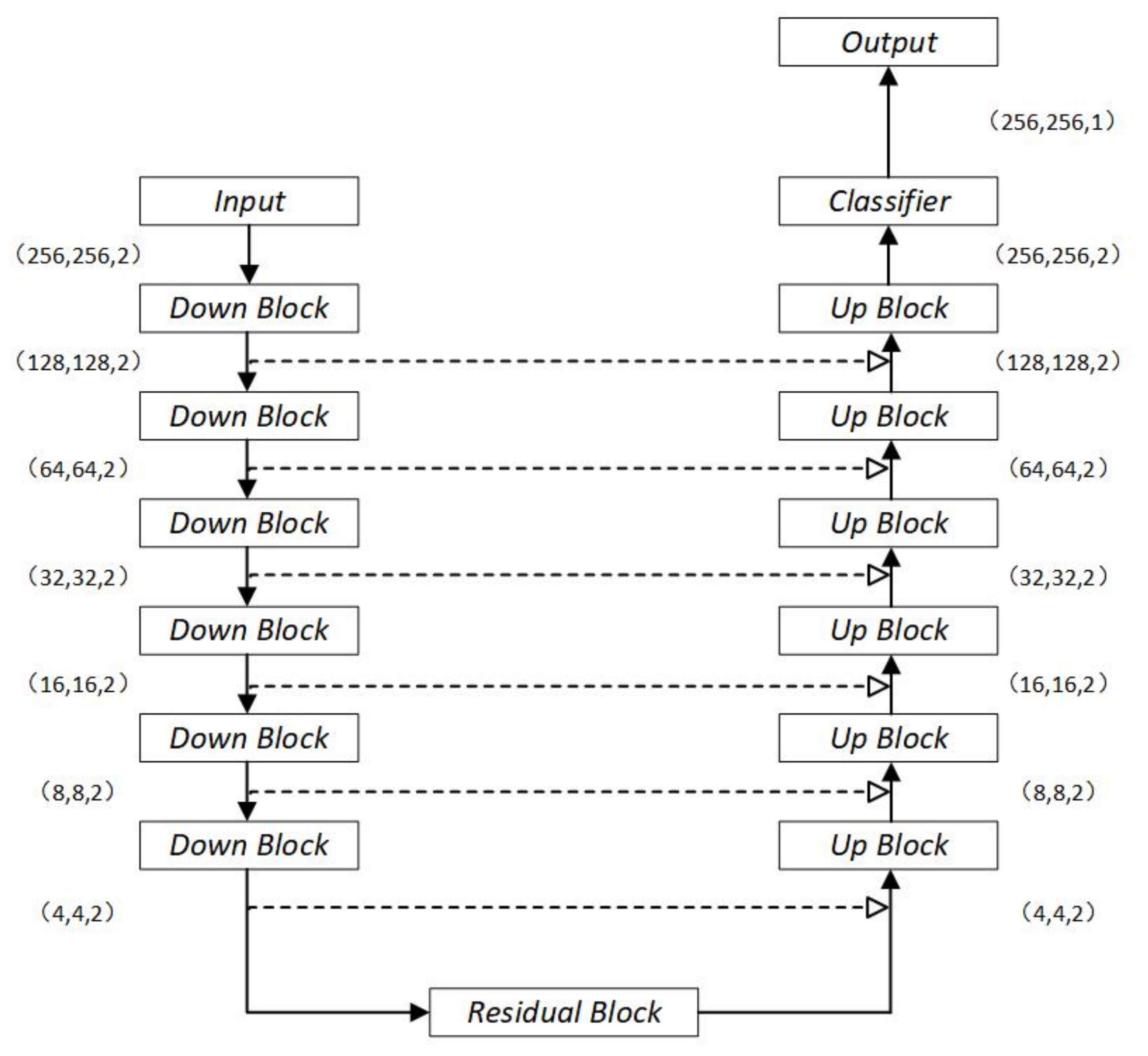
In modern meteorological systems, geostationary satellites hold a pivotal role, with satellite images often serving as a common medium for lightning prediction. A noteworthy example of this can be seen in the work of Sebastian Brodehl et al., who proposed an end-to-end CNN-based lightning prediction method that employs geostationary satellite images [26]. This approach allows for the direct prediction of lightning events from satellite images. The network architecture is underpinned by U-Net [27] and complemented by ResNet-v2 [28] residual blocks, adapted to handle three-dimensional input encompassing the height and width of an image, along with time frames. In this model, stacked convolution layers and the pooling layer at each down/up-sampling step are replaced with residual blocks. While convolutions are used for down-sampling, deterministic trilinear up-sampling operations are implemented. Batch normalization layers are supplanted with instance normalization, and instead of cropping the feature map of the contracting path, the feature map post the down-sampling operation is used. The model, demonstrated in Figure 1, maintains a fixed height and width of 256 × 256 px and is capable of handling imbalanced data without any requirement for pre-processing. Most information is drawn from structures in the visible spectrum, with infrared imaging providing some degree of classification performance during night-time. Furthermore, an attention mechanism-based enhanced model is proposed, which more effectively captures the spatio-temporal features of lightning events, thereby improving prediction accuracy and interpretability. The authors evaluated the performance by calculating the critical success index (CSI) at decreased lead times, with more values greater than 99% for 0 min, 87% for 30 min, and 24% for 180 min.

$$CSI\left(\mathrm{\Omega }\right)=\frac{{\sum }_{s\in \mathrm{\Omega }}TP\left(s\right)}{{\sum }_{s\in \mathrm{\Omega }}TP\left(s\right)+{\sum }_{s\in \mathrm{\Omega }}FN\left(s\right)+{\sum }_{s\in \mathrm{\Omega }}FP{\left(s\right)}^{\prime }}$$

(15)

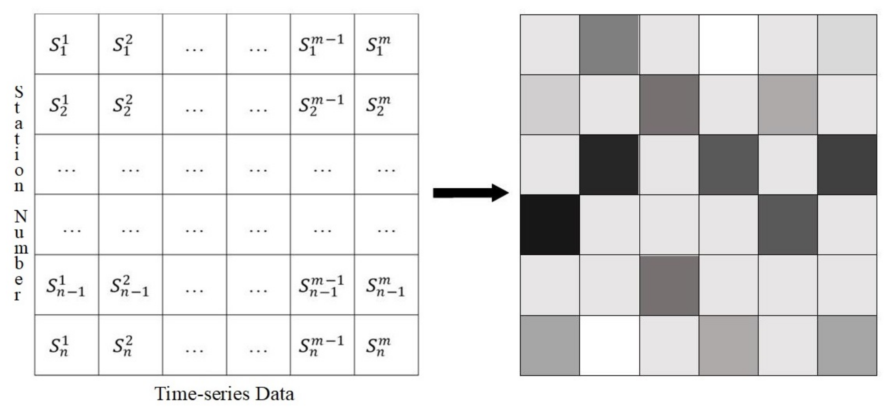
To accommodate time-series data as input for CNNs, Bao et al. conducted feature reconstruction on time-series atmospheric electric field observation data [29]. The time-series observation data were treated as the horizontal coordinate and the observation sites as the vertical coordinate, forming a two-dimensional image as depicted in Figure 2. A straightforward three-layer network was utilized to convert the time-series data into image data, with the sigmoid activation function transforming the original data into a range of 0–1. The KL divergence [30] was integrated as a penalty mechanism in this process. The visualized data thus produced was used as input for the CNN, which was based on an enhanced ResNet50 architecture. The main branch employed 3 × 3 convolutional kernels for down-sampling, while the shortcut branch incorporated a 2 × 2 max-pooling layer. This network could discern between lightning and non-lightning weather. In instances of a lightning event, the location of the lightning could be determined using an MLP, which comprises an input layer, multiple hidden layers, and an output layer. The MLP, primarily used for the classification and prediction of nonlinear relationships, took the spatial position of the lightning as its input and produced the impending lightning location as its output. The mean square error (MSE) was used as the evaluation index for model training, while the negative log likelihood (NLL) loss was used for classification. The performance of the method yields satisfactory results, with 88.2% accuracy, 92.2% precision rate, 81.5% recall rate, and 86.4% F1-score.

In their study, Sashiomarda et al. leveraged electromagnetic and acoustic signals from lightning in tandem with a CNN to predict the precise location of lightning events [31]. They converted a medley of random noise, lightning sounds, and background noise into spectrograms and subsequently sectioned these into a multitude of millisecond-scale audio signals. Each of these slices underwent a discrete Fourier transform, a process that was also applied to the electromagnetic signals emanating from the lightning. These transformed spectrograms served as inputs for the CNN, which utilized max-pooling and ReLU activation functions. The culmination of this process yielded three distinct categories: “quiet”, “unknown”, and “lightning”. By pinpointing the origin of the detected sounds, the researchers were able to determine not only the occurrence of a lightning event but also its exact location. Their method of lightning prediction achieved high scores of up to 99%.

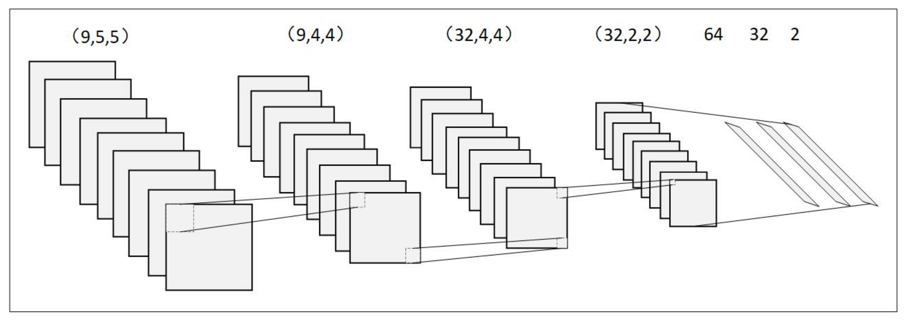
Lu et al. used 3D weather radar data to predict the location of lightning strikes [32]. They used a M × N sliding window to obtain radar data samples, one of which contains nine layers. If the lightning data point were located in the center grid of the sliding window, it was considered that the lightning occurred in that area; otherwise, it did not. In this way, predicting the location of lightning became a binary classification problem. They used methods such as CNN, logistic regression [33], random forest, and k-nearest neighbors [34] for prediction. Among them, the CNN performed the best. The structure of the CNN is shown in Figure 3. The CNN consists of seven layers, with two convolutional layers and two pooling layers appearing alternately. There were three fully connected (FC) layers connected to the last feature map. The results showed that the CNN has best performance in predicting the lightning strike locations with a precision of 0.842, an FPR (false-positive rate) of 0.158, a recall of 0.604, accuracy of 0.967, ROC AUC([35]) of 0.798, and P–R(precision–recall) of 0.534.

4.2. Recurrent Neural Network Methods

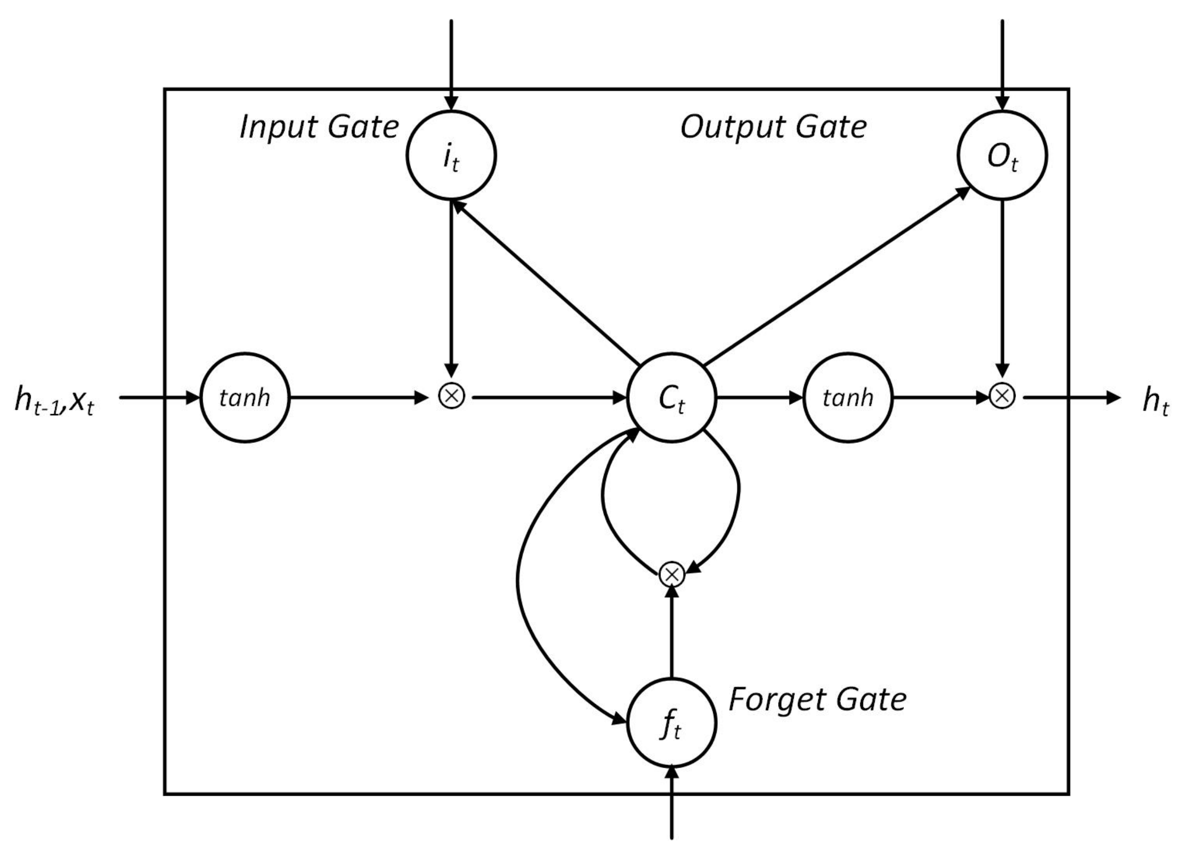
Recurrent neural networks (RNNs) are a type of recursive neural network specifically designed to process sequence data. They accomplish this by iteratively processing the sequence in a sequential direction, with all nodes (or recurrent units) connected in a chain-like pattern. The unique trait of RNNs is that their input comprises not only the current data but also information from previous steps. When it comes to lightning prediction, RNNs often employ long short-term memory (LSTM) networks. LSTMs were created to tackle the challenge of long-term dependencies often encountered in standard RNNs [36], shown in Figure 4. By feeding the spatio-temporal features of lightning data into the LSTM, reliable lightning predictions can be made. Presently, LSTM is the most frequently used deep learning network model for lightning prediction.

Bao et al. employed a spatio-temporal localization method leveraging LSTM neural networks and interpolation techniques to predict and monitor lightning activity [37]. The team utilized time-series data captured from 30 atmospheric electric field instruments as LSTM input, with a softmax function categorizing the results into five classes to predict lightning timing. In order to predict the location of the lightning, they enhanced the prediction accuracy by incorporating data from multiple networked atmospheric electric field instruments. They also employed the ordinary kriging (OK) interpolation method [38]—one of the most commonly used kriging methods—to derive the electric potential distribution and infer the likely area of impending lightning. By integrating these two methodologies, they achieved satisfactory prediction outcomes, with a POD of 89.08%, FAR of 15.85%, and CSI of 76.82%.

Fukawa et al. proposed a novel method for lightning prediction using direct electric field data [39]. They collected data in both fair weather and lightning weather as the input of their many-to-one network. This network model was based on LSTM, and the specific network structure is shown in Figure 5. MAPE was applied to measure accuracy, and the anomaly score $\alpha$ was used to control the output. If, in fair weather, $\alpha$ was 0, it should be exposed to sudden changes in the case of lightning. The electric field sum $\beta$ was intended to accurately predict the electric field value in fair weather. It was confirmed that 88.9% of lightning occurred while alarming.

$$MAPE=\frac{100}{n}\sum _{n=1}^n\left|\frac{{\widehat{v}}_i-v_i}{v_i}\right|$$

(16)

$$\alpha ={log}_2\left(\sum _i^{i+300}\left|\widehat{v}-v\right|\right)$$

(17)

$$\beta ={log}_2\left(\sum _i^{i+300}\left|v\right|\right)$$

(18)

Extending upon the popular fully connected LSTM architecture, Shi et al. introduced a convolutional LSTM (ConvLSTM) model, primarily to cater to spatio-temporal data features [40]. The ConvLSTM model morphs the 2D input in LSTM into a 3D tensor, with the last two dimensions symbolizing spatial dimensions (rows and columns). For data at each time instance ‘t’, ConvLSTM replaces certain connection operations in LSTM with convolution operations. This implies that ConvLSTM predictions are based on the current input and the past states of its local neighbors. In ConvLSTM, $X_1$…$X_t$ represent inputs, $C_1$…$C_t$ represent cell outputs, and $H_1$…$H_t$ represent hidden outputs. $g_t$, $i_t$, and $f_t$ represent the three gates and are three-dimensional tensors, with the last two dimensions being spatial components. The calculation formulas for the outputs of each layer and the related gates are as follows:

$$g_t=tanh(W_{xg}\ast X_t+W_{hg}\ast H_{t-1}+b_i)$$

(19)

$$i_t=\sigma (W_{xi}\ast X_t+W_{hi}\ast H_{t-1}+W_{ci}\circ C_{t-1}+b_i)$$

(20)

$$f_t=\sigma (W_{xf}\ast X_t+W_{hf}\ast H_{t-1}+W_{cf}\circ C_{t-1}+b_f)$$

(21)

$$C_t=f_t\circ C_{t-1}+i_t\circ g_t$$

(22)

$$o_t=\sigma (W_{xo}\ast X_t+W_{ho}\ast H_{t-1}+W_{co}\circ C_t+b_c)$$

(23)

$$H_t=o_t\circ tanh\left(C_t\right)$$

(24)

where $\sigma$ represents the sigmoid activation function, ∗ denotes the convolution operation, and ∘ signifies the Hadamard product. The input gate $i_t$, forget gate $f_t$, output gate $o_t$, and input modulation gate $g_t$ control the flow of information in the memory cell $C_t$. They obtained good performance, with a Rainfall-MSE of 1.420, CSI of 0.577, FAR of 0.195, POD of 0.660, and correlation of 0.908.

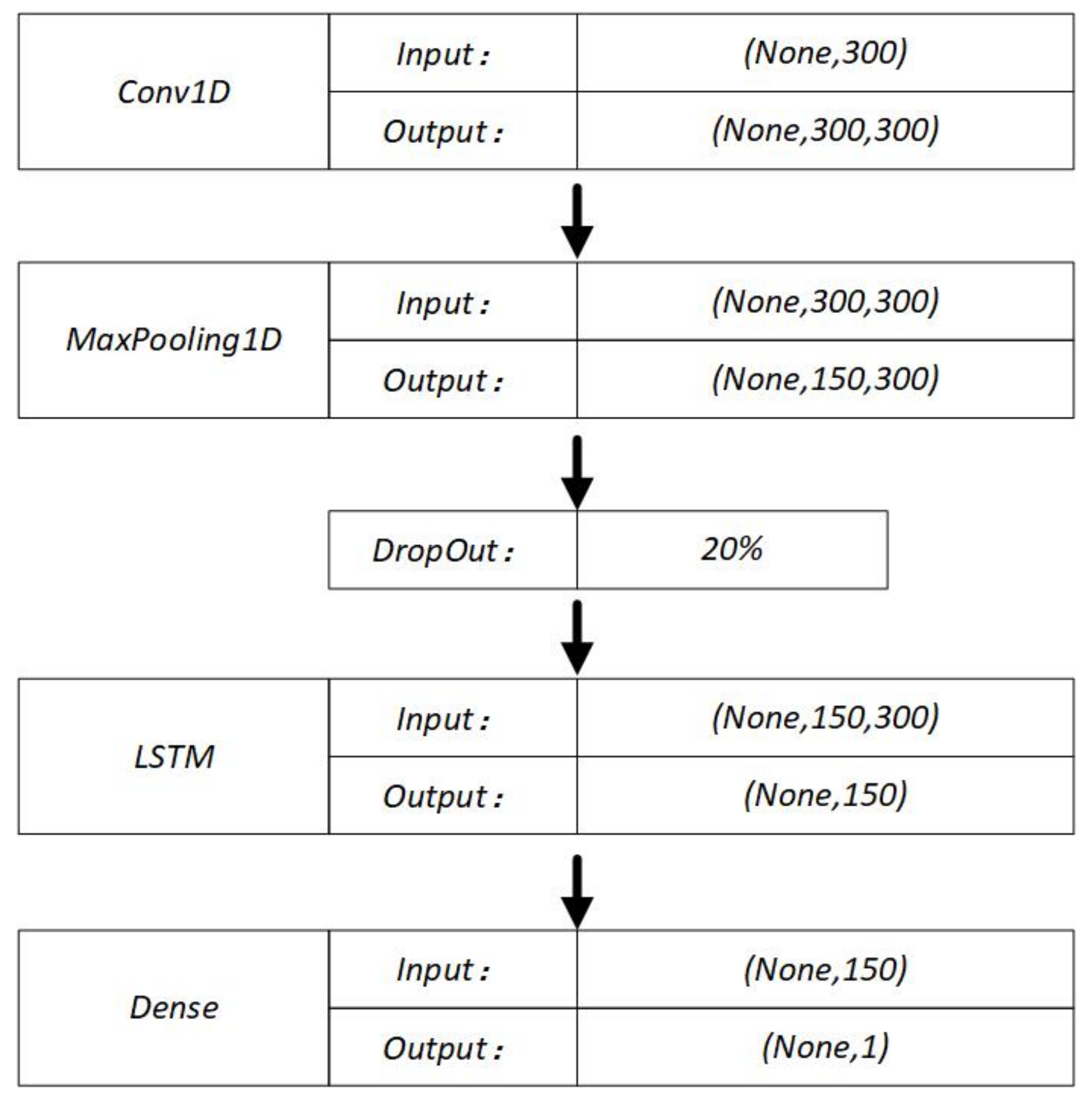
Building upon the ConvLSTM model, Geng et al. proposed a composite architecture called LightNet, which integrates the WRF model [41]. The LightNet structure is divided into four components: the WRF encoder, the observation encoder, the fusion module, and the prediction decoder, shown in

Table 1. LightNet architecture [41]. Used with permission of ResearchGate from Geng, Y.A.; Li, Q.; Lin, T.; Jiang, L.; Xu, L.; Zheng, D.; Yao,W.; Lyu,W.; Zhang, Y. Lightnet: A dual spatiotemporal encoder network model for lightning prediction. In Proceedings of the 25th ACM SIGKDD International Conference on Knowledge Discovery and Data Mining, Anchorage, AK, USA, 4–8 August 2019; pp. 2439–2447, 2019, permission conveyed through Copyright Clearance Center, Inc.

Module	Notation	Size	Stride
WRF Encoder	$Con{v}_1$	[7 × 7, 64]	2
	ConvLSTM	[5 × 5, 128]	1
Obs. Encoder	$Con{v}_2$	[7 × 7, 4]	2
	ConvLSTM	[5 × 5, 8]	1
Fusion Module	$Con{v}_3$	[1 × 1, 64]	1
	$Con{v}_4$	[1 × 1, 64]	1
Pred. Decoder	$Con{v}_5$	[7 × 7, 4]	2
	ConvLSTM	[5 × 5, 64]	1
	DeConv	[7 × 7, 64]	2
	$Con{v}_6$	[1 × 1, 1]	1

. The WRF encoder was primarily responsible for processing the simulation data produced by the WRF model. This data included various parameters, such as the cloud ice mixing ratio, snow mixing ratio, graupel mixing ratio, radar reflectivity, and the maximum vertical wind component. On the other hand, the observation encoder was designed to handle the processing of observational data. Both encoders adopted the same approach, going through a convolutional layer and inputting the convolution results into the ConvLSTM network to obtain two tensors, $C^{wrf}$, $H^{wrf}$ and $C^{obs}$, $H^{obs}$. The fusion module applied a convolution operation to the WRF data and observation data, respectively, resulting in the final initialized input tensors $C^{fuse}$ and $H^{fuse}$. The prediction decoder acquired the fused features and made predictions. All variables were initialized as $C^{fuse}$ and $H^{fuse}$, as well as the input ${Conv}_5\left(L_{-1}\right)$. The input and output at time t > 0 are:

$$X_t={Conv}_5\left({\widehat{L}}_{t-1}\right)$$

(25)

$${\widehat{L}}_t=softmax\left({Conv}_6\left(DeConv\left(Y_t\right)\right)\right)$$

(26)

where ${\widehat{L}}_t$ is the final result. The perfomance of LightNet and its variants on different datasets, especially for six-hour prediction, is better than other methods. If combined with neighboring nodes, POD can reach up to 0.680, with values of FAR of 0.413 and ETS of 0.449. On the contrary, values of POD of 0.465, FAR of 0.733, and ETS of 0.194 were attained.

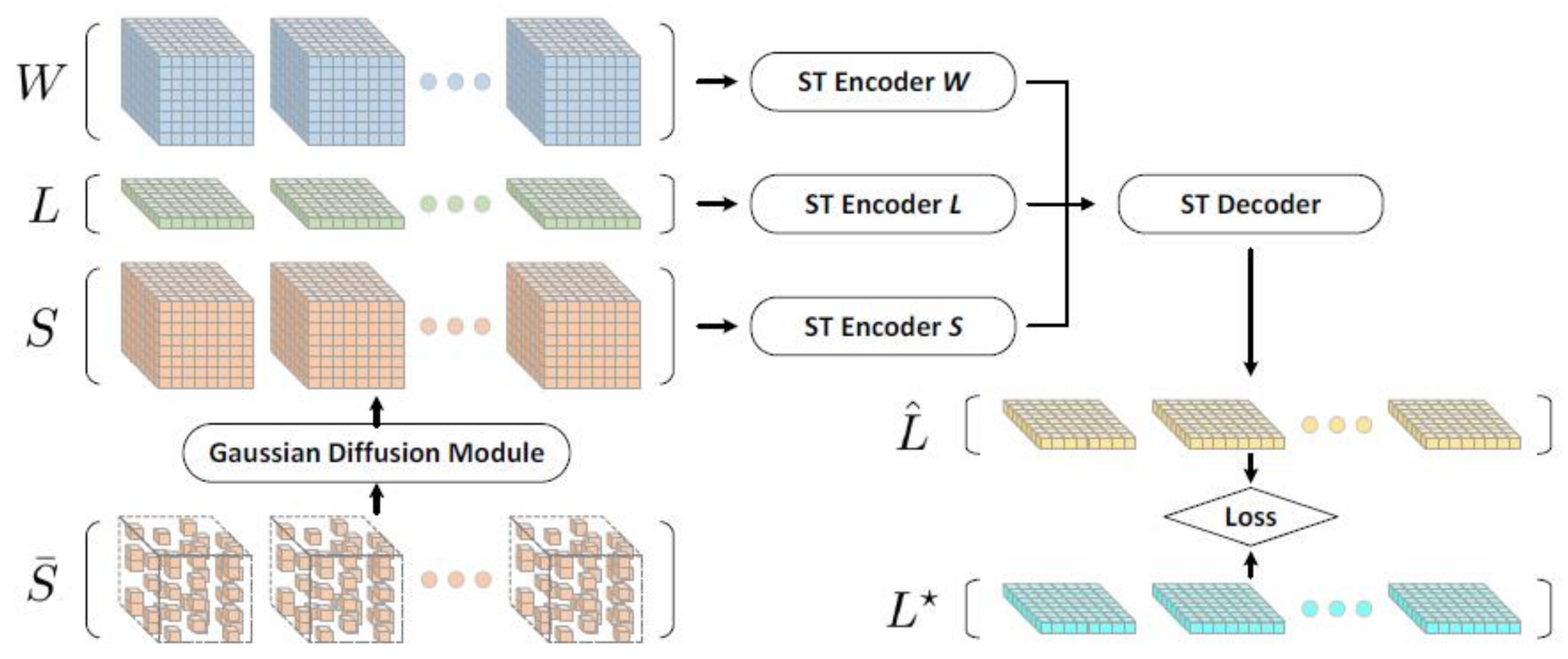
Geng et al. introduced a heterogeneous spatio-temporal network (HSTN) for lightning prediction, aimed at extracting knowledge from multiple heterogeneous spatio-temporal data sources [42]. The HSTN consists of three modules: the Gaussian diffusion module, the spatio-temporal encoder, and the spatio-temporal decoder. The Gaussian diffusion module converted the sparse tensor $\overline{S}$ into a dense form S (the weather station observation data, real four-dimensional data). The Gaussian diffusion module, founded upon the principles of Gaussian distribution, underwent a series of mathematical transformations and derivations to yield the resultant dense tensor. Three spatio-temporal encoders extracted information from W (the WRF simulation data, real four-dimensional data), L (the lightning observation data, binary three-dimensional data) and S. The spatio-temporal encoder was built based on ConvLSTM through initializing all states of ConvLSTM as zero. The spatio-temporal decoder merged all information and produced lightning prediction. Meanwhile, multi-scale pooling loss was employed to address the shortsightedness issue caused by grid-wise losses. Multi-scale pooling involves applying maximum pooling separately to both the predicted results and the actual outcomes and employing weighted cross-entropy to balance the disparities between lightning and non-lightning grids. The architecture of HSTN is shown in Figure 6. The data source was a real lightning dataset’s observation parameters, collected from 237 weather stations in North China. The performance of a six-hour dataset combined with neighboring nodes was best, achieving values of POD up to 0.692, FAR of 0.404, and ETS of 0.459.

Essa et al. conducted a study on the predictive capability of an LSTM model in predicting short-term lightning flash density within South Africa [43]. The research focused on predicting lightning flash densities over intervals of one hour, three hours, and twenty-four hours. The architecture of their LSTM model comprised an initial layer with 50 units, followed by two layers, each containing 25 units, and a final dense layer employing a Leaky ReLU activation function. The model optimization was performed using the Adam optimizer, targeting the minimization of the MSE. MAE increased with longer forecast periods. The perfomance of different datasets corresponded to a POD and FAR ratio of 32% and 51% and a POD and FAR ratio of 27% and 79%.

5. Hybrid Neural Network Methods

Hybrid neural networks combine different types of neural networks, leveraging the strengths of each to better accommodate varying data types and task requirements, thereby enhancing the model’s performance. Given the complexity and variety of lightning observation data, employing hybrid neural network models for lightning prediction is a prevalent approach. The most common amalgamation involves coupling CNNs with RNNs or LSTM networks.

Guastavino et al. put forth a long-term recurrent convolutional network (LRCN) which fused CNN and LSTM networks to devise spatio-temporal deep learning models using radar data to predict lightning occurrences [44]. The CNN was employed to extract spatial features from the dataset. These features were subsequently broken down into sequential components and supplied to the LSTM network for analysis. Finally, the output from the LSTM layer was passed into the fully connected layer, where the sigmoid activation function was used to generate the probability distribution of the positive class. Results on the test set obtained by using the TSS (true skill statistic) ensemble and wTSS (weighted true skill statistic) ensemble strategies are shown in

Table 2. Results of [44].

Strategy	TSS	CSI	wFP	wFN	wTSS	wCSI
wTSS	0.78 (±0.04)	0.17 (±0.02)	243.88 (±41.34)	6.79 (±1.64)	0.68 (±0.04)	0.10 (±0.02)
TSS	0.77 (±0.05)	0.17 (±0.03)	240.99 (±60.57)	7.24 (±2.60)	0.67 (±0.06)	0.10 (±0.02)

.

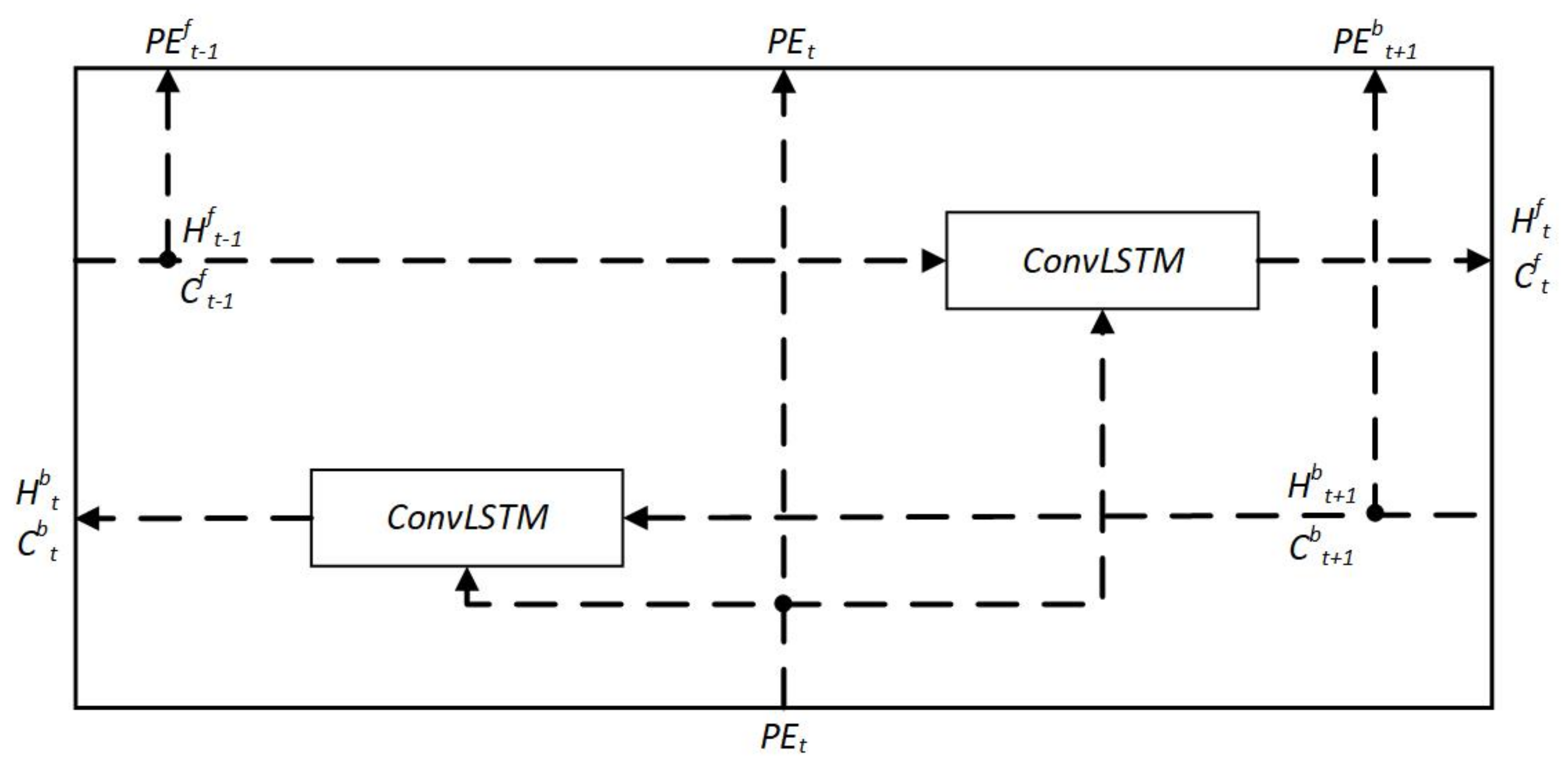
Zhou et al. extended upon LightNet, proposing LightNet+ [45]. This network represents a sophisticated hybrid neural network. It is composed of three modules: the SpatioTemporal (ST) encoder module for lightning observations, the bi-directional spatioTemporal (BDST) propagator module for WRF simulations, and the non-local spatio-temporal(NLST) module for lightning forecasts. The ST module initially employs a convolution layer to subsample the raw data, followed by a ConvLSTM model that extracts trend information from the compact lightning observation features. The BDST module is bifurcated into two components: a subsampling module and a dual ConvLSTM (DCLSTM). This module also uses a convolution layer for subsampling the WRF simulation data, followed by the DCLSTM to fully harness information both preceding and succeeding the t-th hour. The structure of the DCLSTM is illustrated in Figure 7. For the NLST module, a non-local fusion unit (NLFU) is introduced. The NLFU initially uses a convolution operation with a kernel size of 1 × 1 to extract features after amalgamating the historical lightning state trend, the past WRF trend information, and the future trend data into a comprehensive trend profile. This is followed by a two-stage attention mechanism to uncover informative long-range correlations. Finally, the data passes through the ConvLSTM module and a Deformable CNN, and it is subsampled using deconvolution (deConv) to produce the final output. Compared with several state-of-the-art data-driven lightning forecasting methods, LightNet+ yields the overall best performance with twelve-hour cumulative scores for TS of 0.211 and ETS of 0.193 and last-six-hour cumulative scores for TS of 0.125 and ETS of 0.116.

6. Discussion

Deep learning-based lightning prediction primarily focuses on directly analyzing observed parameters, often without the selection or filtering of these parameters. The accuracy of such models remains an area that warrants enhancement. This straightforward methodology could overlook intricate interrelationships among the observational parameters or the underlying physics driving lightning occurrences.

1. Parameter selection based on lightning mechanisms: Rather than indiscriminately using all observed parameters, a more discerning approach could involve parameter selection based on the underlying mechanisms of lightning formation. This would involve a deeper understanding of meteorology and the physics of atmospheric electricity, thereby ensuring that the most relevant and influential parameters are input into the model. Such a focused approach might eliminate noise and irrelevant information, potentially enhancing prediction accuracy.

2. Multimodal data fusion: Another promising avenue is the fusion of multimodal data. Instead of analyzing disparate data forms independently, combining various forms of data organically can provide a holistic view. By coalescing data from different sensors or observational platforms, deep learning networks can be exposed to a richer set of inputs, potentially enhancing their capacity to discern patterns and make accurate predictions.

3. Leveraging adjacent observational nodes: Incorporating data from neighboring observational nodes can enrich the contextual understanding of local atmospheric conditions. This spatial embedding ensures that the localized conditions leading to lightning formation are not viewed in isolation but are seen in the context of broader atmospheric dynamics. Integrating neighboring node data with the current node can offer a more comprehensive input for the network, potentially boosting predictive accuracy.

4. Expert-guided deep learning prediction: Lastly, instead of relying solely on algorithmic predictions, integrating expert knowledge from traditional lightning prediction methods can guide and refine deep learning-based forecasts. Such an interdisciplinary approach can combine the strengths of empirical knowledge and computational prowess. Furthermore, predictions can be provided with expert interpretations, lending more credibility and context to the forecasts.

In conclusion, while deep learning offers a promising toolset for lightning prediction, its integration with domain expertise, data fusion techniques, and a keen understanding of the intricacies of observational parameters can push the boundaries of prediction accuracy. Leveraging these strategies can pave the way for more reliable, insightful, and actionable lightning forecasts in the future.

7. Conclusions

From the above description, data-driven deep learning plays an important part in the field of lightning prediction. Evidently, deep learning methods, especially CNNs and RNNs, have demonstrated exceptional performance when dealing with complex multi-dimensional spatial and temporal data.

Traditional lightning prediction methods might rely on heuristic rules or simplified physical models, which might be inadequate to capture the full complexity of lightning formation. In contrast, CNNs and RNNs are capable of learning and extracting meaningful features from vast historical and real-time data, leading to more accurate predictions of lightning occurrences. This capability significantly surpasses the accuracy of conventional methods.

Furthermore, as more meteorological data become available and the resolution and quality of the data continually improve, deep learning methods will continue to be optimized and adapt to these new data sources. This implies that in the future, these advanced algorithms will provide earlier and more precise lightning alerts, thereby safeguarding lives and property.

In conclusion, data-driven deep learning, especially CNNs and RNNs, has not only made significant contributions to lightning prediction but also holds tremendous potential and prospects for future applications.

Table 3. Summary of lightning prediction methods.

Methods	Generalize	Specific Methods in Articles	Data Source
Numerical Prediction Methods	In accordance with the principles of lightning genesis, relevant observation parameters are used to calculate the lightning potential index (LPI) and positive ratio (PR), determining the probability of lightning occurrence.	LPI [7]	Total mass flux of liquid water and ice
		PR92 [8]	The intensity of updrafts and the intensity of updrafts
		PR93 [9]	Radiosonde data
		PR94 [10]	Global convective cloud data
		Grid LPI [11]	Total mass flux of liquid water and ice from 1 to 4 km
		POT + LPI [12]	Total mass flux of liquid water and ice
Traditional Machine Learning Methods	Employing manual calculations, key lightning data features are hand-extracted, and then traditional machine learning methods such as support vector machines (SVM) and simple artificial neural networks (simple ANN) are utilized based on the extracted features for classification.	EEMD + SVM/ANN [18]	Observation meteorological parameters
		Gradient boosting machine learning [21]	Binary meteosat satellite images and lightning detected data
		Undersampling + shallow neural network/DT [22]	Observation meteorological parameters
		Back-propagation neural network [23]	Observation meteorological parameters
		Undersampling + SVM/RF [24]	Observation meteorological parameters
Convolutional Neural Network Methods	Integrating image data such as satellite images, electromagnetic and acoustic signals, or converting lightning data into image form allows the utilization of convolution to extract features and conduct predictions.	U-Net + ResNet-v2 [26]	Geostationary satellite images
		KL + CNN + MLP [29]	Time-series observation meteorological parameters
		Spectrograms + CNN [31]	Random noise, lightning sounds, and background noise
		Sliding window + CNN [32]	3D weather radar data
Recurrent Neural Network Methods	The most commonly used deep learning method for lightning prediction primarily processes sequential data, often combining with existing methodologies in a variant form to achieve more accurate predictions.	OK + LSTM [37]	Time-series electric field data
		Convolution + LSTM [39]	Time-series electric field data
		ConvLSTM [40]	Spatio-temporal data
		LightNet (WRF + ConvLSTM) [41]	Spatio-temporal WRF simulation data
		HSTN (Gaussian diffusion + WRF + CNN + ConvLSTM) [42]	The weather station observation data, real four-dimensional data, the WRF simulation data and binary three-dimensional data
		LSTM [43]	Lightning flash density
Hybrid Neural Network Methods	Combining multiple neural network models often involves the use of one network model for feature extraction and another for prediction. With more information contained in the features, this approach aids in improving the accuracy of predictions.	LRCN (CNN + LSTM) [44]	Radar data
		CNN + ConvLSTM + Dual ConvLSTM (DCLSTM) + Deformable CNN + deConv [45]	WRF simulation data

provides a summary of the lightning prediction methods outlined in this article.