
Climate Change Effects through MFDFA Study of Temperature in Serbia

 , , , and
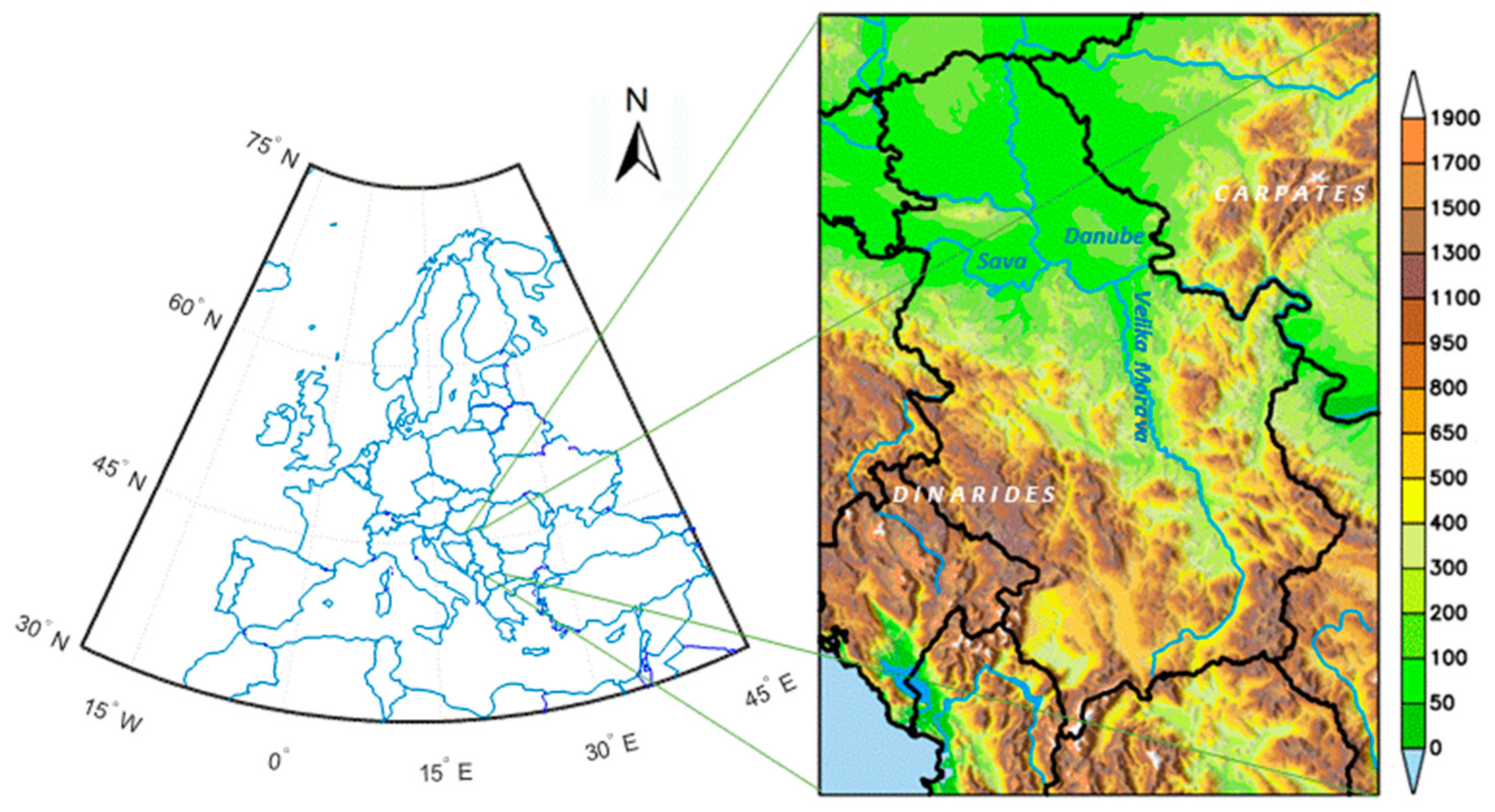
Abstract
:1. Introduction
2. Data and Methodology
2.1. Study Area and Dataset
2.2. Multifractal Detrended Fluctuation Analysis
3. Results and Discussion
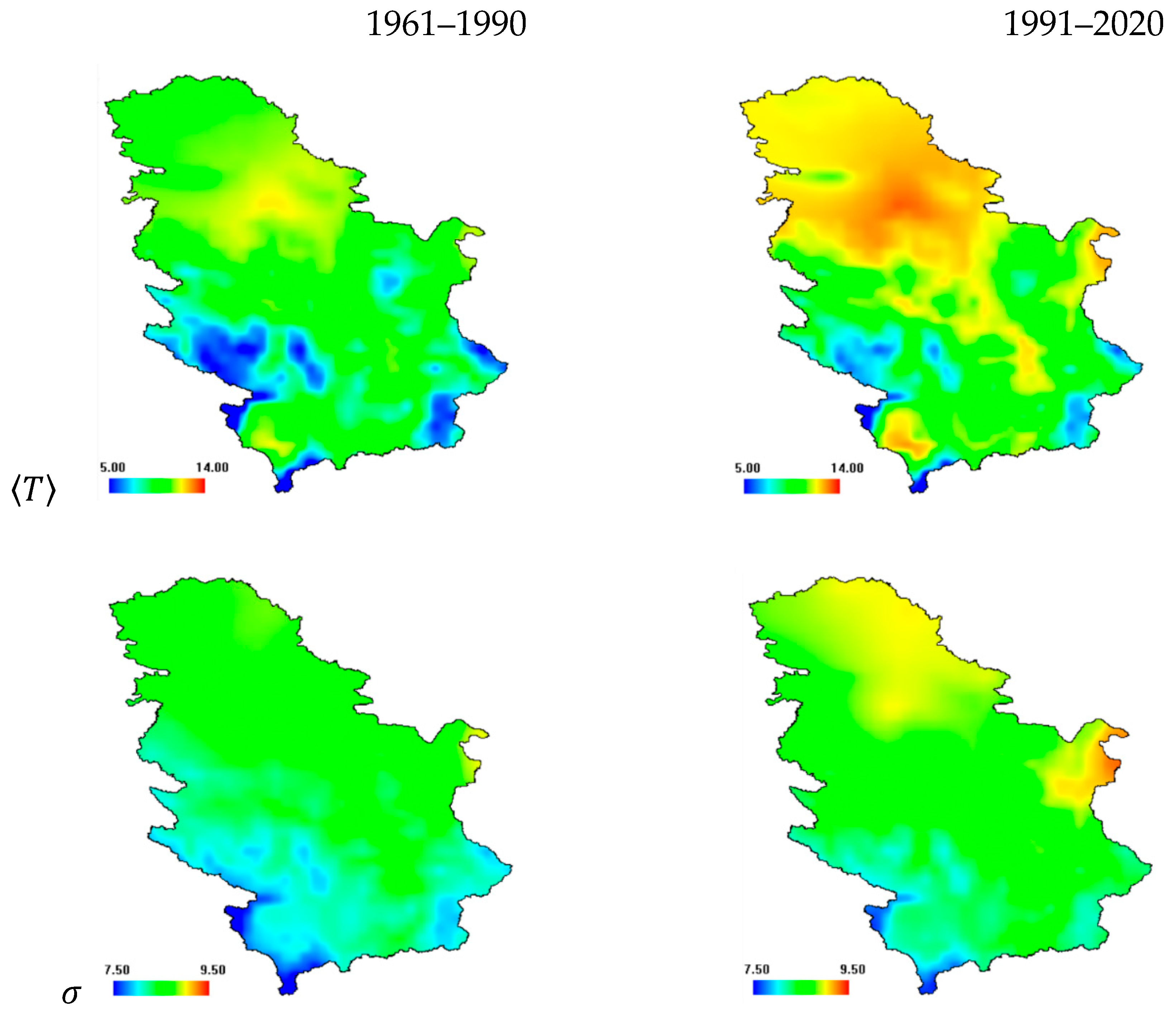
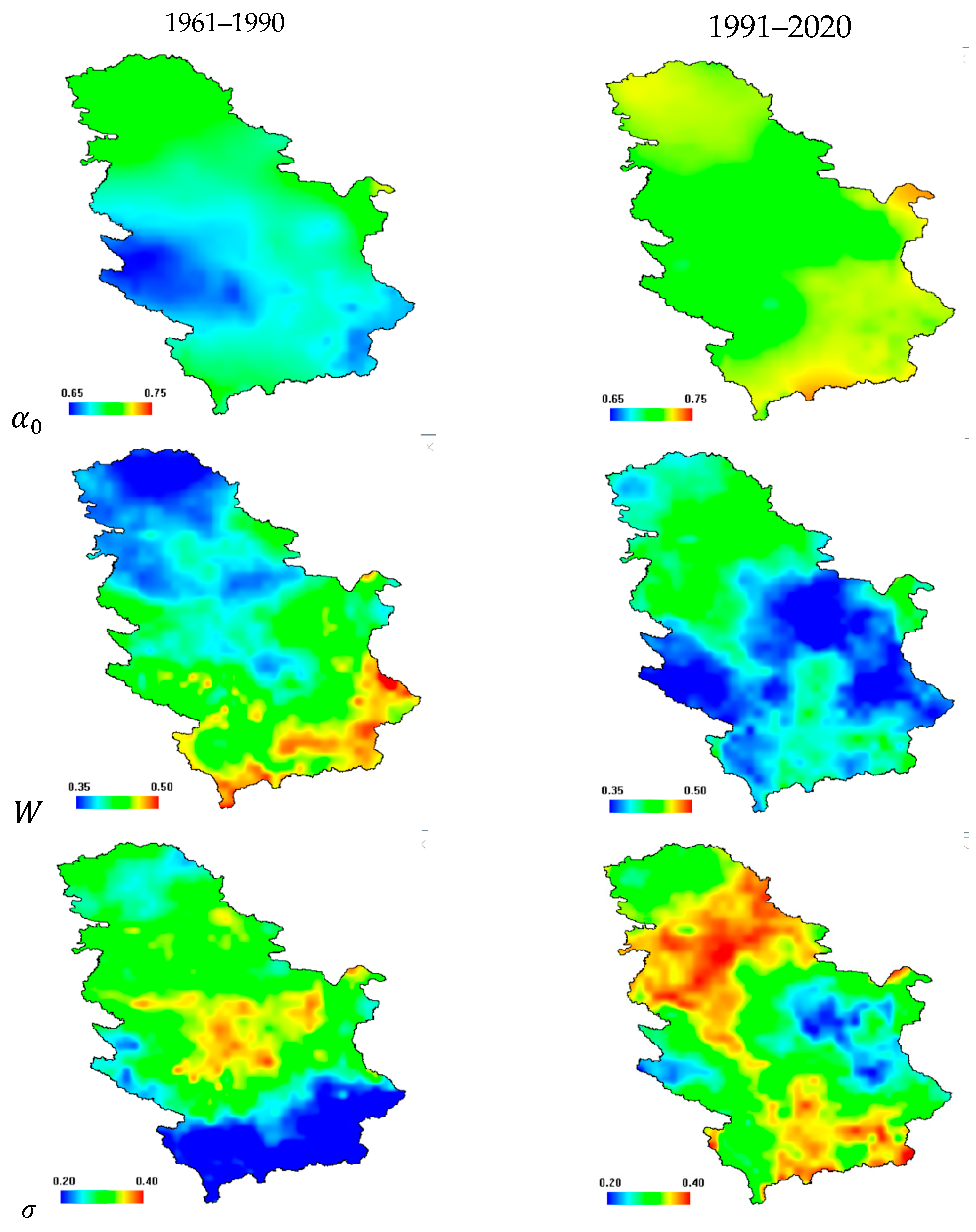
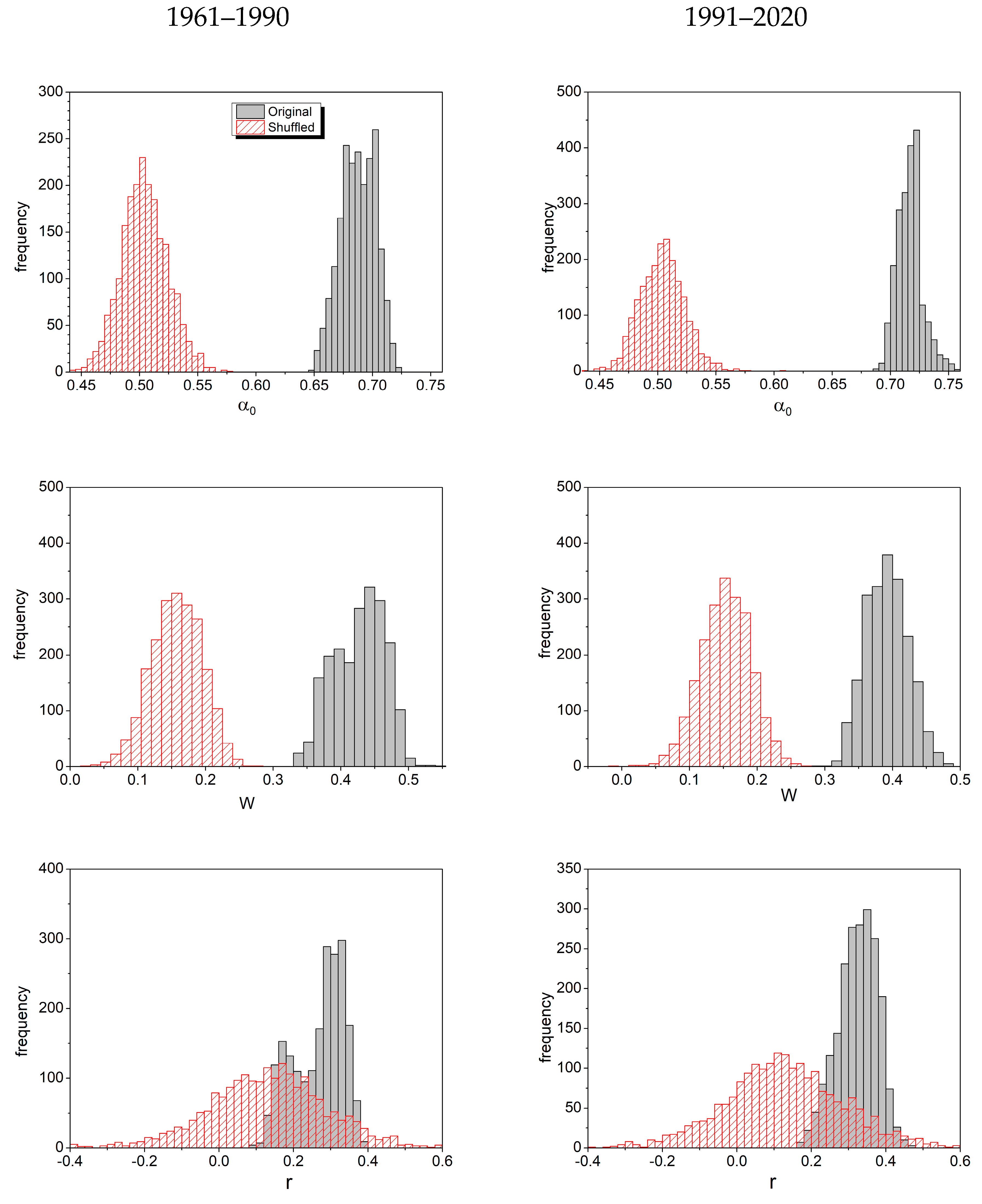
3.1. Multifractal Analysis
3.2. Comparison with Studies from Other Countries
4. Conclusions
Author Contributions
Funding
Institutional Review Board Statement
Informed Consent Statement
Data Availability Statement
Acknowledgments
Conflicts of Interest
References
- Rind, D. Complexity and climate. Science 1999, 284, 105–107. [Google Scholar] [CrossRef]
- Rodriguez-Iturbe, I.; Febres De Power, B.; Sharifi, M.B.; Georgakakos, K.P. Chaos in rainfall. Water Resour. 1989, 25, 1667–1675. [Google Scholar] [CrossRef]
- Fuwape, I.A.; Ogunjo, S.T.; Oluyamo, S.S.; Rabiu, A.B. Spatial variation of deterministic chaos in mean daily temperature and rainfall over Nigeria. Theor. Appl. Climatol. 2017, 130, 119–132. [Google Scholar] [CrossRef]
- Chang, T.P.; Ko, H.H.; Liu, F.J.; Chen, P.H.; Chang, Y.P.; Liang, Y.H.; Jang, H.Y.; Lin, T.C.; Chen, Y.H. Fractal dimension of wind speed time series. Appl. Energy 2012, 93, 742–749. [Google Scholar] [CrossRef]
- Lovejoy, S.; Mandelbrot, B.B. Fractal properties of rain, and a fractal model. Tellus A 1985, 37, 209–232. [Google Scholar] [CrossRef]
- Mali, P. Multifractal characterization of global temperature anomalies. Theor. Appl. Climatol. 2015, 121, 641–648. [Google Scholar] [CrossRef]
- Kavasseri, R.G.; Nagarajan, R. A multifractal description of wind speed records. Chaos Solitons Fractals 2005, 24, 165–173. [Google Scholar] [CrossRef]
- Kantelhardt, J.W.; Koscielny-Bunde, E.; Rybski, D.; Braun, P.; Bunde, A.; Havlin, S. Long-term persistence and multifractality of precipitation and river runoff records. J. Geophys. Res. 2006, 111, 1–13. [Google Scholar] [CrossRef]
- Li, Q.; Zuntao, F. Permutation entropy and statistical complexity quantifier of nonstationarity effect in the vertical velocity records. Phys. Rev. E Stat. Nonlinear Soft Matter Phys. 2014, 89, 012905. [Google Scholar] [CrossRef]
- Silva, A.S.A.D.; Barreto, I.D.D.C.; Cunha-Filho, M.; Menezes, R.S.C.; Stosic, B.; Stosic, T. Multiscale complexity analysis of rainfall in northeast Brazil. Water 2021, 13, 3213. [Google Scholar] [CrossRef]
- Tongal, H.; Sivakumar, B. Transfer entropy coupled directed–weighted complex network analysis of rainfall dynamics. Stoch. Environ. Res. Risk Assess. 2022, 36, 851–867. [Google Scholar] [CrossRef]
- Donges, J.F.; Zou, Y.; Marwan, N.; Kurths, J. Complex networks in climate dynamics: Comparing linear and nonlinear network construction methods. Eur. Phys. J. Spec. Top. 2009, 174, 157–179. [Google Scholar] [CrossRef]
- Onyutha, C.; Rutkowska, A.; Nyeko-Ogiramoi, P.; Willems, P. How well do climate models reproduce variability in observed rainfall? A case study of the Lake Victoria basin considering CMIP3, CMIP5 and CORDEX simulations. Stoch. Environ. Res. Risk Assess. 2019, 33, 687–707. [Google Scholar] [CrossRef]
- García-Marín, A.P.; Jiménez-Hornero, F.J.; Ayuso-Muñoz, J.L. Multifractal analysis as a tool for validating a rainfall model. Hydrol. Process. 2008, 22, 2672–2688. [Google Scholar] [CrossRef]
- Deepthi, B.; Sivakumar, B. General circulation models for rainfall simulations: Performance assessment using complex networks. Atmos. Res. 2022, 278, 106333. [Google Scholar] [CrossRef]
- Lovejoy, S.; Schertzer, D. The Weather and Climate: Emergent Laws and Multifractal Cascades, 2nd ed.; Cambridge University Press: Cambridge, UK, 2018; 480p. [Google Scholar]
- Jiang, L.; Zhang, J.; Liu, X.; Li, F. Multi-fractal scaling comparison of the air temperature and the surface temperature over China. Phys. A Stat. Mech. Appl. 2016, 462, 783–792. [Google Scholar] [CrossRef]
- Da Silva, H.S.; Silva, J.R.S.; Stosic, T. Multifractal analysis of air temperature in Brazil. Phys. A Stat. Mech. Appl. 2020, 549, 124333. [Google Scholar] [CrossRef]
- Akinsusi, J.; Ogunjo, S.; Fuwape, I. Nonlinear dynamics and multifractal analysis of minimum–maximum temperature and solar radiation over Lagos State, Nigeria. Acta Geophys. 2022, 70, 2171–2178. [Google Scholar] [CrossRef]
- Adarsh, S.; Nourani, V.; Archana, D.S.; Dharan, D.S. Multifractal description of daily rainfall fields over India. J. Hydrol. 2020, 586, 124913. [Google Scholar] [CrossRef]
- Gómez-Gómez, J.; Carmona-Cabezas, R.; Sánchez-López, E.; de Ravé, E.G.; Jiménez-Hornero, F.J. Multifractal fluctuations of the precipitation in Spain (1960–2019). Chaos Solitons Fractals 2022, 157, 111909. [Google Scholar] [CrossRef]
- De Lima, M.I.P.; Grasman, J. Multifractal analysis of 15-min and daily rainfall from a semi-arid region in Portugal. J. Hydrol. 1999, 220, 1–11. [Google Scholar] [CrossRef]
- Tan, X.; Gan, T.Y. Multifractality of Canadian precipitation and streamflow. Int. J. Climatol. 2017, 37, 1221–1236. [Google Scholar] [CrossRef]
- Liu, Z.; Xu, J.; Chen, Z.; Nie, Q.; Wei, C. Multifractal and long memory of humidity process in the Tarim River Basin. Stoch. Environ. Res. Risk Assess. 2014, 28, 1383–1400. [Google Scholar] [CrossRef]
- Garcia-Marin, A.P.; Estévez, J.; Jiménez-Hornero, F.J.; Ayuso-Muñoz, J.L. Multifractal analysis of validated wind speed time series. Chaos 2013, 23, 013133. [Google Scholar] [CrossRef] [PubMed]
- Laib, M.; Golay, J.; Telesca, L.; Kanevski, M. Multifractal analysis of the time series of daily means of wind speed in complex regions. Chaos Solitons Fractals 2018, 109, 118–127. [Google Scholar] [CrossRef]
- Dos Santos, F.S.; do Nascimento, K.K.F.; da Silva Jale, J.; Stosic, T.; Marinho, M.H.; Ferreira, T.A. Mixture distribution and multifractal analysis applied to wind speed in the Brazilian Northeast region. Chaos Solitons Fractals 2021, 144, 110651. [Google Scholar] [CrossRef]
- Zeng, Z.; Yang, H.; Zhao, R.; Meng, J. Nonlinear characteristics of observed solar radiation data. Sol. Energy 2013, 87, 204–218. [Google Scholar] [CrossRef]
- Dos Santos, F.S.; Do Nascimento, K.K.F.; Jale, J.S.; Xavier Júnior, S.F.A.; Ferreira, T.A. Multifractal Analysis of Solar Radiation in the Northeastern Region of Brazil. Fractals 2023, 31, 2350025. [Google Scholar] [CrossRef]
- Maruyama, F. The relation among the solar activity, the total ozone, QBO, NAO, and ENSO by wavelet-based multifractal analysis. J. Appl. Math. Phys. 2018, 6, 1301–1314. [Google Scholar] [CrossRef]
- Varotsos, C.A.; Cracknell, A.P.; Efstathiou, M.N. The global signature of the el Niño/La Niña southern oscillation. Int. J. Remote Sens. 2018, 39, 5965–5977. [Google Scholar] [CrossRef]
- Folland, C.K.; Karl, T.R.; Christy, J.R.; Clarke, R.A.; Gruza, G.V.; Jouzel, J.; Mann, M.E.; Oerlemans, J.; Salinger, M.J.; Wang, S.W. Observed climate variability and change. In Climate Change 2001; Cambridge University Press: New York, NY, USA, 2001; pp. 99–181. [Google Scholar]
- Manabe, S. Role of greenhouse gas in climate change. Tellus A 2019, 71, 1620078. [Google Scholar] [CrossRef]
- Mikhaylov, A.; Moiseev, N.; Aleshin, K.; Burkhardt, T. Global climate change and greenhouse effect. Entrep. Sustain. Issues 2020, 7, 2897–2913. [Google Scholar] [CrossRef] [PubMed]
- Kantelhardt, J.W.; Zschiegner, S.A.; Koscielny-Bunde, E.; Havlin, S.; Bunde, A.; Stanley, H.E. Multifractal detrended fluctuation analysis of nonstationary time series. Phys. A Stat. Mech. Appl. 2002, 316, 87–114. [Google Scholar] [CrossRef]
- Bajat, B.; Blagojević, D.; Kilibarda, M.; Luković, J.; Tošić, I. Spatial analysis of the temperature trends in Serbia during the period 1961–2010. Theor. Appl. Climatol. 2015, 121, 289–301. [Google Scholar] [CrossRef]
- Ruml, M.; Gregorić, E.; Vujadinović, M.; Radovanović, S.; Matović, G.; Vuković, A.; Počuča, V.; Stojičić, D. Observed changes of temperature extremes in Serbia over the period 1961−2010. Atmos. Res. 2017, 183, 26–41. [Google Scholar] [CrossRef]
- Malinović-Milićcević, S.; Radovanović, M.M.; Stanojević, G.; Milovanović, B. Recent changes in Serbian climate extreme indices from 1961 to 2010. Theor. Appl. Climatol. 2016, 124, 1089–1098. [Google Scholar] [CrossRef]
- Unkašević, M.; Tošić, I. Trends in temperature indices over Serbia: Relationships to large-scale circulation patterns. Int. J Climatol. 2013, 33, 3152–3161. [Google Scholar] [CrossRef]
- Tošić, I.; Tošić, M.; Lazić, I.; Aleksandrov, N.; Putniković, S.; Djurdjević, V. Spatio-temporal changes in the mean and extreme temperature indices for Serbia. Int. J Climatol. 2023, 43, 2391–2410. [Google Scholar] [CrossRef]
- Unkašević, M.; Tošić, I. Seasonal analysis of cold and heat waves in Serbia during the period 1949–2012. Theor. Appl. Climatol. 2015, 120, 29–40. [Google Scholar] [CrossRef]
- Milovanović, B.; Schubert, S.; Radovanović, M.; Vakanjac, V.R.; Schneider, C. Projected changes in air temperature, precipitation and aridity in Serbia in the 21st century. Int. J Climatol. 2022, 42, 1985–2003. [Google Scholar] [CrossRef]
- Cornes, R.; van der Schrier, G.; van den Besselaar, E.J.M.; Jones, P.D. An Ensemble Version of the E-OBS Temperature and Precipitation Datasets. J. Geophys. Res. Atmos. 2018, 123, 9391–9409. [Google Scholar] [CrossRef]
- Muzy, J.F.; Bacry, E.; Arneodo, A. Wavelets and multifractal formalism for singular signals: Application to turbulence data. Phys. Rev. Lett. 1991, 67, 3515–3518. [Google Scholar] [CrossRef]
- Gu, G.-F.; Zhou, W.-X. Detrending moving average algorithm for multifractals. Phys. Rev. E 2010, 82, 011136. [Google Scholar] [CrossRef]
- Oswiecimka, P.; Kwapien, J.; Drozd, S. Wavelet versus detrended fluctuation analysis of multifractal structures. Phys. Rev. E 2006, 74, 016103. [Google Scholar] [CrossRef] [PubMed]
- Maity, A.K.; Pratihar, R.; Mitra, A.; Dey, S.; Agrawal, V.; Sanyal, S.; Banerjee, A.; Sengupta, R.; Ghosh, D. Multifractal detrended fluctuation analysis of alpha and theta EEG rhythms with musical stimuli. Chaos Solitons Fractals 2015, 81, 52–67. [Google Scholar] [CrossRef]
- Aggarwal, S.K.; Lovallo, M.; Khan, P.K.; Rastogi, B.K.; Telesca, L. Multifractal detrended fluctuation analysis of magnitude series of seismicity of Kachchh region, Western India. Phys. A Stat. Mech. Appl. 2015, 426, 56–62. [Google Scholar] [CrossRef]
- Balkissoon, S.; Fox, N.; Lupo, A. Fractal characteristics of tall tower wind speeds in Missouri. Renew. Energy 2020, 154, 1346–1356. [Google Scholar] [CrossRef]
- Wu, Y.; He, Y.; Wu, M.; Lu, C.; Gao, S.; Xu, Y. Multifractality and cross-correlation analysis of streamflow and sediment fluctuation at the apex of the Pearl River Delta. Sci. Rep. 2018, 8, 16553. [Google Scholar] [CrossRef]
- Wątorek, M.; Drożdż, S.; Kwapień, J.; Minati, L.; Oświęcimka, P.; Stanuszek, M. Multiscale characteristics of the emerging global cryptocurrency market. Phys. Rep. 2021, 901, 1–82. [Google Scholar] [CrossRef]
- Hurst, H. Long-term storage capacity of tanks. In Proceedings of the American Society of Civil Engineers; American Society of Civil Engineers: Reston, VA, USA, 1951; Volume 116, pp. 770–799. [Google Scholar]
- Mandelbrot, B.B. Fractal Geometry of Nature; Times Book: New York, NY, USA, 1982; 480p. [Google Scholar]
- Shimizu, Y.U.; Thurner, S.; Ehrenberger, K. Multifractal spectra as a measure of complexity in human posture. Fractals 2002, 10, 103–116. [Google Scholar] [CrossRef]
- Stosic, T.; Nejad, S.A.; Stosic, B. Multifractal analysis of Brazilian agricultural market. Fractals 2020, 28, 2050076. [Google Scholar] [CrossRef]
- Putniković, S.; Tošić, I.; Đurđević, V. Circulation weather types and their influence on precipitation in Serbia. Meteor. Atmos. Phys. 2016, 128, 649–662. [Google Scholar] [CrossRef]
- Mimić, G.; Mihailović, D.T.; Kapor, D. Complexity analysis of the air temperature and the precipitation time series in Serbia. Theor. Appl. Climatol. 2017, 127, 891–898. [Google Scholar] [CrossRef]
- Gómez-Gómez, J.; Carmona-Cabezas, R.; Ariza-Villaverde, A.B.; de Ravé, E.G.; Jiménez-Hornero, F.J. Multifractal detrended fluctuation analysis of temperature in Spain (1960–2019). Phys. A Stat. Mech. Appl. 2021, 578, 126118. [Google Scholar] [CrossRef]
- Burgueño, A.; Lana, X.; Serra, C.; Martínez, M.D. Daily extreme temperature multifractals in Catalonia (NE Spain). Phys. Lett. A 2014, 378, 874–885. [Google Scholar] [CrossRef]
- Kalamaras, N.; Tzanis, C.G.; Deligiorgi, D.; Philippopoulos, K.; Koutsogiannis, I. Distribution of Air Temperature Multifractal Characteristics Over Greece. Atmosphere 2019, 10, 45. [Google Scholar] [CrossRef]
- Philippopoulos, K.; Kalamaras, N.; Tzanis, C.G.; Deligiorgi, D.; Koutsogiannis, I. Multifractal detrended fluctuation analysis of temperature reanalysis data over Greece. Atmosphere 2019, 10, 336. [Google Scholar] [CrossRef]
- Baranowski, P.; Gos, M.; Krzyszczak, J.; Siwek, K.; Kieliszek, A.; Tkaczyk, P. Multifractality of meteorological time series for Poland on the base of MERRA-2 data. Chaos Solitons Fractals 2019, 127, 318–333. [Google Scholar] [CrossRef]
- Gos, M.; Baranowski, P.; Krzyszczak, J.; Kieliszek, A.; Siwek, K. Dynamics of meteorological time series on the base of ground measurements and retrospective data from MERRA-2 for Poland. Int. J. Climatol. 2021, 41, E1531–E1552. [Google Scholar] [CrossRef]
- Rahmani, F.; Fattahi, M.H. Climate change-induced influences on the nonlinear dynamic patterns of precipitation and temperatures (case study: Central England). Theor. Appl. Climatol. 2023, 152, 1147–1158. [Google Scholar] [CrossRef]


Disclaimer/Publisher’s Note: The statements, opinions and data contained in all publications are solely those of the individual author(s) and contributor(s) and not of MDPI and/or the editor(s). MDPI and/or the editor(s) disclaim responsibility for any injury to people or property resulting from any ideas, methods, instructions or products referred to in the content. |
© 2023 by the authors. Licensee MDPI, Basel, Switzerland. This article is an open access article distributed under the terms and conditions of the Creative Commons Attribution (CC BY) license (https://creativecommons.org/licenses/by/4.0/).
Share and Cite
Stosic, T.; Stosic, B.; Tošić, M.; Lazić, I.; Djurdjević, V.; Tošić, I. Climate Change Effects through MFDFA Study of Temperature in Serbia. Atmosphere 2023, 14, 1532. https://doi.org/10.3390/atmos14101532
Stosic T, Stosic B, Tošić M, Lazić I, Djurdjević V, Tošić I. Climate Change Effects through MFDFA Study of Temperature in Serbia. Atmosphere. 2023; 14(10):1532. https://doi.org/10.3390/atmos14101532
Chicago/Turabian StyleStosic, Tatijana, Borko Stosic, Milica Tošić, Irida Lazić, Vladimir Djurdjević, and Ivana Tošić. 2023. "Climate Change Effects through MFDFA Study of Temperature in Serbia" Atmosphere 14, no. 10: 1532. https://doi.org/10.3390/atmos14101532
APA StyleStosic, T., Stosic, B., Tošić, M., Lazić, I., Djurdjević, V., & Tošić, I. (2023). Climate Change Effects through MFDFA Study of Temperature in Serbia. Atmosphere, 14(10), 1532. https://doi.org/10.3390/atmos14101532