
Estimating Daily Temperatures over Andhra Pradesh, India, Using Artificial Neural Networks


Abstract
:1. Introduction
2. Data and Methodology
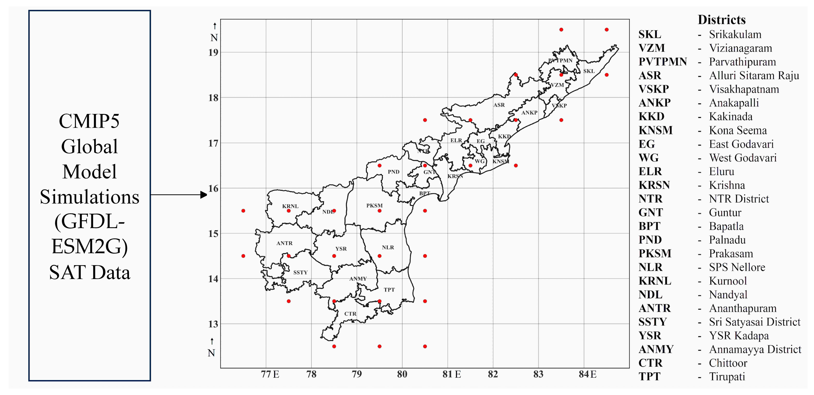
2.1. Data
2.2. Methodology
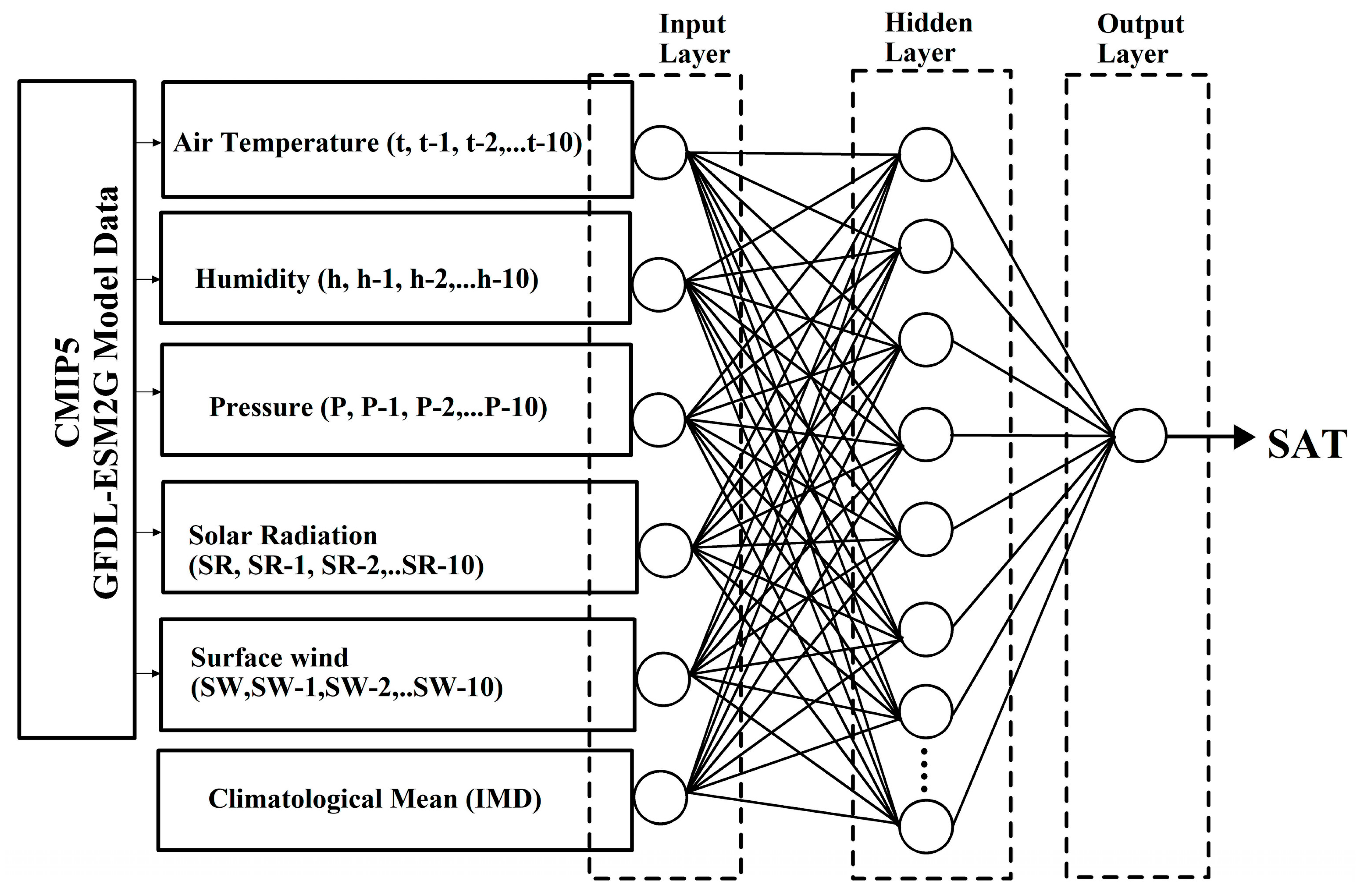
2.2.1. ANN Approach
2.2.2. Analysis
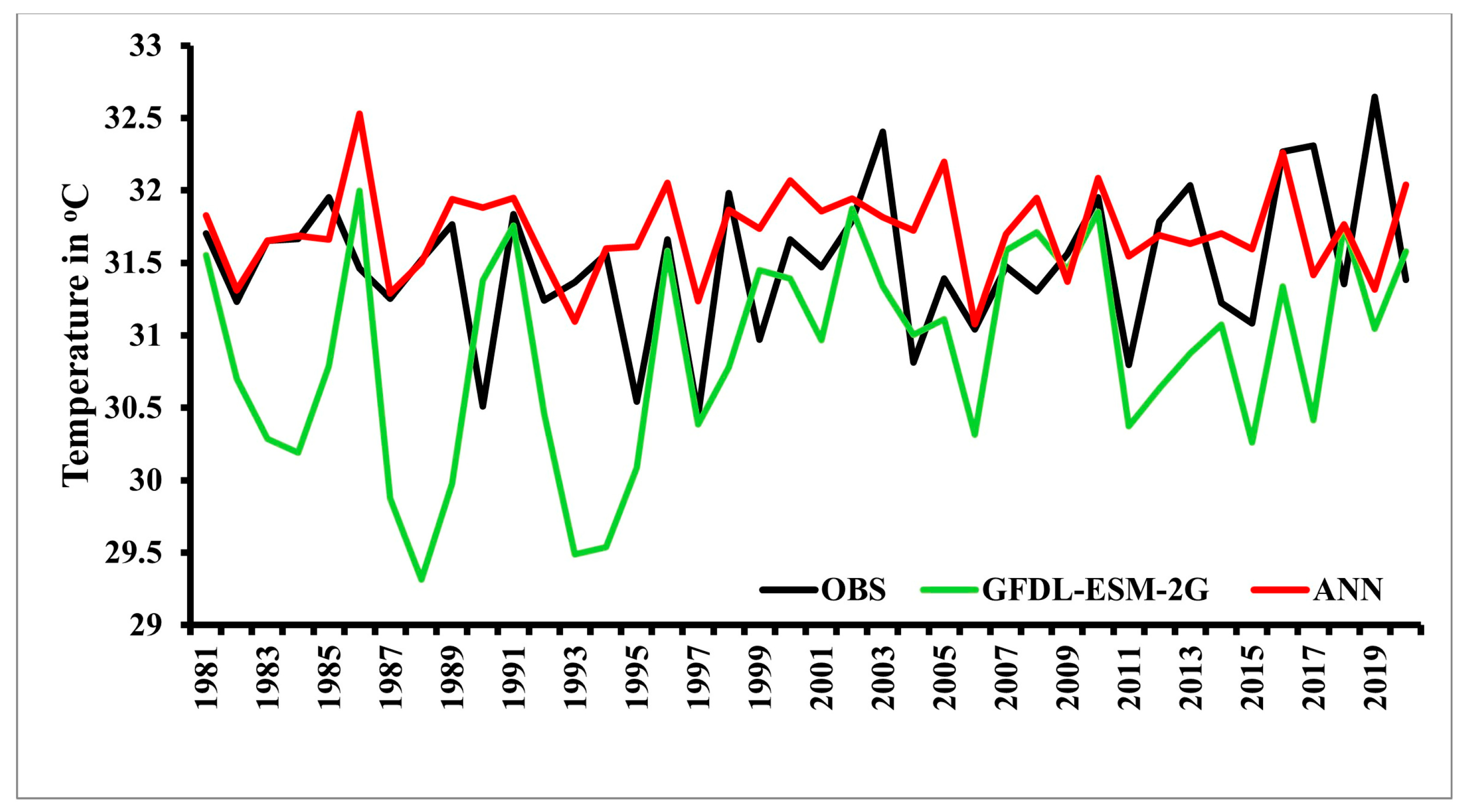
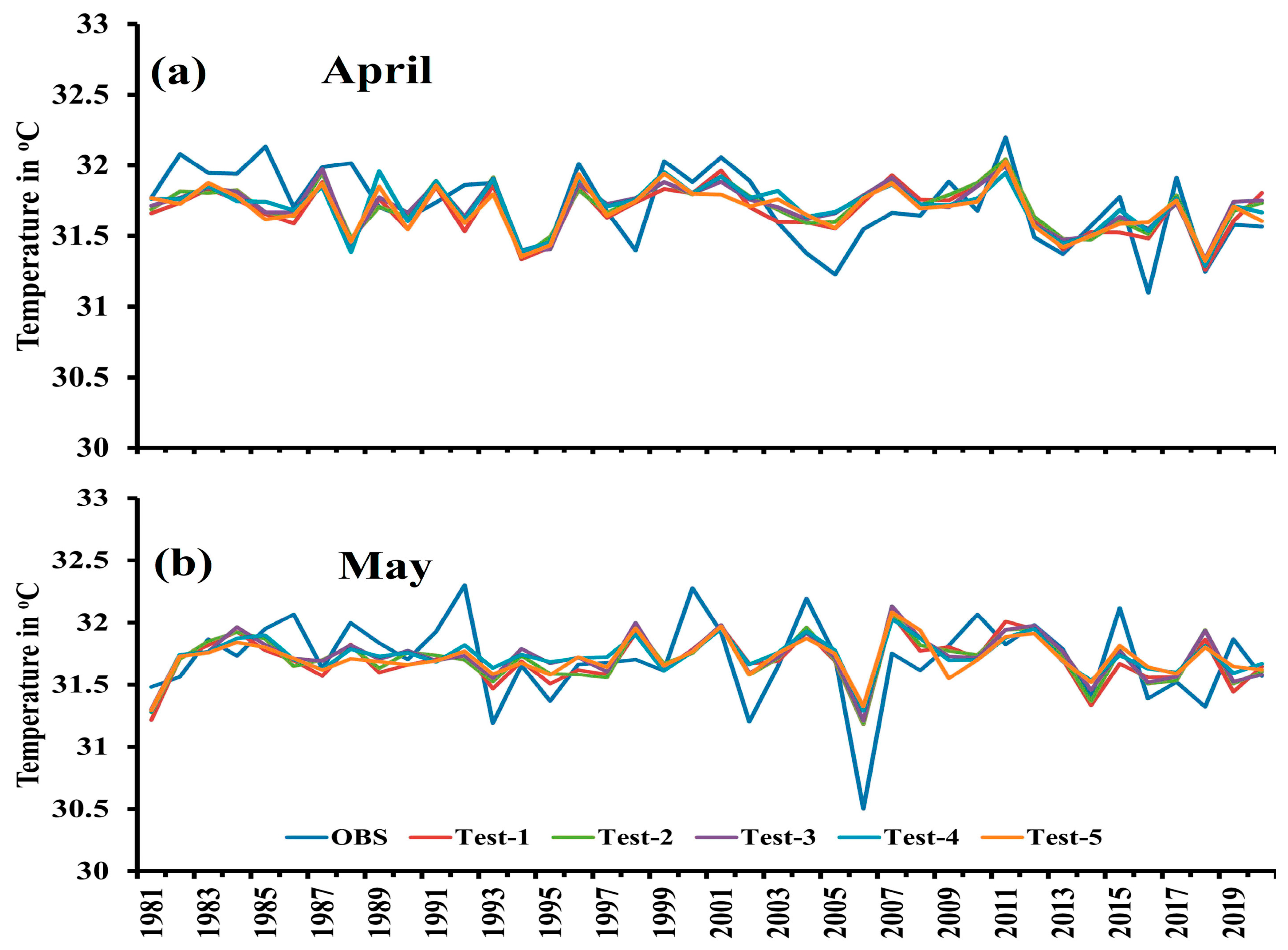
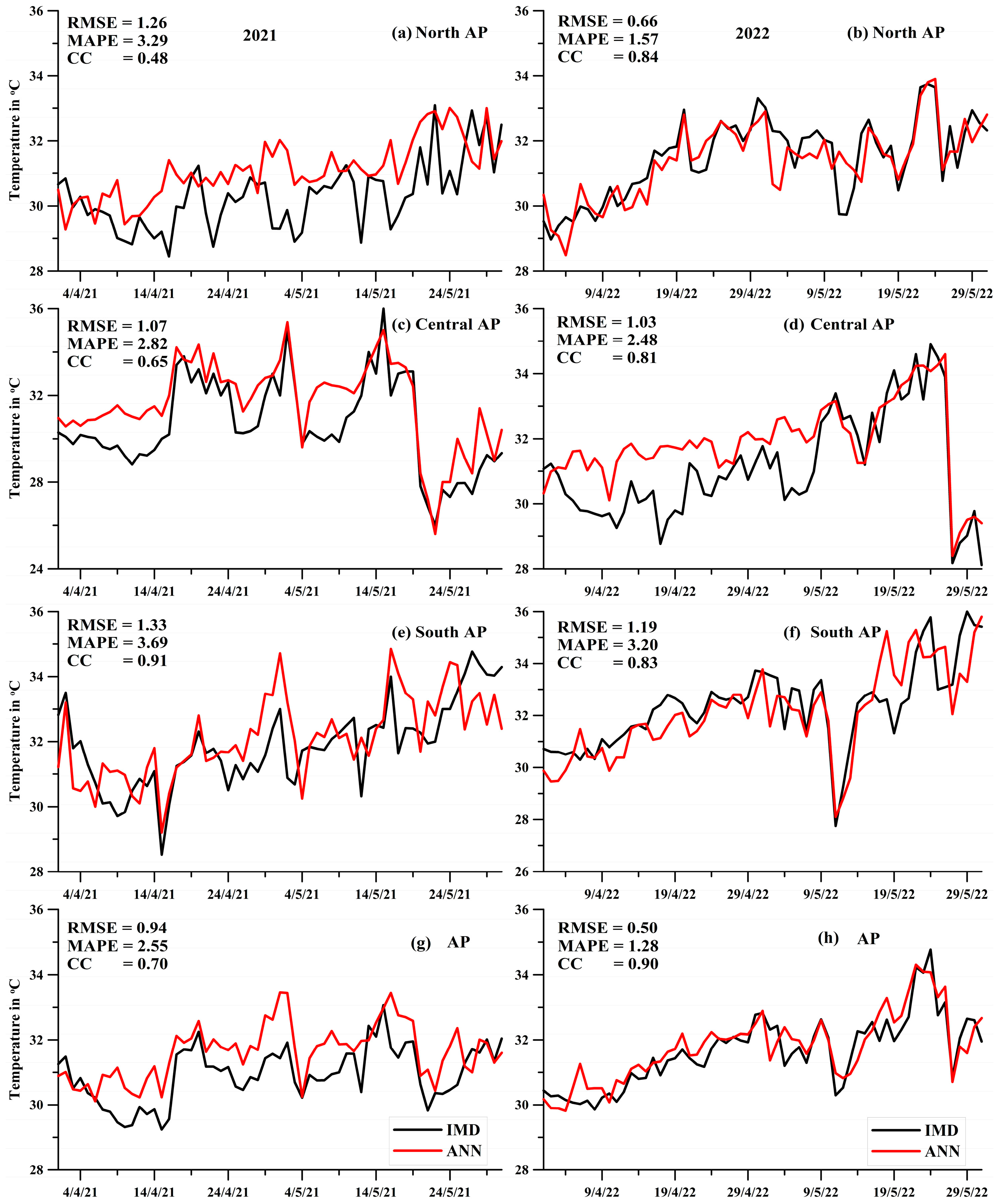
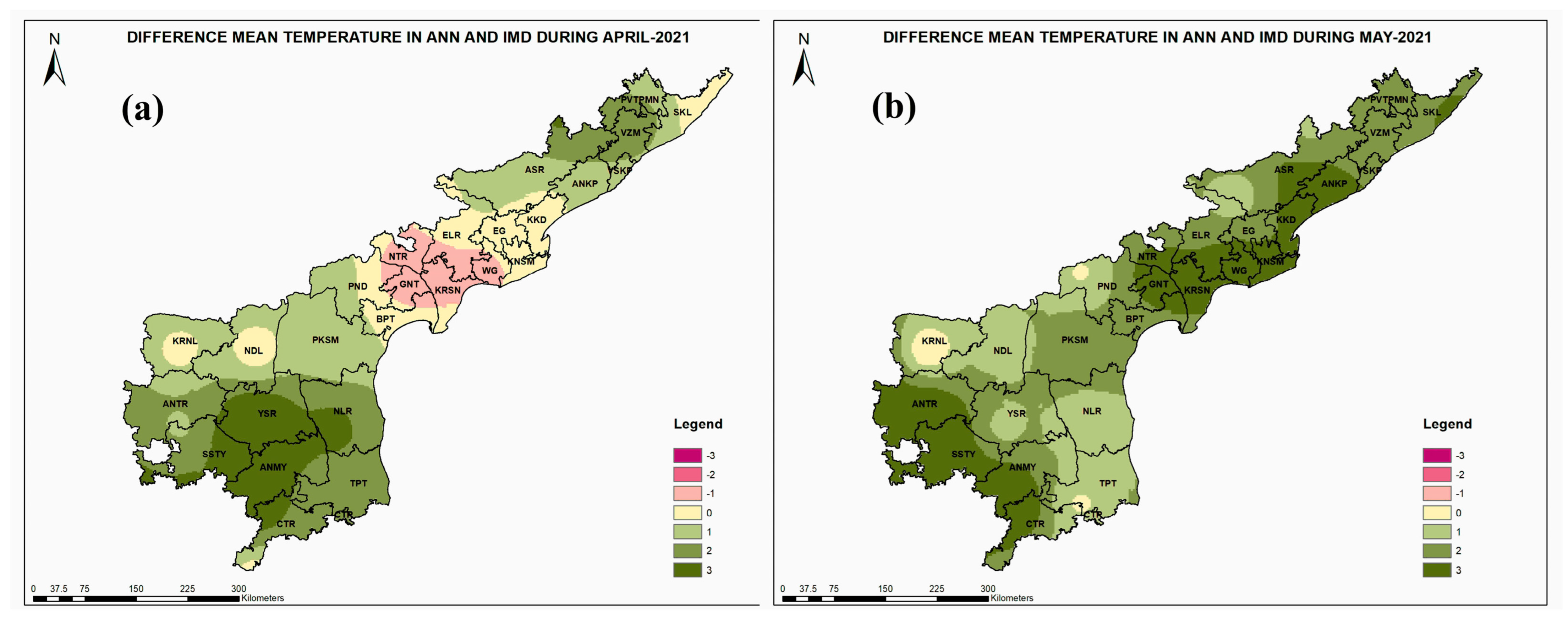
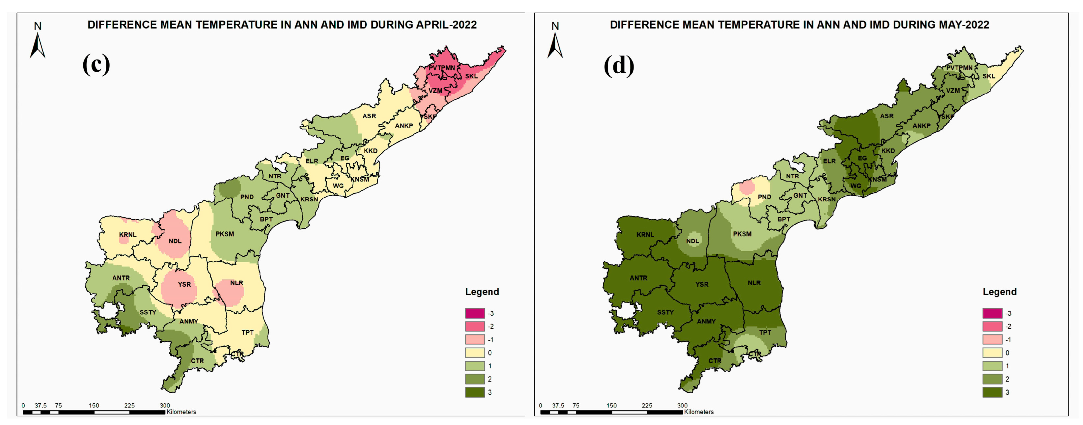
3. Results
4. Conclusions
Author Contributions
Funding
Institutional Review Board Statement
Informed Consent Statement
Data Availability Statement
Acknowledgments
Conflicts of Interest
References
- Bhadram, C.V.; Amatya, B.V.; Pant, G.B.; Kumar, K.K. Heat waves over Andhra Pradesh: A case study of summer 2003. Mausam 2005, 56, 385–394. [Google Scholar] [CrossRef]
- Climate Change 2021—The Physical Science Basis; Climate Change and Law Collection; Cambridge University Press: Cambridge, UK; New York, NY, USA, 2021.
- Krishnan, R.; Sanjay, J.; Gnanaseelan, C.; Mujumdar, M.; Kulkarni, A.; Chakraborty, S. Correction to: Assessment of Climate Change over the Indian Region. In Assessment of Climate Change over the Indian Region; Springer: Singapore, 2021. [Google Scholar]
- Solomon, S. Climate Change 2007: The Physical Science Basis; Cambridge University Press: Cambridge, UK, 2008. [Google Scholar]
- Trenberth, K.E.; Jones, P.D.; Ambenje, P.; Bojariu, R.; Easterling, D.; Klein Tank, A.; Parker, D.; Rahimzadeh, F.; Renwick, J.A.; Rusticucci, M.; et al. Observations: Surface and Atmospheric Climate Change. In Climate Change 2007: The Physical Science Basis. Contribution of Working Group I to the Fourth Assessment Report of the Intergovernmental Panel on Climate Change; Solomon, S., Qin, D., Manning, M., Chen, Z., Marquis, M., Averyt, K.B., Tignor, M., Miller, H.L., Eds.; Cambridge University Press: Cambridge, UK; New York, NY, USA, 2007. [Google Scholar]
- Vieira, F.F.; Oliveira, M.; Sanfins, M.A.; Garção, E.; Dasari, H.; Dodla, V.; Satyanarayana, G.C.; Costa, J.; Borges, J.G. Statistical analysis of extreme temperatures in India in the period 1951–2020. Theor. Appl. Climatol. 2023, 152, 473–520. [Google Scholar] [CrossRef]
- Jumin, E.; Zaini, N.; Ahmed, A.N.; Abdullah, S.; Ismail, M.; Sherif, M.; Sefelnasr, A.; El-Shafie, A. Machine learning versus linear regression modelling approach for accurate ozone concentrations prediction. Eng. Appl. Comput. Fluid Mech. 2020, 14, 713–725. [Google Scholar] [CrossRef]
- Ehteram, M.; Ahmed, A.N.; Latif, S.D.; Huang, Y.F.; Alizamir, M.; Kisi, O.; Mert, C.; El-Shafie, A. Design of a hybrid ann multi-objective whale algorithm for suspended sediment load prediction. Environ. Sci. Pollut. Res. 2020, 28, 1596–1611. [Google Scholar] [CrossRef]
- Sapitang, M.; Ridwan, W.M.; Faizal Kushiar, K.; Najah Ahmed, A.; El-Shafie, A. Machine learning application in reservoir water level forecasting for Sustainable Hydropower Generation Strategy. Sustainability 2020, 12, 6121. [Google Scholar] [CrossRef]
- Tsonis, A.A.; Swanson, K.L. Topology and predictability of El Niño and La Niña Networks. Phys. Rev. Lett. 2008, 100, 228502. [Google Scholar] [CrossRef]
- Yamasaki, K.; Gozolchiani, A.; Havlin, S. Climate networks around the globe are significantly affected by El Niño. Phys. Rev. Lett. 2008, 100, 228501. [Google Scholar] [CrossRef]
- Stolbova, V.; Surovyatkina, E.; Bookhagen, B.; Kurths, J. Tipping elements of the Indian Monsoon: Prediction of onset and withdrawal. Geophys. Res. Lett. 2016, 43, 3982–3990. [Google Scholar] [CrossRef]
- Nooteboom, P.D. Interactive comment on “Using network theory and machine learning to predict El Niño” by Peter D. Nooteboom et al. Earth Syst. Dynam. Discuss. 2018. [Google Scholar] [CrossRef]
- Dijkstra, H.A.; Petersik, P.; Hernández-García, E.; López, C. The application of machine learning techniques to improve El Niño prediction skill. Front. Phys. 2019, 7, 153. [Google Scholar] [CrossRef]
- Ratnam, J.V.; Dijkstra, H.A.; Behera, S.K. A machine learning based prediction system for the Indian Ocean Dipole. Sci. Rep. 2020, 10, 284. [Google Scholar] [CrossRef] [PubMed]
- Pal, M.; Maity, R.; Ratnam, J.V.; Nonaka, M.; Behera, S.K. Long-lead prediction of ENSO Modoki index using machine learning algorithms. Sci. Rep. 2020, 10, 365. [Google Scholar] [CrossRef] [PubMed]
- Maity, R.; Chanda, K.; Dutta, R.; Ratnam, J.V.; Nonaka, M.; Behera, S. Contrasting features of hydroclimatic teleconnections and the predictability of seasonal rainfall over East and West Japan. Meteorol. Appl. 2020, 27, e1881. [Google Scholar] [CrossRef]
- Cifuentes, J.; Marulanda, G.; Bello, A.; Reneses, J. Air temperature forecasting using Machine Learning Techniques: A Review. Energies 2020, 13, 4215. [Google Scholar] [CrossRef]
- Fan, J.; Meng, J.; Ludescher, J.; Chen, X.; Ashkenazy, Y.; Kurths, J.; Havlin, S.; Schellnhuber, H.J. Statistical physics approaches to the complex Earth System. Phys. Rep. 2021, 896, 1–84. [Google Scholar] [CrossRef] [PubMed]
- Jain, S.; Rathee, S.; Kumar, A.; Sambasivam, A.; Boadh, R.; Choudhary, T.; Kumar, P.; Kumar Singh, P. Prediction of temperature for various pressure levels using ann and multiple linear regression techniques: A case study. Mater. Today Proc. 2022, 56, 194–199. [Google Scholar] [CrossRef]
- Hanoon, M.S.; Ahmed, A.N.; Zaini, N.; Razzaq, A.; Kumar, P.; Sherif, M.; Sefelnasr, A.; El-Shafie, A. Developing machine learning algorithms for meteorological temperature and humidity forecasting at Terengganu state in Malaysia. Sci. Rep. 2021, 11, 18935. [Google Scholar] [CrossRef]
- Heng, S.Y.; Ridwan, W.M.; Kumar, P.; Ahmed, A.N.; Fai, C.M.; Birima, A.H.; El-Shafie, A. Artificial neural network model with different backpropagation algorithms and meteorological data for solar radiation prediction. Sci. Rep. 2022, 12, 10457. [Google Scholar] [CrossRef]
- Sailor, D.J.; Smith, M.; Hart, M. Climate Change Implications for Wind Power Resources in the Northwest United States. Renew. Energy 2008, 33, 2393–2406. [Google Scholar] [CrossRef]
- Pryor, S.C.; Barthelmie, R.J. Climate Change Impacts on Wind Energy: A Review. Renew. Sustain. Energy Rev. 2010, 14, 430–437. [Google Scholar] [CrossRef]
- Cradden, L.C.; Harrison, G.P.; Chick, J.P. Will Climate Change Impact on Wind Power Development in the UK? Clim. Change 2012, 115, 837–852. [Google Scholar] [CrossRef]
- Fant, C.; Adam Schlosser, C.; Strzepek, K. The Impact of Climate Change on Wind and Solar Resources in Southern Africa. Appl. Energy 2016, 161, 556–564. [Google Scholar] [CrossRef]
- Taylor, K.E.; Stouffer, R.J.; Meehl, G.A. An Overview of CMIP5 and the Experiment Design. Bull. Am. Meteorol. Soc. 2012, 93, 485–498. [Google Scholar] [CrossRef]
- Mohan, S.; Bhaskaran, P.K. Evaluation and Bias Correction of Global Climate Models in the CMIP5 over the Indian Ocean Region. Environ. Monit. Assess. 2019, 191, 806. [Google Scholar] [CrossRef] [PubMed]
- Naveena, N.; Satyanarayana, G.C.; Rao, D.V.B.; Srinivas, D. An Accentuated “Hot Blob” over Vidarbha, India, during the Pre-Monsoon Season. Nat. Hazards 2020, 105, 1359–1373. [Google Scholar] [CrossRef]
- Satyanarayana, G.C.; Rao, D.V.B. Phenology of Heat Waves over India. Atmos. Res. 2020, 245, 105078. [Google Scholar] [CrossRef]
- Singh, S.; Mall, R.K.; Dadich, J.; Verma, S.; Singh, J.V.; Gupta, A. Evaluation of cordex- South Asia regional climate models for heat wave simulations over India. Atmospheric Research 2021, 248, 105228. [Google Scholar] [CrossRef]
- Astsatryan, H.; Grigoryan, H.; Poghosyan, A.; Abrahamyan, R.; Asmaryan, S.; Muradyan, V.; Tepanosyan, G.; Guigoz, Y.; Giuliani, G. Air temperature forecasting using artificial neural network for Ararat Valley. Earth Sci. Inform. 2021, 14, 711–722. [Google Scholar] [CrossRef]
- Copernicus Climate Change Service, Climate Data Store, (2021): In Situ Total Column Ozone and Ozone Soundings from 1924 to Present from the World Ozone and Ultraviolet Radiation Data Centre. Copernicus Climate Change Service (C3S) Climate Data Store (CDS). 2021. Available online: https://climate.copernicus.eu/ (accessed on 11 November 2022).
- Srivastava, A.K.; Rajeevan, M.; Kshirsagar, S.R. Development of a High Resolution Daily Gridded Temperature Data Set (1969–2005) for the Indian Region. Atmos. Sci. Lett. 2009, 10, 249–254. [Google Scholar] [CrossRef]
- Swain, D.; Ali, M.M.; Weller, R.A. Estimation of mixed-layer depth from surface parameters. J. Mar. Res. 2006, 64, 745–758. [Google Scholar] [CrossRef]
- Badran, F.; Thiria, S.; Crepon, M. Wind ambiguity removal by the use of neural network techniques. J. Geophys. Res. 1991, 96, 20521. [Google Scholar] [CrossRef]
- Butler, C.T.; Meredith, R.v.Z.; Stogryn, A.P. Retrieving atmospheric temperature parameters from DMSP SSM/T-1 data with a neural network. J. Geophys. Res. Atmos. 1996, 101, 7075–7083. [Google Scholar] [CrossRef]
- French, M.N.; Krajewski, W.F.; Cuykendall, R.R. Rainfall forecasting in space and time using a neural network. J. Hydrol. 1992, 137, 1–31. [Google Scholar] [CrossRef]
- Ali, M.M. Estimation of ocean subsurface thermal structure from surface parameters: A neural network approach. Geophys. Res. Lett. 2004, 31, L20308. [Google Scholar] [CrossRef]
- Jain, S.; Ali, M.M. Estimation of sound speed profiles using artificial neural networks. IEEE Geosci. Remote Sens. Lett. 2006, 3, 467–470. [Google Scholar] [CrossRef]
- Krasnopolsky, V.M.; Breaker, L.C.; Gemmill, W.H. A neural network as a nonlinear transfer function model for retrieving surface wind speeds from the Special Sensor Microwave Imager. J. Geophys. Res. 1995, 100, 11033–11045. [Google Scholar] [CrossRef]
- Krasnopolsky, V.M.; Schiller, H. Some neural network applications in environmental sciences. part I: Forward and inverse problems in geophysical remote measurements. Neural Netw. 2003, 16, 321–334. [Google Scholar] [CrossRef]
- Ray, R.D.; Koblinsky, C.J.; Beckley, B.D. On the Effectiveness of Geosat Altimeter Corrections. Int. J. Remote Sens. 1991, 12, 1979–1984. [Google Scholar] [CrossRef]
- Wilks, D.S. Statistical Methods in the Atmospheric Sciences; Elsevier: Amsterdam, The Netherlands, 2006. [Google Scholar]


| MAPE | RMSE | CC | BIAS | IOA | SI (%) | Observed Mean | Predicted Mean | |
|---|---|---|---|---|---|---|---|---|
| GFDL-ESM-2G | 6.21 | 2.46 | 0.18 | −0.53 | 0.49 | 7.75 | 31.72 | 31.18 |
| ANN | 2.75 | 1.12 | 0.79 | 0 | 0.87 | 3.53 | 31.72 | 31.73 |
| MAPE | RMSE | CC | BIAS | IOA | SI (%) | Observed Mean | Predicted Mean | |
|---|---|---|---|---|---|---|---|---|
| Test-1 (1–10 day period) | ||||||||
| Training | 2.68 | 1.09 | 0.8 | 0 | 0.88 | 3.43 | 31.72 | 31.72 |
| Testing | 2.89 | 1.18 | 0.77 | 0.02 | 0.86 | 3.71 | 31.73 | 31.74 |
| Validation | 2.93 | 1.22 | 0.74 | 0 | 0.85 | 3.84 | 31.73 | 31.73 |
| Test-2 (2–10 day period) | ||||||||
| Training | 2.77 | 1.12 | 0.79 | 0 | 0.87 | 3.53 | 31.72 | 31.72 |
| Testing | 2.95 | 1.19 | 0.77 | 0.02 | 0.86 | 3.75 | 31.73 | 31.74 |
| Validation | 2.99 | 1.23 | 0.74 | 0.02 | 0.84 | 3.87 | 31.73 | 31.71 |
| Test-3 (3–10 day period) | ||||||||
| Training | 2.87 | 1.16 | 0.77 | 0 | 0.86 | 3.65 | 31.72 | 31.72 |
| Testing | 2.97 | 1.21 | 0.75 | 0.01 | 0.85 | 3.81 | 31.73 | 31.73 |
| Validation | 3.01 | 1.23 | 0.74 | −0.02 | 0.84 | 3.87 | 31.73 | 31.72 |
| Test-4 (4–10 day period) | ||||||||
| Training | 2.86 | 1.16 | 0.77 | 0 | 0.86 | 3.65 | 31.72 | 31.72 |
| Testing | 2.95 | 1.21 | 0.76 | −0.01 | 0.85 | 3.81 | 31.73 | 31.72 |
| Validation | 3.01 | 1.25 | 0.73 | −0.01 | 0.84 | 3.93 | 31.73 | 31.72 |
| Test-5 (5–10 day period) | ||||||||
| Training | 2.94 | 1.19 | 0.75 | 0 | 0.84 | 3.75 | 31.72 | 31.72 |
| Testing | 3.04 | 1.23 | 0.74 | 0 | 0.84 | 3.87 | 31.73 | 31.73 |
| Validation | 3.04 | 1.26 | 0.72 | 0 | 0.83 | 3.97 | 31.73 | 31.73 |
| Different Ranges in °C | MAPE | RMSE | CC | BIAS | IOA | SI (%) | Observed Mean | Predicted Mean |
|---|---|---|---|---|---|---|---|---|
| 34–36 °C | 3.41 | 1.35 | 0.37 | −0.97 | 0.42 | 3.89 | 34.68 | 33.71 |
| 32–34 °C | 2.63 | 1.09 | 0.36 | −0.43 | 0.51 | 3.32 | 32.83 | 32.40 |
| 30–32 °C | 2.34 | 0.98 | 0.32 | 0.16 | 0.54 | 3.15 | 31.09 | 31.25 |
| 28–30 °C | 3.76 | 1.42 | 0.27 | 0.95 | 0.41 | 4.85 | 29.24 | 30.19 |
Disclaimer/Publisher’s Note: The statements, opinions and data contained in all publications are solely those of the individual author(s) and contributor(s) and not of MDPI and/or the editor(s). MDPI and/or the editor(s) disclaim responsibility for any injury to people or property resulting from any ideas, methods, instructions or products referred to in the content. |
© 2023 by the authors. Licensee MDPI, Basel, Switzerland. This article is an open access article distributed under the terms and conditions of the Creative Commons Attribution (CC BY) license (https://creativecommons.org/licenses/by/4.0/).
Share and Cite
Satyanarayana, G.C.; Sambasivarao, V.; Yasaswini, P.; Ali, M.M. Estimating Daily Temperatures over Andhra Pradesh, India, Using Artificial Neural Networks. Atmosphere 2023, 14, 1501. https://doi.org/10.3390/atmos14101501
Satyanarayana GC, Sambasivarao V, Yasaswini P, Ali MM. Estimating Daily Temperatures over Andhra Pradesh, India, Using Artificial Neural Networks. Atmosphere. 2023; 14(10):1501. https://doi.org/10.3390/atmos14101501
Chicago/Turabian StyleSatyanarayana, Gubbala Ch., Velivelli Sambasivarao, Peddi Yasaswini, and Meer M. Ali. 2023. "Estimating Daily Temperatures over Andhra Pradesh, India, Using Artificial Neural Networks" Atmosphere 14, no. 10: 1501. https://doi.org/10.3390/atmos14101501
APA StyleSatyanarayana, G. C., Sambasivarao, V., Yasaswini, P., & Ali, M. M. (2023). Estimating Daily Temperatures over Andhra Pradesh, India, Using Artificial Neural Networks. Atmosphere, 14(10), 1501. https://doi.org/10.3390/atmos14101501