Abstract
The large eddy simulation (LES) code Fluidity was used to simulate the dispersion of NOx traffic emissions along a road in London. The traffic emissions were represented by moving volume sources, one for each vehicle, with time-varying emission rates. Traffic modelling software was used to generate the vehicle movement, while an instantaneous emissions model was used to calculate the NOx emissions at 1 s intervals. The traffic emissions were also modelled as a constant volume source along the length of the road for comparison. A validation of Fluidity against wind tunnel measurements is presented before a qualitative comparison of the LES concentrations with measured roadside concentrations. Fluidity showed an acceptable comparison with the wind tunnel data for velocities and turbulence intensities. The in-canyon tracer concentrations were found to be significantly different between the wind tunnel and Fluidity. This difference was explained by the very high sensitivity of the in-canyon tracer concentrations to the precise release location. Despite this, the comparison showed that Fluidity was able to provide a realistic representation of roadside concentration variations at high temporal resolution, which is not achieved when traffic emissions are modelled as a constant volume source or by Gaussian plume models.
1. Introduction
Personal exposure studies which use high time resolution sensors show that concentrations of harmful pollutants such as NO2 and Ultrafine Particles (UFP) are highly variable at second-by-second time scales, e.g., see [1,2,3]. Pedestrian exposure analyses are often based on the time averaged mean concentration over longer time periods, typically no shorter than an hour. These mean concentrations are often based on ambient measurements from a fixed location, or on modelled values at lower resolution which are not able to resolve highly local hotspots. For example, advanced Gaussian plume models with additional features such as a street canyon model have become the go to tool for modelling air quality in urban areas, e.g., [4,5]. These models have many advantages, e.g., providing concentration estimates at sufficient accuracy for the majority of applications, at low computational cost, while also being quick and easy to set up. However Gaussian plume models are designed to estimate time-averaged concentrations over periods of an hour or longer. Concentrations estimated using these models over shorter time periods are not necessarily meaningful, particularly when the pollutant source is highly variable.
Exposure studies therefore often fail to account for acute exposures at timescales shorter than an hour, which can occur at concentration hotspots such as busy junctions, where pedestrians may wait to cross the road, e.g., [6,7]. These hotspot concentrations vary in time due to the variation in vehicle emissions, in addition to the continually changing meteorological conditions, therefore a high spatial resolution model without an equivalent temporal resolution will not fully characterise the exposure at these locations. Further, Apte et al. (2017) [8] used mobile monitoring to demonstrate how transient peaks are responsible for the majority of the mean black carbon and NO concentrations measured along the road, while for NO2 the contribution was somewhat lower but still significant. A better understanding of these peaks, where and when they occur and how they contribute to overall exposure is required.
Computational Fluid Dynamics (CFD) large eddy simulation (LES) models are able to simulate urban airflows and the corresponding dispersion of emissions at high temporal and spatial resolution. As computer technology improves, LES is increasingly used for urban dispersion problems, for example [9,10,11,12]. LES simulations can be used in conjunction with other, less resource intensive models using a multiscale approach where the use of LES is limited to a small area of particular interest, for example [13,14]. By resolving the fine flow structures within the street, LES models are able to provide high resolution concentration fields of harmful pollutants down to length scales in the order of < 1 m and timescales < 1 s. These models can therefore be used to investigate how representative longer term mean concentration estimates are of the actual second-by-second exposure experienced by pedestrians. Fluidity is a multipurpose open source LES code with mesh adaptivity technology. Here we use the mesh adaptivity capability to automatically refine the computational mesh in the vicinity of building surfaces, where a higher degree of refinement is required to accurately capture the near surface airflow. A traffic module was developed allowing Fluidity to simulate the impact of moving vehicles on the street-level airflow and their effect on the dispersion of tailpipe emissions, represented as volume sources [15]. Here the Fluidity traffic model is used to simulate moving vehicle tailpipe emissions only, emitting NOx at time-varying emission rates. The traffic flow model is used to simulate the vehicle dynamics as they travel along the road, and an instantaneous emissions model representative of the current UK traffic fleet is used to simulate the emission rates [16]. Each vehicle tailpipe is discretely represented and we define the length of the volume source as a function of the vehicle velocity in order to ensure a smooth and continuous release as the vehicle moves along the street. This provides a high spatial and temporal resolution model of the dispersion of NOx emissions along a road in London. A similar approach was used using Reynolds-Averaged Navier–Stokes (RANS) CFD in [6,17] where traffic flow simulators were coupled to an instantaneous emissions model and used to generate time varying emissions for segments along the road. These examples achieve a high spatial resolution of both traffic emissions (down to a few metres) and pollutant concentrations, however the use of RANS means that concentration fluctuations are not captured at high time resolution unless an additional concentration fluctuations equation is solved. Other examples of CFD studies of urban air quality at the microscale typically use hourly averaged emissions, released using a constant line source along each road, e.g., [11,18,19,20]. To the authors’ knowledge, up until now there is no example of a high resolution traffic emissions model coupled with LES, providing pollutant concentration fluxes within the street at a time resolution in the order of 1 s.
A qualitative comparison is made between the model concentrations and measured data at the roadside captured during a field study in 2019. The purpose of this comparison is to demonstrate Fluidity’s ability to provide realistic roadside concentrations, which is only possible when modelling the traffic emissions at high spatial and temporal resolution. A comparison is also made with the traffic emissions modelled as a volume source of constant emission rate along the road.
Before the full scale simulations of the road are modelled, a comparison is made between the LES and wind tunnel data gathered at the University of Surrey’s EnFlo laboratory [21]. This comparison serves as a validation of Fluidity in simulating a realistic urban airflow and tracer dispersion.
2. Methodology
2.1. LES Comparison with Wind Tunnel
Before running the full scale simulations of the dispersion of traffic emissions along the road, a comparison of Fluidity with a wind tunnel simulation of the same geometry was carried out. The goal of the comparison was to ensure the quality of the LES simulations and to check that the mesh configuration used was adequate to provide a reasonable representation of the airflow.
2.1.1. Wind Tunnel Simulation
The wind tunnel simulation was carried out at the EnFlo laboratory at the University of Surrey [21]. The geometry used was a 1:200 scale model of an area in south London, centred on London Road in the borough of Southwark. The area used consists of the buildings along London Road in addition to some surrounding buildings away from the road. The model was placed within a simulated neutral boundary layer flow within the wind tunnel. The buildings included in the wind tunnel correspond to those seen in Figure 1. A two-component Laser Doppler Anemometer was used to measure flow velocities and turbulence intensities with a sampling rate of 100 Hz. Propane mixed in a passive carrier was used as a passive tracer gas and released near the west end of London Road as a diffuse release (see Figure 1). A single Fast Flame Ionisation Detector, with a sampling rate in the order of 200 Hz, measured the tracer concentration at three cross-sectional planes, A, B and C (Figure 1), of London Road from a height range of Z = 0.011– m (equivalent to 2.2– m at full scale).
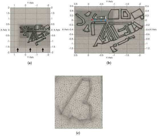
Figure 1.
LES mesh configuration for wind tunnel simulation. Dimensions are shown in metres and the domain height was set to the height of the wind tunnel, H = 2 m. (a) LES mesh for wind tunnel simulation, the full extent of the domain is shown, (b) Location of tracer source (red circle) and measurement planes (blue lines), (c) Mesh refinement at a building facade.
Three points should be emphasised here:
- The full wind tunnel model consisted of around 100 buildings, but the model used here is a cut-down version that was used in an investigation of the response of flow and dispersion in London Road to the extent of the model. The consequence of this is that the LES runs required a smaller computational resource than would be demanded for the full model.
- The source location, shown in Figure 1, is in a position where sensitivity to precise location is expected to have a significant impact on dispersion behaviour, in particular the division of fluxes between the surrounding streets (the location is actually a roundabout). As will become apparent, this is not ideal for evaluating the ability of the LES model to predict dispersion. The specified source location and wind direction, indicated by the arrows in Figure 1, provides a particularly strong test of predictive ability for the tracer concentration along London Road; being perpendicular to the road, the oncoming wind can only generate flow along the road because of the interplay between the approaching flow and the heterogeneous geometry. A number of other data sets were available for the full model but these are not used here in favour of a case which is computationally less intensive. However, previous studies have shown that Fluidity is able to simulate tracer dispersion in urban settings with reasonable accuracy [22,23,24]. This is an additional case which tests the particular meshing method used and provides further assurance of the quality of Fluidity’s predictions.
- We are concerned with Fluidity’s ability to accurately replicate the flow statistics and tracer concentrations within the street canyon specifically. We therefore validate Fluidity against the X and Z direction components of the velocity and turbulence fields. The wind direction, perpendicular to the street, provides the strongest statistics in these two directions making it easier to compare the statistics derived from the two models. Given the sensitivity of the tracer concentrations within the canyon to the exact source location, we use two separate methods to normalise the concentrations. The first is commonly used in wind tunnel and CFD studies:where C is the tracer concentration, is the reference wind velocity, H is the height of the boundary layer and Q is the emission rate.
For the second normalisation we divide by the mean tracer concentration at measurement plane A such that,
where is the mean of the concentrations for all measurement points at plane A and all timesteps, and is the equivalent for the LES simulation. This is used as an approximation to normalising by the amount of tracer entering the street canyon.
2.1.2. LES
Fluidity is an open-source software developed at Imperial College London (https://fluidityproject.github.io/ (accessed on 1 July 2022). It is a general purpose, finite element CFD software within which a LES methodology is implemented with an anisotropic adaptive mesh. Using LES, Fluidity is able to simulate unsteady flows, resolving turbulent features of the flow larger than a specified filter length by solving filtered Navier–Stokes equations. Turbulent eddies smaller than the filter length are modelled as additional viscosity based on a Smagorinsky-type model. Its adaptive mesh capability allows Fluidity to resolve the mesh in response to flow features, for example resolving regions of high gradients while using a coarse mesh in stable regions. The level of refinement is controlled by an user defined interpolation error and minimum and maximum edge lengths. For more detail on the adaptive mesh technology see [25].
Incompressible Navier–Stokes equations are solved to calculate the velocity and pressure fields as follows
Here and are the resolved velocity and pressure fields, occurring at length scales above the filter length, and is the density of the incompressibel fluid. The kinematic viscosity of the fluid is given by , while represents the eddy viscosity. A continuous Galerkin discretization and a Crank-Nicholson scheme were used to discretise in space and time, respectively, and a fixed time step of s was used.
The passive tracer release was represented as a volume source, the dispersion of which is modelled using an advection-diffusion equation, as follows
where C is the tracer concentration, is the diffusivity tensor and F is a source term. This equation is discretized using a second-order coupled finite element/control volume method. For more detail see [15,22,23].
A turbulent velocity profile was applied at the domain inlet using the Synthetic Eddy Method [22,26]. The simulated neutral boundary layer profile measured in the wind tunnel was used to set the X, Y and Z velocity (u, v, w) and turbulence intensity (, , ) components (see Figure S1). A wind speed of 2 ms-1 was set at a height of 1 m from the ground to match that of the wind tunnel.
A near-wall log law boundary condition was applied at all surfaces, including building surfaces, while a zero pressure condition was applied at the domain outlet.
2.1.3. Mesh Configuration
A minimum edge length of m was set for the domain (equivalent to m at full scale). Away from London Road, the location of the tracer release and wind tunnel measurement points, the maximum edge length was set to m (10 m full scale equivalent). This maximum element length scale was progressively reduced around the buildings and was set to m along much of London Road itself.
A scalar field was defined with a value of 1 at the building facades and 0 elsewhere. The simulation was then let to run with Fluidity adapting the mesh both to the velocity and to the building facade scalar field. The result was a mesh of 1.2 million nodes, with a refined mesh around the buildings, particularly at the leading edges as seen in Figure 1. Once satisfied with the mesh the adaptivity was turned off and the simulation continued.
2.1.4. Performance Criteria for LES
We use the acceptance criteria proposed by Hanna and Chang [27] to evaluate the performance of the model, as done in COST 732 [28] and COST ES1006 [29]. Hanna and Chang’s criteria are as follows:
- ≤ 0.3 —The relative Fractional Bias (FB) is less than or equal to 0.3.
- NMSE ≤ 3.0 —The Normalised Mean Square Error (NMSE) is less than or equal to 3.
- FAC2 ≥ 0.5—The fraction of predicted values, P, within a factor of two (FAC2) of the observed values, O, is greater than or equal to 0.5.
- NAD ≤ 0.3—The Normalised Absolute Difference (NAD) is less than or equal to 0.3.
The mathematical definition for each performance measure is given in the Appendix A.
While these criteria were proposed to evaluate the maximum concentration along an arc, we apply them to a point-by-point comparison, therefore our spatially constrained comparison is more stringent. Time averaged mean values are used for the comparison at each point. For the LES these time averaged mean values were derived from the duration of the simulation, excluding an initial spin up period, equalling approximately 30 s (equivalent to 100 min at full scale). The wind tunnel simulation was able to run for a significantly longer time period resulting in time averages calculated over approximately 3 min.
We also use the hit rate, HR, as a criteria where HR is given by:
Here, and are the predicted and observed time-averaged concentrations, respectively, n is the total number of observed concentrations and N is the total number of the predicted concentrations which satisfy the criteria.
For the allowed relative deviation, D, we use 0.25, as done in COST 732 [28]. For the allowed absolute deviation, W, rather than use a single fixed value for all points, we use a value derived for each individual point of comparison. The duration of the simulation in the wind tunnel was considerably longer than that for the LES (roughly 3 min for the wind tunnel and 40 s for the LES), mainly due to limitations on computational run time. In order to calculate W, we divided the wind tunnel data (approximately 3 min) into time periods equivalent to that generated by the LES simulation (approximately 30 s), calculating the velocity and turbulence statistics for each separate time period. We then defined W as the maximum difference between these values. This provides an estimate of the repeatability of the results at each point. An illustration of W for a single point is given in the Supplementary Material (Figure S2). This method of deriving W leads to a more stringent criteria, with generally much lower values of W, than those used in the VDI guideline [30] where a 0.66 acceptance limit is proposed for HR.
We also extend the criteria to the velocity and turbulence statistics.
2.2. Full Scale Simulations
The method used to simulate the concentrations along London Road consists of three parts: the modelling of vehicle movement for traffic along the road, the modelling of the second-by-second emissions of each individual vehicle, and the modelling of the dispersion of the traffic tailpipe emissions. This process is summarised in Figure 2.
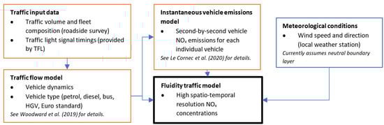
Figure 2.
Flow chart of methodology used to simulate high spatio-temporal NOx concentrations from traffic emissions. TFL stands for Transport for London.
Manual vehicle counts collected in June 2019 were used to configure the traffic flow model, while weather data collected was used to define the velocity and turbulence profiles at the LES inlet. The goal was to replicate two hour-long periods during two separate days of the field study (the 20 September and 27 September 2019) in order to make a qualitative comparison of the measured and simulated data. These two days and associated simulations are referred to as Day 1 and Day 2.
The sensors used during the field study that provided the data and used to compare with the LES were a M200E Chemiluminescence analyser by Teledyne Instruments [31], measuring NOx and NO2 at a 1 min resolution, and a Serinus 60 NO analyser using cavity attenuated phase shift spectroscopy (CAPS) to measure NO2 at a 1 s resolution (the rise and fall time of this instrument is 30 s) [32]. The locations of these sensors are shown in Figure 3. A background subtraction has been applied to the measured values shown in this paper unless stated otherwise. The background subtraction assumes a value for the “background” signal (i.e., concentrations emanating from other sources away from the road) equal to the minimum measured concentration over a rolling 4 min window. This method is similar to that used by [33] for a network of sensors, however here is only applied to a single sensor. The restriction of only one sensor of course limits the utility of this method, however sensitivity studies and comparisons with nearby reference background measurements revealed that the method was sufficient for its purpose. The result is an approximation of the concentration signal due to the emissions from the road only.
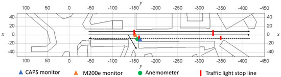
Figure 3.
Location of monitors along London Road for the field study. The black arrows indicate lanes of traffic. The dashed line indicates a bus lane. Dimensions are shown in metres.
2.2.1. Traffic Movement Modelling
The commercial software PTV Vissim [34] was used to simulate the traffic flow along London Road. PTV Vissim is primarily used for traffic management purposes and is able to simulate the movement of each individual vehicle that travels along the road. The software was used in [15] to simulate the traffic flow and resulting emissions for an idealised crossroads, and more details on its use for CFD modelling can be found there.
Hourly average traffic counts were used as input to the model, with the number of cars, LGVs, buses and HGVs all specified. A petrol/diesel split for passenger cars was applied based on National Atmospheric Emissions Inventory (NAEI) data. The simulations generated 3600 s of second-by-second output data for the two study days, consisting of location, speed and acceleration for each vehicle along the road.
2.2.2. Traffic Emissions Model
The NLR model developed by [16] was used to generate second-by-second NOx data for each simulated vehicle. The model draws on emission datasets for petrol and diesel passenger cars, LGVs, HGVs and buses for a range of Euro categories. A Euro category mix based on the NAEI and Ultra Low Emission Zone (ULEZ) restrictions was assumed.
2.2.3. Full Scale LES Configuration
The same LES configuration as outlined in Section 2.1.2 was used for the full scale simulation with some necessary adjustments outlined below.
For the full scale simulations the domain was expanded in order to allow a greater distance between the buildings and the domain outer boundaries. The boundary edges, other than the ground, buildings, inlet and outlet, were then simulated using full slip conditions rather than wall boundary conditions. This was done in order to remove the effect of the wind tunnel walls from the full scale simulation.
Table 1 shows the wind speed measured nearby at Z = 200 m (London’s BT Tower) used to define the reference wind velocity, , and the predominant wind direction used to set the appropriate angle of the buildings to the domain inlet. The same boundary layer profile for the velocity and turbulence intensities was assumed as those of the wind tunnel, but scaled to at full scale.

Table 1.
Inlet velocity configuration for the two field study days. is the reference velocity at the domain height of 200 m.
The LES assumes a perfectly neutral flow whereas in reality a degree of convective mixing is expected. This is particularly true for Day 1 which was a clear sky day. Despite the clear sky, the reference wind velocity was considered high enough that the flow is likely not far from neutral. For Day 2 the wind speed was higher and the sky was overcast and so better characterised by a neutral boundary layer.
A fixed time step of s and s was used for the Day 1 and Day 2 simulations, respectively. A lower time step was used for Day 2 such that the mean Courant number for the simulation was similar to that of the Day 1 simulation. The same meshing approach as for the wind tunnel simulation was used, adjusting the element size range appropriately for the full scale case. An initial period of 15 min was simulated without traffic emissions in order to allow the wind flow field to develop. After this initial period an additional 45 min was simulated with traffic emissions.
2.2.4. Dynamic Traffic Emissions Modelling
The vehicle emissions were modelled as a passive tracer. Fluidity has an inbuilt traffic module capable of simulating individual vehicles and their emissions as they move through the domain, see [15] for details, while the model is able to simulate the effect of vehicles on the airflow and vehicle-induced dispersion, the inclusion of this feature adds significantly to the run time of the model. Therefore, for this study we used the model to simulate moving tailpipe emissions only, represented as moving volume sources, without simulating the vehicles themselves.
Each vehicle within the domain was assigned an individual volume source representing the tailpipe emissions. The strength of this source was set by the second-by-second emissions data provided by the NLR model, while the location at any given time was provided by the PTV Vissim model. The source size was set at a minimum of 2 m × 2 m × 2 m. The source was allowed to extend in length along the direction of travel of the vehicle such that:
where SL is the source length along the direction of travel and v is the vehicle velocity. This ensured the smooth progression of the vehicle source along the road, without skipping from one location to the next between timesteps, regardless of the vehicle velocity and simulation timestep used. Mixing of the tailpipe emission within the wake of the vehicle is also likely to increase with vehicle speed as the wake turbulence increases. This model therefore also captures, to some degree, the increased mixing along the direction of travel which is likely to occur as the vehicle is moving. We refer to this method of modelling the traffic emissions as the Dynamic Traffic Model (DTM).
A separate tracer was used for passenger vehicles, HGVs and buses, allowing the concentrations resulting from each vehicle type to be studied individually if desired. A constant volume source was also applied along London Road. This emitted a passive tracer at a constant rate from a volume m in height and the width of the road. The emission rate of the volume source was set to equal the average emission rate of the entire fleet of moving vehicles over the duration of the simulation. This method is referred to as the Volume Source (VS) method.
Figure 4 shows a snapshot of the emission sources along the road. The small red squares are the tailpipe volume sources for the vehicles travelling along the road at the time. The blue area indicates the area of the volume source.
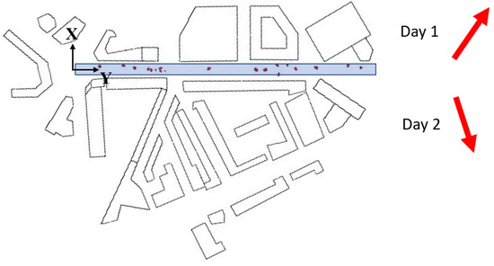
Figure 4.
A snapshot of moving vehicle sources (red) and volume source (blue) along London Road. The coordinate system, with Z vertical, is also shown. The prevailing wind direction for both days is indicated by the red arrows.
3. Results and Discussion
Before we consider the full scale simulations and the representation of traffic emissions as moving, time-varying sources, we compare the wind tunnel-scale simulation with the wind tunnel measurements.
3.1. Comparison with Wind Tunnel
3.1.1. Velocities and Turbulent Velocities
Figure 5 and Figure 6 show the comparison of the velocity and turbulence statistics simulated in the wind tunnel and by the LES. Table 2 shows a summary of the performance criteria for all points and for all points within the street canyon. Other than for the Reynolds stress, which narrowly fails for FAC2 and NAD when the comparison is constrained to the points within the street canyon, the acceptance criteria of Hanna and Chang [27] (see Section 2.1.4) are met in all cases. However, the hit rate target is in the most part not achieved. This may be due to the more stringent threshold values used for the absolute deviation, W, than that used by [30] when recommending the target HR of 0.66. It may also be due to the complex urban geometry used, for which a good agreement is a greater challenge than for regular building arrays.
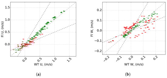
Figure 5.
Scatter plots of (a) u and (b) w for the wind tunnel and LES. Green markers indicate values which meet the criteria, red markers indicate values which do not meet the criteria. Dotted line is the x = y line, dashed lines are the factor 2 lines.
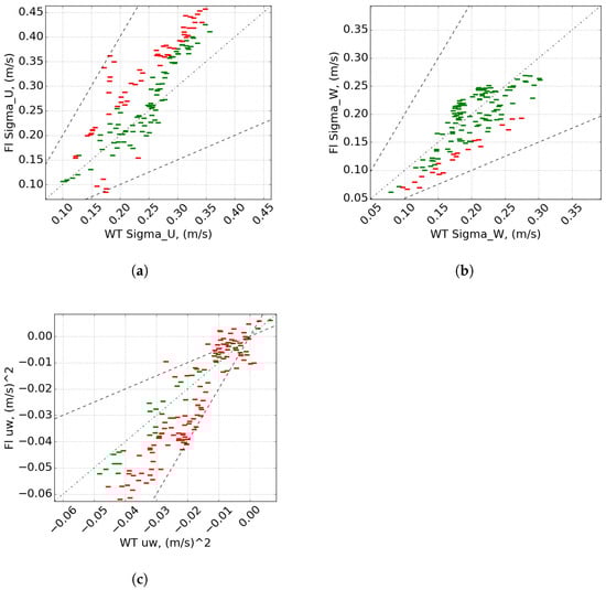
Figure 6.
Scatter plots of (a) , (b) and (c) for the wind tunnel and LES. Green markers indicate values which meet the criteria, red markers indicate values which do not meet the criteria. Dotted line is the x = y line, dashed lines are the factor 2 lines.
Table 2.
Performance statistics of LES against the WT. Values which do not reach the proposed criteria are shown in bold.
The discrepancy is also likely in part due to a lack of mesh resolution. A finer mesh is likely to improve these results. However, the objective here was to achieve a mesh which gave acceptable results with more manageable run times, rather than to obtain optimal accuracy. This echoes the choice of using data from the cut-down wind tunnel model.
The discrepancy in velocities u and w between the LES and WT occurs mainly for points at which u and w are small. The comparison is least satisfactory for the vertical component, w, which has in the most part much smaller magnitudes than u. However, the vertical turbulent velocity, , is typically an order of magnitude greater than the vertical velocity component, w, for the corresponding points and will generally dominate the vertical dispersion of any tracer. Likewise, at the locations where the streamwise velocity, u, is small, the streamwise turbulent velocity, , is typically significantly greater. The LES performs particularly well for these turbulent velocities.
3.1.2. Tracer Concentrations
While running the LES simulations it was found that the amount of tracer entrained into the street canyon was highly sensitive to the precise source location. A slight change of location of the source led to an order-of-magnitude difference in the concentrations within the street canyon. This confirmed our expectations, discussed in Section 2.1.1. This is clearly visualised by the mean streamlines shown in Figure 7, emanating from locations in the vicinity of the actual source. For the first location the origin of the streamlines is the best approximation to the location of the source within the wind tunnel. For the second and third, the origin is moved m and m in the Y direction, respectively. For the first location the majority of streamlines enter the street canyon. However for the second location a significantly different picture is seen with only a minority of streamlines entering the street canyon. For the third location none of the streamlines enter the street canyon. These are streamlines calculated from the average velocity field and, therefore, do not account for tracer dispersion due to the unsteady component of the velocity. However, they do indicate the likely sensitivity of dispersion behaviour to the precise location of a small source, and explain the large differences in concentrations seen within the canyon when the source location was moved slightly. A further factor probably lies in the precise manner in which emissions were simulated in the LES and wind tunnel. Usually, this is not an issue of concern, but given the sensitivity of dispersion behaviour to source location there is also likely to be some sensitivity to the means by which the tracer is introduced in the two media.
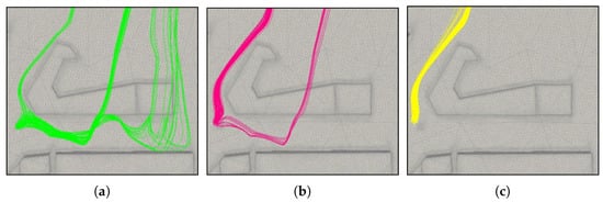
Figure 7.
Mean streamlines from the source area: (a) the location in the wind tunnel denoted by , such that ; (b) the location is shifted by 10 mm m); (c) the location is shifted by 20 mm m). The height, Z = mm, is the same for each case.
Figure 8 shows the comparison of the normalised concentrations (, Equation (1)) measured in the wind tunnel and those simulated by the LES. The LES concentrations are an order of magnitude greater than those measured in the wind tunnel. As explained above this was deemed to be due to the sensitivity of the street canyon concentrations to the location of the source, where only a small error between the relative location of the source in the wind tunnel and in the LES could lead to significant differences in concentrations.
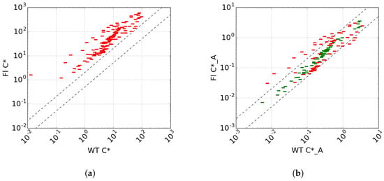
Figure 8.
Scatter plots of (a) and (b) for the wind tunnel and LES. Green markers indicate values which meet the criteria, red markers indicate values which do not meet the criteria. Dotted line is the x = y line, dashed lines are the factor 2 lines.
However, there seemed to be a worthwhile method for comparing dispersion in London Road, based on the quality of the predicted velocity and turbulence fields. This used concentrations normalised by the spatial and time-averaged concentration across the measurement plane A (, Equation (2)) as discussed in Section 2.1.1. When using this alternative normalisation a reasonable comparison was seen between the wind tunnel and LES (Figure 8). This indicates that whilst the LES failed to simulate the entrainement of tracer into the street canyon for this particular source location, for the reasons discussed above, it was able to replicate the in-canyon dispersion of the tracer with reasonable success.
Overall, these results, together with previous Fluidity evaluation studies [22,23,24], were deemed acceptable for our requirements of achieving a realistic turbulent atmospheric airflow and associated in-canyon tracer dispersion along London Road.
3.2. Full Scale Simulations
A direct, quantitative comparison between the field study and LES simulations is not meaningful for a number of reasons. First, a number of features are not considered in the LES simulations. These include street furniture, building roof shapes and the many trees planted along London Road, and the physical presence of the emitting vehicles. Further, the LES assumes a perfectly neutral flow and neglects any convective mixing, which is expected to have been present for Day 1. The street-level wind velocities for the LES were found to be significantly higher than those measured at the roadside (see Figure S3). One likely reason for this is the shortage of upwind buildings in the LES simulation, particularly for the Day 2 simulation, while a good agreement was achieved for the wind direction for Day 2, the same could not be said for Day 1 for which field study measurements revealed a complex bidirectional flow within the street canyon, similar to that observed in [35]. There are also difficulties in comparing results with data collected at a single location as values can vary significantly over very short distances at street level. Further, while the mean traffic volume used for the LES simulations were representative of those during the field study, and the traffic light signal timings were the same, the traffic flows are otherwise different. The individual vehicle emissions will also be different as the emissions model does not replicate the emissions of individual vehicles exactly. Finally, for the comparison with the CAPS sensor we are comparing modelled NOx values with measured NO2, therefore making the assumption that their signals are similar at the roadside. This assumption is supported by the similarity between the NOx and NO2 signal measured by the M200e sensor.
Despite these many considerations, a qualitative comparison is made between the simulated and measured concentrations. The objective of this comparison is to demonstrate that the LES methodology is able to capture statistics representative of the highly variable nature of the concentration field at the roadside, and provide comparable time series plots and concentration ranges.
Qualitative Comparison of Roadside Measured and Simulated Concentrations
Figure 9 shows timeseries plots of the background-subtracted measured roadside concentrations and the LES concentrations for both days and both sensor locations. Here we are comparing the LES timeseries with a 45 min segment of the full measurement period which spanned 4 h on both days. Both the VS and the DTM source concentrations are shown. The LES concentrations have been time averaged to match the effective time resolution of the sensor. For the CAPS, which provides values at 1 s intervals but has a 30 s rise and fall time, a 30 s rolling average is used. For the M200e, which has a 60 s time response, a 60 s average is used. The peak concentrations for the M200e sensor are much lower than those for the CAPS figures due to the longer averaging time used.
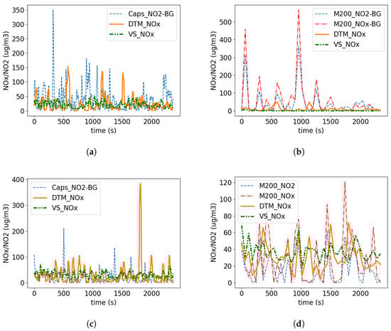
Figure 9.
Comparison of measured and modelled timeseries concentrations. (a) Day 1 CAPS (30 s rolling average), (b) Day 1 M200e (60 s average), (c) Day 2 CAPS (30 s rolling average), (d) Day 2 M200e (60 s average). The LES concentrations have been time averaged to match the time resolution of each sensor.
We reiterate that the LES and field data cannot be expected to match one another in time, because of the stochastic nature of some of the processes controlling emissions and dispersion behaviour. What we seek is a qualitative similarity and that the statistics are well modelled.
There is a strong correlation between the NOx and NO2 concentrations measured by the M200e sensor, allowing a qualitative comparison of the modelled NOx and measured NO2. The DTM and measured CAPS concentrations behave in a similar way, with both displaying semi-regular concentration peaks approximately 60 s apart, which is in the order of the time period of the traffic lights. These peaks are generated both by the idling engines of queuing vehicles and the spike in emission rates seen on acceleration when the light turns green (e.g., see [15,36]). The VS concentrations show much less variability as expected, but are not constant, despite a constant emission rate, due to the street-level turbulence.
The DTM concentrations for the M200e location for Day 1 are very low and do not show a similar behaviour to the measured signal, with very little variation (Figure 9b). The VS concentrations are also very low for the duration of the simulation. Maps of the street-level wind velocity for this simulation reveal that the sensor lies upwind of the road (Figure S4), therefore the vast majority of traffic emissions are dispersed away from it leading to very low concentrations. Significant peaks are seen for the measured data despite a similar prevailing wind direction. This is likely due to a more complex street-level wind flow than that which is simulated by the LES which does not capture effects such as wind meandering. This is likely true for Day 1 in particular for which a complex bi-directional wind flow was measured at street level and is not replicated by the LES. These peaks may also be due to the effect of vehicle movement on the street-level dispersion of tailpipe emissions, such as that highlighted by [15]. The full Fluidity traffic model, including the effect of vehicle movement on air dispersion, can be used to investigate this in future.
Figure 10 shows box plots of simulated NOx concentrations for both the VS and the DTM source, in addition to measured background-subtracted concentrations. Both the simulated and measured concentrations shown have been normalised by the time averaged mean concentration. The LES values have again been time averaged to provide a time resolution matching that of the sensor.
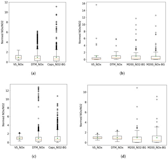
Figure 10.
Comparison of measured and modelled box plots. (a) Day 1 CAPS (30 s rolling average), (b) Day 1 M200e (60 s average), (c) Day 2 CAPS (30 s rolling average), (d) Day 2 M200e (60 s average). The green triangle indicates the mean, the orange line the median and the whiskers extend the inter-quartile range. An approximation of the background concentration has been subtracted from the measured NO2 data.
As expected the DTM captures the variation in concentrations much more successfully than the volume source. The variation that is present for the volume source is generated purely by the turbulent airflow within the street canyon. The variation in the DTM concentrations is much greater and is in the most part due to the variation in vehicle emissions. The DTM provides a good approximation of the mean, median and inter-quartile range for the CAPS sensor on both days. The comparison for the M200e sensor is somewhat less satisfactory, however is still a significant improvement as compared to the VS model. For the Day 1 M200e comparison (Figure 10b) the apparent variation in VS concentrations is artificial as the mean concentration used for the normalisation is so low.
It is interesting to note that the time averaged mean concentration (green triangle) is consistently greater than the median (orange line) for both the DTM and measured values, but not the volume source. There are also a significant number of outliers beyond the limit of the whiskers. In fact the figures do not show the full extent of these outliers for the measured data, with the maximum value reaching 2400 gm−3 for the CAPS sensor on Day 1. It is therefore clear that the concentrations are not normally distributed, and are likely more accurately represented by a log normal distribution. These high outliers are likely due to particularly dirty vehicles passing the sensors. These high emitters are not captured by the DTM because the emissions model uses emission factors representative of the mean for any particular vehicle category. Therefore, although peak emissions are captured while vehicles accelerate, the variation in the magnitude of these peaks is not fully captured.
Figure 11 shows the LES 1 s resolution timeseries concentrations and associated box plot for Day 2 at the CAPS location. The difference between the volume source (blue line) and DTM concentrations (orange line) is particularly clear for this high time resolution. A maximum 1 s NOx concentration of 3000 gm−3 is seen for the DTM tracer. At this resolution the true nature of the roadside concentrations are seen. The median concentration is very small (3 gm−3), an order of magnitude lower than the mean at 30 gm−3. The concentration experienced by a pedestrian at this location will therefore be significantly lower than the mean concentration for the majority of the time, but interjected with very short duration, very high concentration peaks reaching up to and above 3000 gm−3 (the box plot scale has been limited to 400 gm−3).
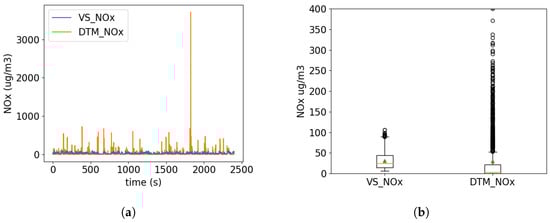
Figure 11.
LES concentrations for volume source and dynamic traffic model for Day 2 at location of CAPS sensor. (a) Day 2 time series (1 s resolution) and (b) Day 2 box plot (1 s resolution).
A lower time resolution sensor, e.g., 1 h time response, will provide an estimate of the mean concentration for the hour. However, as the mean is significantly greater than the median this will be an overestimate of shorter time duration exposures at this location in most instances. For the DTM the 1 s resolution concentrations were found to be below the mean concentration for 77.3% of the time on average across both days and both sensor locations. For the 30 s rise and fall CAPS measurements, concentrations were found to be lower than the mean value for 64.8% of the time, while for the M200e this value was 77.0% for NO2 and 73.6% for NOx. This raises the question as to how representative mean concentrations measured over longer periods at a fixed location are of pedestrian exposure along the roadside. Further, assuming the breathing cycle period while walking or cycling is in order of 1 s, the DTM results suggest that the inhaled NO2 will be highly variable about the mean.
It should be noted that the simulated values do not consider sources other than the traffic along the road. If we were to include the background signal then the concentrations would be greater and the variation in the signal relative to the mean would become somewhat less important. However, measurements taken at the roadside at 1 min resolution or lower often show a standard deviation greater than the mean. For the measurements taken here the mean, median and standard deviation values, with no background subtraction, are shown in Table 3. The median is consistently, and often significantly, lower than the mean, while the standard deviation is of the same order or greater than the mean. The LES values are also included for comparison.
Table 3.
Mean, median, standard deviation and Coefficient of Variance (CV) for the measured and modelled concentrations (g/m3). These values are total concentrations, no background subtraction has been applied to to these numbers.
Finally, Figure 12 shows a map of the time averaged mean and standard deviation of 1 s resolution concentrations along the road for Day 2. Mean concentration hotpots can be seen near the junction (Y = m) and pedestrian crossing (Y = m) where vehicles are required to stop then accelerate from standstill. These locations also correspond to where pedestrians are likely to wait to cross the road. The standard deviation map shows that the variation in concentration is often of the same order or greater than the mean. The standard deviation is also greater for a larger proportion of the road, demonstrating that while mean concentrations are much lower away from the junction and pedestrian crossing hotspots, peak concentrations occur along the entire length of the road. This behaviour was not captured by the VS representation of the traffic emissions.
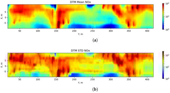
Figure 12.
Colour maps of dynamic traffic source concentration (g/m3) (a) mean values and (b) standard deviation of 1s signal along the road with wind direction of 40 deg and wind speed of 12 m/s. Values shown at a height of 1m and have been mapped to a 2 m resolution grid.
4. Conclusions
The LES model, Fluidity, has been used to simulate NOx concentrations due to traffic emissions at high time and spatial resolution along a road in London. The method used is similar to that outlined in [15], however in this case vehicle-induced dispersion is not explicitly considered. The speed-dependent effect of vehicle-induced dispersion on the initial mixing of tailpipe emissions within the vehicle wake is accounted for by using volume sources which increase in length with vehicle speed. This method also guarantees the smooth, continuous progression of tailpipe emissions along the road between simulation time steps. This method was compared both to roadside measurements and a volume source representation of the traffic emissions, which is commonly used in CFD simulations. The objective was to demonstrate that the approach could provide more realistic concentration variations within the street at timescales down to 1 s than that achieved with a constant volume source.
Before running the traffic simulation, a further validation of Fluidity was carried out against wind tunnel data. The comparison showed that Fluidity is able to provide a reasonable representation of the street-level velocity and turbulence statistics. The initial comparison of in-canyon tracer concentrations was far from satisfactory, however the high sensitivity of the in-canyon concentrations to the tracer source location was identified as an explanation. When normalised by the average concentrations entering the canyon, a satisfactory comparison was achieved.
A qualitative comparison of the Fluidity NOx concentrations and measured NOx and NO2 at the roadside demonstrated the model’s ability to replicate similar variations in concentrations, which was not achieved by the volume source concentrations. At 1 s resolution the concentration at the roadside due to the road traffic is shown to be very low but interrupted by very short duration, very high peak concentrations which raise the mean concentration significantly above the median. For the roadside location considered, the 1 s NOx concentrations were found to be below the time averaged mean value for 77% of the time, raising the question of whether the time averaged mean is the most appropriate value to use when estimating the level of harm to pedestrians. Further, the high spatial resolution map produced revealed hotspots at the junction and pedestrian crossings for both time averaged mean and standard deviation concentrations. These locations correspond to those at which pedestrians typically spend the most time at the roadside as they often wait to cross the road.
The method developed and presented here is able to capture the true nature of roadside concentrations at high temporal resolution. These highly variable concentrations with very short, very high concentration peaks at timescales down to the order of 1 s are not currently considered when evaluating pedestrian exposure at the roadside, and are not captured by commonly used models such as advanced Gaussian plume models.
Further work is planned to investigate the significance of these highly variable concentrations on pedestrian exposure when modelled at this high temporal resolution.
Supplementary Materials
The following supporting information can be downloaded at: https://www.mdpi.com/article/10.3390/atmos13081203/s1, Figure S1: Inlet velocity and turbulence; Figure S2: Illustration of derivation of the allowed absolute deviation, W; Figure S3: Wind roses showing the roadside wind speed and direction; Figure S4: Average velocity vortices at street level (Z = 1 m) as modelled by the LES for Day 1.
Author Contributions
Conceptualization, H.W., A.K.S. and M.E.J.S.; methodology, H.W., C.P., A.K.S., C.M.A.L.C.; software, H.W., C.M.A.L.C., A.K.S.; validation, H.W. and A.R.; formal analysis, H.W.; resources, H.A., A.R., M.E.J.S.; writing—original draft preparation, H.W.; writing—review and editing, A.K.S., A.R. and P.F.L.; visualization, H.W.; supervision, H.A. and M.E.J.S.; funding acquisition, H.A., C.P., A.R. and P.F.L. All authors have read and agreed to the published version of the manuscript.
Funding
This work was funded by the Engineering and Physical Sciences Research Council (EPSRC) Grand Challenge grant ‘Managing Air for Green Inner Cities (MAGIC) [grant number EP/N010221/1].
Data Availability Statement
Data are still undergoing QA processing and will be released once that is completed. Until then, data are available on request.
Conflicts of Interest
The authors declare no conflict of interest.
Appendix A
Here O denotes observed values (i.e., WT values) and P denotes predicted values (i.e., LES values). The overbar denotes the point-wise mean.
References
- Yang, F.; Kaul, D.; Wong, K.C.; Westerdahl, D.; Sun, L.; Ho, K.F.; Tian, L.; Brimblecombe, P.; Ning, Z. Heterogeneity of passenger exposure to air pollutants in public transport microenvironments. Atmos. Environ. 2015, 109, 42–51. [Google Scholar] [CrossRef]
- Borge, R.; Narros, A.; Artíñano, B.; Yagüe, C.; Gómez-Moreno, F.J.; de la Paz, D.; Román-Cascón, C.; Díaz, E.; Maqueda, G.; Sastre, M.; et al. Assessment of microscale spatio-temporal variation of air pollution at an urban hotspot in Madrid (Spain) through an extensive field campaign. Atmos. Environ. 2016, 140, 432–445. [Google Scholar] [CrossRef]
- Ham, W.; Vijayan, A.; Schulte, N.; Herner, J.D. Commuter exposure to PM2.5, BC, and UFP in six common transport microenvironments in Sacramento, California. Atmos. Environ. 2017, 167, 335–345. [Google Scholar] [CrossRef]
- Beevers, S.D.; Kitwiroon, N.; Williams, M.L.; Carslaw, D.C. One way coupling of CMAQ and a road source dispersion model for fine scale air pollution predictions. Atmos. Environ. 2012, 59, 47–58. [Google Scholar] [CrossRef]
- Hood, C.; MacKenzie, I.; Stocker, J.; Johnson, K.; Carruthers, D.; Vieno, M.; Doherty, R. Air quality simulations for London using a coupled regional-to-local modelling system. Atmos. Chem. Phys. 2018, 18, 11221–11245. [Google Scholar] [CrossRef]
- Santiago, J.; Borge, R.; Sanchez, B.; Quaassdorff, C.; de la Paz, D.; Martilli, A.; Rivas, E.; Martín, F. Estimates of pedestrian exposure to atmospheric pollution using high-resolution modelling in a real traffic hot-spot. Sci. Total. Environ. 2021, 755, 142475. [Google Scholar] [CrossRef] [PubMed]
- Kaur, S.; Clark, R.; Walsh, P.; Arnold, S.; Colvile, R.; Nieuwenhuijsen, M. Exposure visualisation of ultrafine particle counts in a transport microenvironment. Atmos. Environ. 2006, 40, 386–398. [Google Scholar] [CrossRef]
- Apte, J.S.; Messier, K.P.; Gani, S.; Brauer, M.; Kirchstetter, T.W.; Lunden, M.M.; Marshall, J.D.; Portier, C.J.; Vermeulen, R.C.; Hamburg, S.P. High-Resolution Air Pollution Mapping with Google Street View Cars: Exploiting Big Data. Environ. Sci. Technol. 2017, 51, 6999–7008. [Google Scholar] [CrossRef] [PubMed]
- Muñoz-Esparza, D.; Sauer, J.A.; Shin, H.H.; Sharman, R.; Kosović, B.; Meech, S.; García-Sánchez, C.; Steiner, M.; Knievel, J.; Pinto, J.; et al. Inclusion of Building-Resolving Capabilities Into the FastEddy® GPU-LES Model Using an Immersed Body Force Method. J. Adv. Model. Earth Syst. 2020, 12, e2020MS002141. [Google Scholar] [CrossRef]
- García-Sánchez, C.; van Beeck, J.; Gorlé, C. Predictive large eddy simulations for urban flows: Challenges and opportunities. Build. Environ. 2018, 139, 146–156. [Google Scholar] [CrossRef]
- Zhang, Y.; Ye, X.; Wang, S.; He, X.; Dong, L.; Zhang, N.; Wang, H.; Wang, Z.; Ma, Y.; Wang, L.; et al. Large-eddy simulation of traffic-related air pollution at a very high resolution in a mega-city: Evaluation against mobile sensors and insights for influencing factors. Atmos. Chem. Phys. 2021, 21, 2917–2929. [Google Scholar] [CrossRef]
- Kurppa, M.; Hellsten, A.; Auvinen, M.; Raasch, S.; Vesala, T.; Järvi, L. Ventilation and Air Quality in City Blocks Using Large-Eddy Simulation—Urban Planning Perspective. Atmosphere 2018, 9, 65. [Google Scholar] [CrossRef]
- Lundquist, K.A.; Chow, F.K.; Lundquist, J.K. An Immersed Boundary Method Enabling Large-Eddy Simulations of Flow over Complex Terrain in the WRF Model. Mon. Weather Rev. 2012, 140, 3936–3955. [Google Scholar] [CrossRef]
- Wiersema, D.J.; Lundquist, K.A.; Chow, F.K. Mesoscale to Microscale Simulations over Complex Terrain with the Immersed Boundary Method in the Weather Research and Forecasting Model. Mon. Weather Rev. 2020, 148, 577–595. [Google Scholar] [CrossRef]
- Woodward, H.; Stettler, M.; Pavlidis, D.; Aristodemou, E.; ApSimon, H.; Pain, C. A large eddy simulation of the dispersion of traffic emissions by moving vehicles at an intersection. Atmos. Environ. 2019, 215, 116891. [Google Scholar] [CrossRef]
- Le Cornec, C.M.; Molden, N.; van Reeuwijk, M.; Stettler, M.E. Modelling of instantaneous emissions from diesel vehicles with a special focus on NOx: Insights from machine learning techniques. Sci. Total. Environ. 2020, 737, 139625. [Google Scholar] [CrossRef] [PubMed]
- Zavala-Reyes, J.C.; Jeanjean, A.; Leigh, R.; Hernández-Paniagua, I.Y.; Rosas-Pérez, I.; Jazcilevich, A. Studying human exposure to vehicular emissions using computational fluid dynamics and an urban mobility simulator: The effect of sidewalk residence time, vehicular technologies and a traffic-calming device. Sci. Total. Environ. 2019, 687, 720–731. [Google Scholar] [CrossRef] [PubMed]
- Santiago, J.; Borge, R.; Martin, F.; de la Paz, D.; Martilli, A.; Lumbreras, J.; Sanchez, B. Evaluation of a CFD-based approach to estimate pollutant distribution within a real urban canopy by means of passive samplers. Sci. Total. Environ. 2017, 576, 46–58. [Google Scholar] [CrossRef]
- Borge, R.; Santiago, J.L.; de la Paz, D.; Martín, F.; Domingo, J.; Valdés, C.; Sánchez, B.; Rivas, E.; Rozas, M.T.; Lázaro, S.; et al. Application of a short term air quality action plan in Madrid (Spain) under a high-pollution episode—Part II: Assessment from multi-scale modelling. Sci. Total. Environ. 2018, 635, 1574–1584. [Google Scholar] [CrossRef] [PubMed]
- Buccolieri, R.; Jeanjean, A.P.; Gatto, E.; Leigh, R.J. The impact of trees on street ventilation, NOx and PM2.5 concentrations across heights in Marylebone Rd street canyon, central London. Sustain. Cities Soc. 2018, 41, 227–241. [Google Scholar] [CrossRef]
- EnFlo. 2022. Available online: https://www.ptvgroup.com/en/solutions/products/ptv-vissim/ (accessed on 21 March 2022).
- Pavlidis, D.; Gorman, G.J.; Gones, J.L.M.A.; Pain, C.C.; ApSimon, H. Synthetic-Eddy Method for Urban Atmospheric Flow Modelling. Bound.-Layer Meteorol. 2010, 136, 285–299. [Google Scholar] [CrossRef]
- Aristodemou, E.; Boganegra, L.M.; Mottet, L.; Pavlidis, D.; Constantinou, A.; Pain, C.; Robins, A.; ApSimon, H. How tall buildings affect turbulent air flows and dispersion of pollution within a neighbourhood. Environ. Pollut. 2018, 233, 782–796. [Google Scholar] [CrossRef] [PubMed]
- Mottet, L.; Song, J.; Short, A.C.; Chen, S.; Wu, J.; Yu, W.; Xiong, J.; Zhang, Q.; Ge, J.; Liu, M.; et al. The hot summer-cold winter region in China: Challenges in the low carbon adaptation of residential slab buildings to enhance comfort. Energy Build. 2020, 223, 110181. [Google Scholar] [CrossRef]
- Pain, C.; Umpleby, A.; de Oliveira, C.; Goddard, A. Tetrahedral mesh optimisation and adaptivity for steady-state and transient finite element calculations. Comput. Methods Appl. Mech. Eng. 2001, 190, 3771–3796. [Google Scholar] [CrossRef]
- Jarrin, N.; Benhamadouche, S.; Laurence, D.; Prosser, R. A synthetic-eddy-method for generating inflow conditions for large-eddy simulations. Int. J. Heat Fluid Flow 2006, 27, 585–593. [Google Scholar] [CrossRef]
- Hanna, S.; Chang, J. Acceptance criteria for urban dispersion model evaluation. Meteorol. Atmos. Phys. 2012, 116, 133–146. [Google Scholar] [CrossRef]
- Schatzmann, M.; Olesen, H.; Franke, J. (Eds.) Cost 732 Model Evaluation Case Studies: Approach and Results. COST Action 732; Meteorological Institute Centre for Marine and Atmospheric Sciences, University of Hamburg: Hamburg, Germany, 2010. [Google Scholar]
- Baumann-Stanzer, K.; Andronopoulos, S.; Arm, P.; Berbekar, E.; Efthimiou, G.; Fuka, V.; Gariazzo, C.; Gasparac, G.; Harms, F.; Hellsten, A.; et al. (Eds.) Cost ES1006—Model Evaluation Case Studies. COST Action ES1006; University of Hamburg: Hamburg, Germany, 2015. [Google Scholar]
- VDI. VDI Guideline 3783, Part 9, Environmental Meteorology—Prognostic Microscale Wind Field Models—Evaluation for Flow Around Buildings and Obstacle; Commission of Air Pollution Prevention of VDI and DIN: Düsseldorf, Germany, 2005. [Google Scholar]
- Instruments, T. Model 200e Chemiluminescence NO/NO2/NOx Analyser; Teledyne Analytical Instruments: City of Industry, CA, USA, 2015. [Google Scholar]
- Ecotech, A. Serinus 60 NO2 Analyser; Acoem Ecotech: Melbourne, VIC, Australia, 2016. [Google Scholar]
- Popoola, O.A.; Carruthers, D.; Lad, C.; Bright, V.B.; Mead, M.I.; Stettler, M.E.; Saffell, J.R.; Jones, R.L. Use of networks of low cost air quality sensors to quantify air quality in urban settings. Atmos. Environ. 2018, 194, 58–70. [Google Scholar] [CrossRef]
- PTV Group. PTV Vissim. Available online: https://www.ptvgroup.com/en/solutions/products/ptv-vissim/ (accessed on 21 March 2022).
- Balogun, A.A.; Tomlin, A.S.; Wood, C.R.; Barlow, J.F.; Belcher, S.E.; Smalley, R.J.; Lingard, J.J.N.; Arnold, S.J.; Dobre, A.; Robins, A.G.; et al. In-Street Wind Direction Variability in the Vicinity of a Busy Intersection in Central London. Bound.-Layer Meteorol. 2010, 136, 489–513. [Google Scholar] [CrossRef][Green Version]
- O’Driscoll, R.; ApSimon, H.M.; Oxley, T.; Molden, N.; Stettler, M.E.; Thiyagarajah, A. A Portable Emissions Measurement System (PEMS) study of NOx and primary NO2 emissions from Euro 6 diesel passenger cars and comparison with COPERT emission factors. Atmos. Environ. 2016, 145, 81–91. [Google Scholar] [CrossRef]
Publisher’s Note: MDPI stays neutral with regard to jurisdictional claims in published maps and institutional affiliations. |
© 2022 by the authors. Licensee MDPI, Basel, Switzerland. This article is an open access article distributed under the terms and conditions of the Creative Commons Attribution (CC BY) license (https://creativecommons.org/licenses/by/4.0/).