Article

Investigation of the Long-Term Trends in the Streamflow Due to Climate Change and Urbanization for a Great Lakes Watershed

1
School of Engineering, University of Guelph, Guelph, ON N1G 2W1, Canada
2
Environmental Monitoring and Reporting Branch, Ministry of the Environment, Conservation and Parks, Toronto, ON M9P 3V6, Canada
*
Author to whom correspondence should be addressed.
Atmosphere 2022, 13(2), 225; https://doi.org/10.3390/atmos13020225
Submission received: 14 January 2022 / Revised: 27 January 2022 / Accepted: 27 January 2022 / Published: 29 January 2022
(This article belongs to the Special Issue Hydrological Responses under Climate Changes)

Abstract

:
Climate change and rapid urbanization could possibly increase the vulnerability of the Great Lakes Basin, Canada, which is the largest surface freshwater system in the world. This study explores the joint impact of climate change and land-use changes on the hydrology of a rapidly urbanizing Credit River watershed which lets out into Lake Ontario 25 km southwest of downtown Toronto, Ontario (ON), Canada; we began by classifying the watershed into urban and rural sections. A non-parametric Mann–Kendall test and the Sen slope estimator served to detect and describe the annual-, seasonal-, and monthly-scale trends in the climate variables (temperature, precipitation, and evapotranspiration), as well as the streamflow characteristics (median annual streamflow, baseflow, Runoff Coefficients (RC), Flow Duration Curve (FDC), Center of Volume (COV), and Peak Over Threshold (POT)) since 1916 for four rural and urban sub-watersheds. The temperature, precipitation and evapotranspiration (1950–2019) showed significant increasing trends for different months and seasons. Furthermore, the results indicated that the median annual streamflow, 7-day annual minimum flow, and days above normal are increasing; meanwhile, the annual maximum streamflow is decreasing. A total of 230 datasets were tested for their trends; of these, 80% and 20% increasing and decreasing trends were obtained, respectively. Of the total, significant trends (<0.05%) of 32% and 2% increasing and decreasing, respectively, were observed. The results of the FDC analysis indicated a decline in the annual and winter 10:90 exceedance ratio over the years for the rural and urban sub-watershed gauges. The BFI results show that the BFI of the rural areas was, on average, 18% higher than that of the urban areas. In addition, the RC also showed the influence of land-use and population changes on the watershed hydrology, as the RC for the urban gauge area was 19.3% higher than that for the rural area gauge. However, the difference in the RC was the lowest (5.8%) in the summer. Overall, the findings from this study highlight the annual, seasonal, and monthly changes in the temperature, precipitation, evapotranspiration, and streamflow in the watershed under study. Based on the available monitored data, it was difficult to quantify the changes in the streamflow over the decade which were attributable to population growth and land-cover use and management changes due to municipal official planning in the watershed.

1. Introduction

The mean global and mean Canadian temperature rose by 0.8 °C and 1.7 °C, respectively, between 1948 and 2016 (3.3 °C, 1.7 °C, 1.5 °C, and 1.7 °C for the winter, spring, summer, and fall seasons, for Canada, respectively), which is a cause for concern [1]. The annual mean temperature in the Great Lakes Basin, the largest surface freshwater system in the world, increased by 1.6 °C between the periods of 1901–1960 and 1985–2016 [2]. Comparing the years 1953 and 2100 within the Great Lakes Basin, a regional climate model implementing the Representative Concentration Pathway (RCP) emission 4.5 and 8.5 scenarios, predicted 136 mm and 204 mm increases in evaporation, 83 mm and 140 mm increases in precipitation, and 68 mm and 135 mm increases in runoff under the respective scenarios [3].
The warmer temperatures will most likely intensify the hydrological cycle, leading to a greater intensity and frequency of precipitation events. The existing and anticipated changes in the climate could alter the duration, magnitude, and location of extreme hydrological events, leading to a heightened severity of extreme weather events, an increase in the frequency of short-duration and/or high-intensity rainfall events, and changes in the spatial distribution of precipitation [4].
The hydrology of the Great Lakes Basin is affected by land cover and land-use changes arising from the watershed’s development, including a rise in population of 37 to 105 million from 1990 to 2015 [5]. Moreover, notwithstanding the moderating effects of the basin, many of these changes have been bought about by climate change. Reporting on an analysis of the influence of the Great Lakes on spatial changes in climate variables (e.g., precipitation, the mean minimum and mean maximum temperatures, cloud cover, vapor pressure, and wind speed), a variable impact of the lakes on precipitation and temperature by season, time of day, and lake size was noted [6]. The Environmental Law and Policy Center, in concert with the Chicago Council on Global Affairs, delivered a report on climate change’s influence on the Great Lakes, wherein they highlighted for policymakers the vital importance of acting now to protect our natural resources [7].
An upward trend in annual and seasonal extreme minimum temperatures for the Great Lakes Basin, and a similar trend in summer extreme maximum temperatures have been reported [8]. Others found that, on an annual or monthly basis, extreme rainfall events of short durations (15 min, 30 min, and 60 min) occurring within Ontario revealed no regional pattern [9,10]. The winter streamflow changes due to amplification in the atmospheric circulation [11] and internal variability [12] for select watersheds of the Great Lakes were analyzed, but land cover was not included in the modelling. The historic precipitation, temperature and streamflow trends were analyzed for the Credit river, Ontario, Canada in 2009 [13].
Studies have been undertaken to capture the response of the streamflow to precipitation under urbanization [14], changing land use characteristics [15], and the changing population growth rate [16]. In general, a strong positive relationship was found between urbanization and streamflow [17,18,19]. For example, studies reported urbanization to have engendered a significant change in the flow pattern of a desert stream in the American Southwest [20]. The potential impact of climate change on the magnitude of hydrological extremes and timing in a densely populated and urbanized watershed in Southern Ontario, Canada, was addressed by linking a weather-generating algorithm and GCM outputs. The study showed that future river flows would be more variable, but relatively less extreme at the seasonal levels [21].
Few researchers have attempted to use historical data from rural and urban watersheds to investigate the impact of land cover and land use on streamflow [22]. Having evaluated the impacts of urbanization that occurred between 1950 and 2000 on the streamflow for nine rural watersheds situated in Maine (USA), researchers found that more northerly watersheds exhibited relatively more stable trends than did more southerly watersheds [23]. They further concluded that urbanized areas within the study watershed had not passed the urbanization threshold that would allow them to significantly alter streamflow. Drawing upon discharges recorded between 1980 and 2000, the temporal effect of rapid urban construction on the streamflow in a 100-year floodplain in Texas was studied [24]. They found a statistically significant increasing trend between the instantaneous peak flow and the area rendered impervious through urbanization. Modelled under urban conditions, a 3% increase in imperviousness over 20 years resulted in the 100-year and 24-h storm peak flows increasing from 1161 to 1218 m3/s.
A recent review listed several important considerations when seeking to discriminate between the impacts of climate change and anthropogenic activities on runoff [25]. Among these are the use of the change point method to identify the reference and post-human activity periods highlighted. The different abrupt changes in the trend tests reported in their review included accumulative anomalies, the Mann–Kendall test, Pettitt’s test, order cluster analysis, and double-mass curves. Machine learning techniques such as Depth Belief Networks (DBN), Artificial Neural Networks (ANN), Support Vector Regression (SVR), Random Forest (RF), Long Short-Term Memory (LSTM), and the Reduced-Order Model (ROM) have been used in the analysis and modelling of large hydrological datasets. The study further pointed out the difficulty in determining whether the location of the change point is attributable to human activities or climate change. An important conclusion of the review was that most studies consider human activities and climate change independently; however, it is evident that human activities have a direct impact on climate change, and vice-versa. Overall, it was concluded that no method exists to separate the impact of changes in human activities due to possible changes in climatic conditions.
The reviewed literature showed the ways in which land-cover changes coupled with climate change can affect hydrology, which has always been of great interest to researchers and field agencies in the Great Lakes region. As a multitude of factors can influence the quantity and distribution of streamflow, it is difficult to distinguish and quantify the impact of each factor on the watershed’s overall hydrological response. In order to detect and attribute temporal changes in streamflow, it is important to understand and identify the cause of the change: is it the result of changes in land cover and land use, population growth, climate, the interaction of several factors, or current water management practices?
Accordingly, a suite of statistical and analytical methods combining climate and streamflow data with the rural and urban areas with a long period of record (>100 years) may offer the means of a detailed analysis. Therefore, in the present study, annual and seasonal changes in streamflow, together with precipitation, temperature, evapotranspiration, readily available land cover, land use, and population density information were investigated, in order to shed light on the research question: “Has streamflow changed?” Accordingly, the present study’s primary objective was to examine trends in the historic streamflow and identify the impact of climate change and/or urbanization through different statistical and analytical approaches for a rapidly urbanizing Credit River watershed in the Ontario (ON) portion of the Great Lake Basin.

2. Materials and Methods

2.1. Study Area

Extending nearly 100 km from its headwaters at Orangeville (ON) to Port Credit (ON) on the shoreline of Lake Ontario, the moderately flat and southward-sloping mixed-use Credit River watershed extends over a drainage area of 1000 km2 (Figure 1) [26]. Harboring some 1500 km of tributaries, this cold-climate watershed is subject to diverse land cover. The watershed is situated within the most rapidly urbanizing region of Canada, with about 87% of its population living in the southernmost third of the watershed. The watershed also harbors portions of the World Biosphere Reserve, Oak Ridges Moraine, and Niagara Escarpment, making it the home of significant natural features. The watershed has three distinct physiographic zones: the upper, middle, and lower zones. The upper reaches of the watershed cover the complete North Inglewood delta, situated on or above the Niagara Escarpment. The middle reaches of the watershed are characterized by the steep slopes of the Oak Ridges Moraine, which covers the Niagara Escarpment area between Inglewood and Georgetown. The lower (southernmost) reaches of the watershed are highly urbanized, and include the western edge of Brampton and most of Mississauga.
The mean air temperature and total precipitation in the Credit River watershed vary monthly and seasonally, and differ between the upper, middle, and lower reaches of the watershed. The mean temperatures and precipitation values (1950–2005) for the upstream Orangeville and Georgetown stations are 6.14 °C and 7.06 °C, and 900 mm and 868 mm, respectively [27]. Of the total precipitation, 15% (125 mm) falls as snow. Due to lake-effect precipitation from Lake Ontario, the greatest quantity of precipitation is received on the Niagara Escarpment, in the northern reaches of the watershed. The mean annual evapotranspiration is 546 mm [28].

2.2. Data Used

Quality controlled daily historic streamflow (m3 s−1) data were collected from the Water Survey of Canada’s (WSC) HYDAT database. The temperature (°C) and precipitation (mm) for the period of 1950–2005 were drawn from the Ontario in-filled climate data for the rural Orangeville Ministry of the Environment (MOE) weather monitoring station (lat. 43°55′, long. 80°05′, elevation 411.5 m, Climate ID: 6155790) and the urban Georgetown WWTP (lat. 43°38′, long. 79°52′, elevation 221 m, Climate ID: 6152695) weather monitoring station, both of which are maintained by the Meteorological Service of Canada [27]. Continuous data for the whole period, and daily mean temperature and precipitation data for 2006–2019 were collected from NASA’s EARTH DATA portal, GPM GPM_3IMERGDF v06 (0.1°), and GLDAS_CLSM025_DA1_D v2.2 (0.25°), respectively. The evapotranspiration data for the watershed were downloaded from GLDAS_CLSM025_DA1_D v2.2 (0.25°) [28].
The published flood and low-flow frequency analysis results from the Ontario Ministry of Northern Development, Mines, Natural Resources and Forestry, and Ontario Ministry of Environment and Climate Change were used in the comparison of floods and low flows. The watershed is delineated [29], and the locations of the streamflow gauges and the climate stations are given in Figure 1 and Table 1.

2.3. Population, Land-Cover and Land-Use Information

Over the years, as it became more developed, the Credit River watershed experienced an increase in population, thereby changing the land cover. There were no consistent data sources available to represent and quantify the changes in the land cover, land use, and population growth in the study watershed. Furthermore, during the last century, continuous changes in the boundaries of various municipalities and census areas made it difficult to quantify the changes in land use and population in this study watershed. In a previous study, satellite images were used to quantify the changes in the land cover [30]. The watershed’s population progressed from 0.15 to 1.28 to 1.98 million in 1951, 1998, and 2020, respectively. The urban/built-up area rose from 3% in 1956 to 22.8% in 2015 [31].

2.4. Statistical Analysis

Three climate and 10 streamflow statistics (Table 2) were applied at different scales to assess the impact of climate change and urbanization on the watershed’s hydrological response.
The Mann–Kendall (non-parametric) test and Sen’s slope estimator were used to identify the trends in the streamflow, baseflow, temperature, precipitation, and evapotranspiration. The Mann–Kendall trend test is widely used in hydrological time series analysis because it is not affected by extreme values/outliers, and it does not require data to be normally distributed [32,33,34,35,36,37,38]. The strength of the association was found using τb (tau-b), and the magnitude of the trend was estimated using Sen’s slope. A p-value of ≤0.05 meant the rejection of a zero-trend hypothesis.
COV is a timing measure (the winter temperature rise) representing the center of mass of the streamflow curve [39]. The COV is sensitive to the total annual discharge, and indicates that analyses are meaningful only if the correlation between COV and time is greater than the correlation between the mean annual flow and time (>1). The non-parametric Pettitt test served to detect any shift in the central tendency of a time series.
The baseflow is the portion of the streamflow which is the sum of deep subsurface flow and delayed shallow subsurface flow. The recursive digital filter method was used to separate the baseflow from the streamflow [39]. The baseflow index (BFI) is the ratio of the volume of the baseflow to the total volume of the streamflow, and is expressed as a value ranging from 0 to 1.
The FDC provides the relationship between any given discharge value and the percentage of time for which this discharge is exceeded. The lateral/directional shift in mass of the streamflow serves as a measure of water stress, and is used in climate change studies to report on Sustainable Development Goal (SDG) 6.4.2 [40]. Moreover, the 10:90 exceedance ratio was used to compare the extremes of high and low flows. The 10:90 exceedance ratio and BFI are helpful in advancing our knowledge of watershed storage capacity and groundwater recharge, and are accordingly proxies for urbanization.
Extreme Value Theory (EVT) and the Peak Over Threshold (POT) served to test the stationarity of the streamflow data, as well as the likelihood of magnitude (return period–return level) and the volatility of the flood flow. The extreme volatility is computed as the ratio of two return levels. It is also a measure of surprise or the extreme volatility ratio. The normalized measure is called the Extremes Volatility Index (EVI) [41]. This approach provides the projected change in the return level over say 25 years, with one occurring every 2 years, which may occur with the intensification of the hydrological cycle. The amount of precipitation with a certain recurrence interval is projected to increase [1].
The runoff coefficient for a given period (event/annual/seasonal, etc.) represents the runoff expressed as a percentage of precipitation. Its long-term average can be used to understand the land-use change within a watershed. This value could also be used to compare watershed portions with different land-use patterns, e.g., a rural (Orangeville) portion of the watershed and an urban one (Georgetown).
In order to perform various analyses, packages (in2extRemes, rkt, FlowScreen, and fasstr) of the free and open-source programming software R, Streamflow Analysis and Assessment Software (SAAS) version 4.1. [42], and Low-flow frequency (LFA) analysis (Environment Canada) software were used.
An orthogonal approach was used to study the seasonal characteristics: winter (January, February, March), spring (April, May, June), summer (July, August, September), and autumn (October, November, December). In order to compare rural and urban areas, two climate stations were chosen within the basin, from one rural (Orangeville) and one urban (Georgetown) region of the basin. The rural climate station is north of the urban one, though both lie south of a latitude of 60° north.

3. Results and Discussion

3.1. Preliminary Inferences regarding the Data

Prior to the analysis of the climate variables and streamflow changes, some intermediate analytical steps must be implemented if one is to draw reasonable inferences about the characteristics of the watershed. The climate inputs for the watershed varied spatially and temporally within the watershed (Figure 2). The precipitation, temperature and evapotranspiration values in the watershed increased with time. It can also be inferred that the evaporation is greater than the precipitation in some of the years. Both precipitation and evapotranspiration are energy driven, yet the process takes place in different locations, such that during drought years the demand will be greater than the supply.
In the visual analysis of the streamflow (Figure 3, Figure 4, Figure 5 and Figure 6), the rural gauges showed a more definite pattern than did the urban gauges (dispersed pattern). Amongst all of the gauges, the rural gauge—Cataract, with 104 years of data—showed a clear pattern. For all four gauges, the median annual streamflow, 7-day annual minimum flow, and days above normal streamflow are increasing, while the annual maximum streamflow is decreasing.

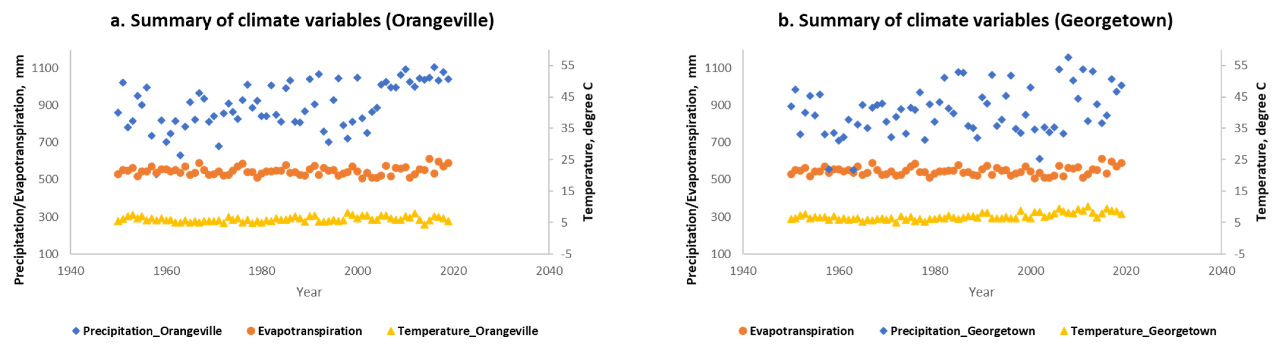
3.2. Spatio-Temporal Changes in Climate Variables

The results of the Mann–Kendall test to detect and attribute the change in mean temperature, total precipitation, and evapotranspiration at the monthly, seasonal, and annual scales at a rural and an urban site for the period of 1950–2019 are shown in Table 3 and Figure 7. Table S1 in the Supplementary Materials provides the τ, p-value, and slope derived from the analysis.
For the rural Orangeville site, the temperature (1950–2019) showed a significant increasing trend for the month of September, as well as the winter, spring, summer, and full year. For the urban Georgetown site, except for January, March, April, and May, the other periods showed a significant increasing trend for temperature. At both stations, the increase in the winter temperature was the main contributor to the increase in the annual temperature. The decadal temperature increase for Orangeville and Georgetown were 0.09 °C and 0.33 °C, respectively. These results concur with those of previous studies [4,8].
Precipitation (1950–2019) showed weak increasing monthly trends except for the month of August (summer month) for both the Orangeville (rural) and Georgetown (urban) sites, and for summer for Georgetown; however, these trends were not significant. The annual precipitation showed a significant increase for both stations. The decadal precipitation change was 33.7 mm for Orangeville (rural) and 16.9 mm for Georgetown (urban).
The annual evapotranspiration (1950–2019) did show an increasing and nonsignificant trend. Compared to other hydrological processes like precipitation, infiltration and runoff, evapotranspiration is a rapid and energy-driven process (rate). It varies regionally and seasonally, as observed in the USA [43]. The lack of a significant trend in evapotranspiration on an annual basis agrees with the results of a recent study reported by [3].
Of the total 85 datasets, 82% showed an increasing trend and 18% showed a decreasing trend. Out of these, 33 datasets had a significant increasing trend and five had a significant decreasing trend. The highest Sen’s slope for temperature and precipitation for the rural Orangeville (0.021 and 0.92) was found for March and April, respectively, and those for the urban Georgetown (0.093 and 0.49) were found for February and April, respectively. Sen’s slope (0.157) for evapotranspiration for the whole watershed was highest for the month of May. These results suggest possible changes in the climate and land use. However, studies relating to temperature, precipitation, and evapotranspiration on a monthly, seasonal, and annual scale for the Great Lakes Basin are few.
The precipitation and evapotranspiration data were analyzed separately in this study because the data were from different sources. This study did not analyze the difference between precipitation (P) and evapotranspiration (E), i.e., the (P-E) trend of the time series data.

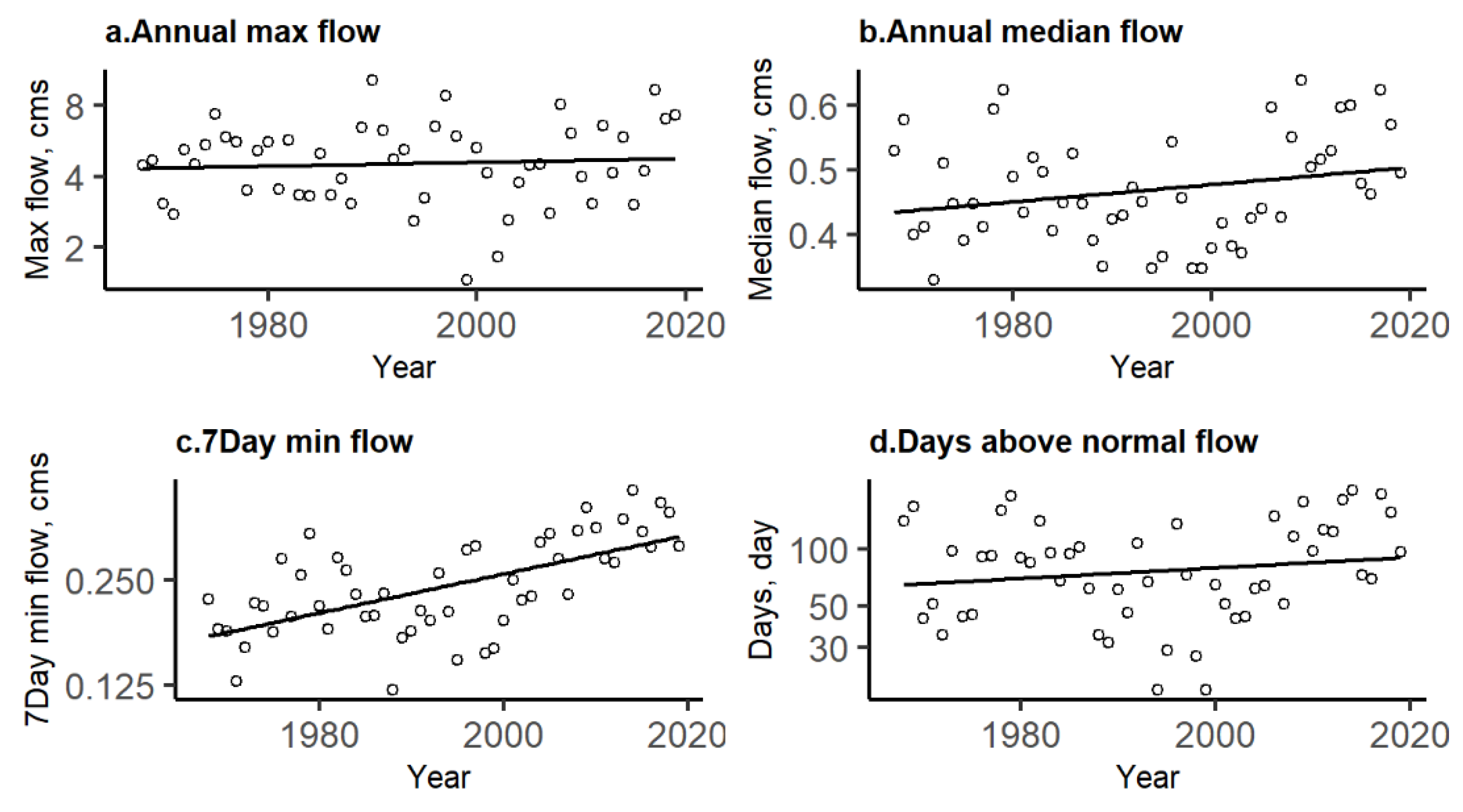
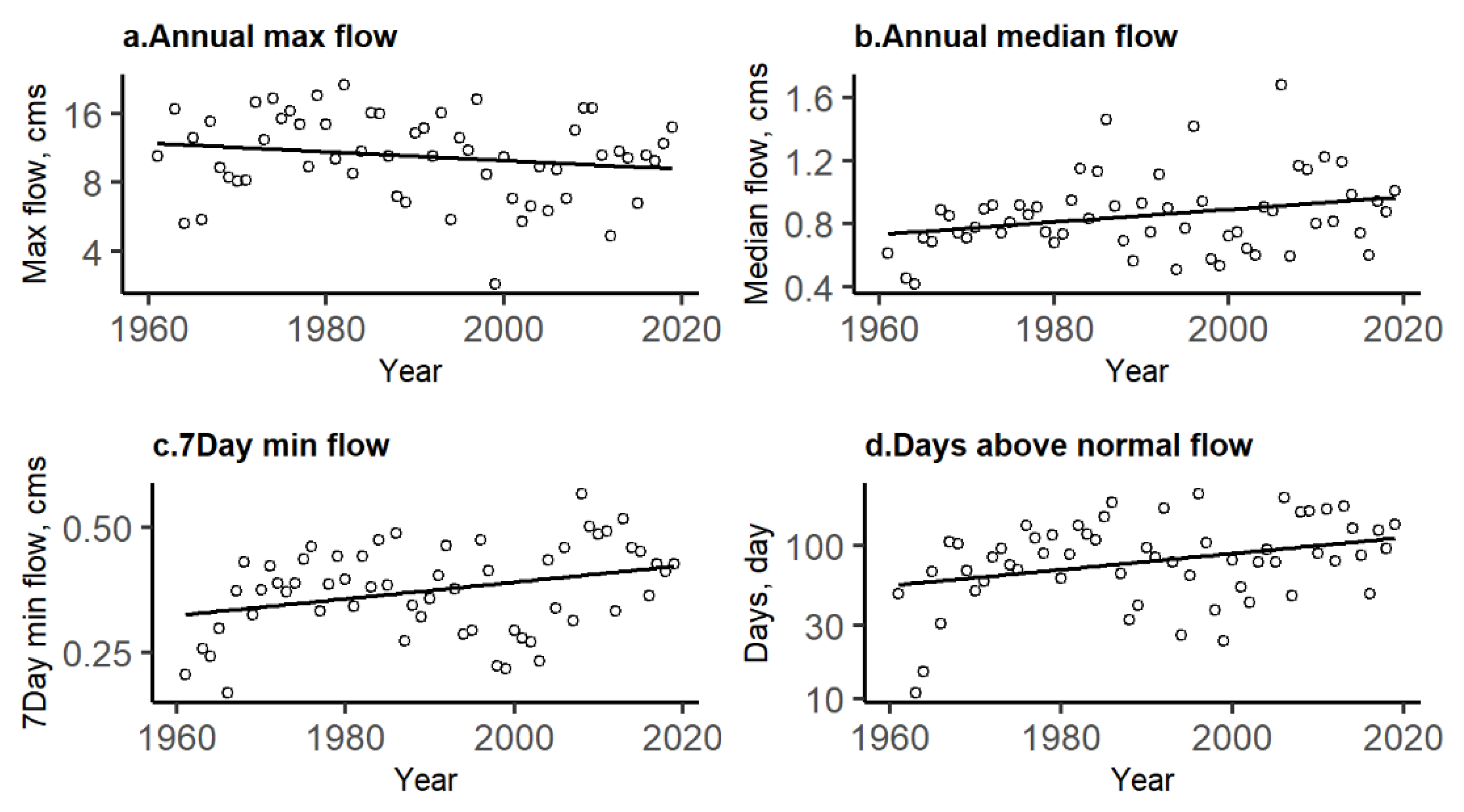
3.3. Spatio-Temporal Changes in the Streamflow

The Period of Record (POR) was divided into sub-periods of 20 years’ worth of data (Table 4). Starting from the headwaters (the upstream location), the gauges at Orangeville, Cataract, Boston Mills, Norval, and Erindale were in the main channel of the Credit River, while those at Erin and West Branch Norval were located on a tributary of the Credit River. The streamflow gauges were divided into two categories based on urbanization and ecoregions: two gauges each (drainage area > 50 km2) were situated in the rural/Lake Simcoe-Rideau ecoregion (Orangeville and Cataract), and another two were situated in the urban/Lake Erie-Lake Ontario ecoregion (Erindale and West Branch Norval). The urban gauge in the tributary channel (West Branch Norval) was selected to negate the cumulative effect of the streamflow from the upstream streamflow.
As an initial screening to detect the streamflow changes, cumulative mass curves were generated for each of the gauges. This assisted in testing any abrupt change in the streamflow due to dams or other structures. All of the gauges showed changes in the streamflow; however, the changes were minor and gradual.
The results of the Mann–Kendall non-parametric (distribution-free) test with Sen’s slope estimator for the streamflow and baseflow at the Cataract, Orangeville, NB Norval and Erindale gauges are presented in Tables S2 and S3 in the Supplementary Materials. The overall picture is represented in Table 5 and Figure 8. An increase in precipitation correlated well with an increase in the streamflow and baseflow. An increase in the spring flow was the main contributor to the significantly increasing trend in the annual flow at Cataract, Orangeville, and WB Norval. In contrast, Erindale showed both positive and negative trends in its streamflow, reflecting the ways in which land-use and climate change are probably compensating for each other’s effects. The decadal streamflow slopes for two gauges, one from a rural (Cataract) and one from an urban (Erindale) gauge, were 0.014 and 0.557 m3 s−1, respectively, while for the baseflow slope values these gauges were 0.02 and 0.431 m3 s−1. Because there are no major hydrotechnical projects in the watershed, the change could be attributable to climate change and land-use change.
Overall, the urban streamflow and baseflow can be concluded to be changing at a faster rate than the rural area due to the build-up of an impervious layer in the watershed, as well as climate change. The increase in the baseflow during winter and summer improves the water quality [44]. Standardized data from Reference Hydrologic Networks’ (RHBN) stream gauges—situated in the UK, USA, and Canada—were used to analyze climate-driven changes in the streamflow; however, it was found that it was difficult to separate the impact of climate change and urbanization [45]. The key issue with this method was that there was a limited number of RHBN gauges (n = 12) on the Canadian side of the Great Lakes Basin, with no RHBN gauge in the Credit River basin. Previous studies [11,12] on the same watershed looked at the projected values from climate models. The study using historic data showed a similar trend, but the data was limited up to 2009 [13].
Out of the total 110 datasets, 78% showed an increasing trend and 28% showed a decreasing trend. Out of these, 30 datasets showed a significant an increasing trend, and one showed a significant decreasing trend. The change was neither dependent on the drainage area nor on the gauge location (main channel/tributary). As there were no major structures or diversions in the watershed, the change was primarily due to climate change and land-cover changes.
Only estimated for the Cataract gauge, the COV value was 1.3 (COV > 1.0; p = 0.03). The slope was –0.304, indicating that every 10 years the COV occurs three days earlier. This is likely driven by warming winter and spring temperatures, and changes in the snow-to-rain ratio [1].
The 10% exceedance and 10:90 exceedance ratios for FDC were estimated, and the data are provided in Table S4 as Supplementary Materials. Although the 10% exceedance did change over the years, it did not show any consistent decrease/increase. In contrast, the annual and winter 10:90 exceedance ratio declined over the years for the rural (Cataract) and urban (WB Norval) gauges, though they did not show a consistent change for the summer and autumn values. The reduction in the ratio during the winter season was likely due to increased temperatures, while for the annual period it was likely due to changes in the streamflow regime. Using the FDC, water flow and yield differences attributed to permanent changes in vegetation cover were observed in a number of paired catchment studies undertaken at different temporal scales [46]. They concluded that it was difficult to generalize the quantitative impact of changes in vegetation on seasonal yield and flow regimes.
In order to assess the changes in the baseflow contribution to the total streamflow, the BFI—a proxy indicator of groundwater discharge and other water storage in the watershed—was determined. The baseflow is considered to be an important parameter for effective water management planning, especially during long dry periods. The BFI (Table S5, Supplementary Materials) changed over time. For the summer and autumn, as well as for the full year, the BFI was >0.5, showing that the watershed is a slow-response watershed with sustained flow and high groundwater storage. This occurs because with warmer winter temperatures the soil freezes and thaws, and there are frequent snowmelt events. In hydrological models for Ontario, the BFI is the variable which is most sensitive to regional low [47] and flood flows [48].
The assumption of stationarity which is necessary for POT flood analysis failed for all gauges and all periods, as the values of the location and shape changed (Table S6, Supplemental Materials). In order to make the analysis physically more meaningful using EVI, the sensitivity of the magnitude of the flood, a normalized value (Q100/Q2), was estimated. Within the five sub-periods (104 years) of the records for the Cataract gauge, the EVI showed periodicity (not monotonic), while at the same time the POR values showed a decreasing trend. As the basin regularly experiences floods in the spring (snowmelt and/or a combination of snowmelt and rain) and summer months, the EVI for the two seasons was compared. For both rural and urban watersheds, the spring EVI was smaller than that in the summer. This indicates that spring floods are more volatile than summer floods. The EVI can also be used as a proxy for event attribution in order to understand the impact of climate change. The amount of precipitation with a certain recurrence interval is projected to increase.
The flood flows (Q2 and Q100) and low flows (7Q2 and 7Q20) for two periods were compared in order to investigate their change (Figure 9 and Figure 10). These values are tied to Ontario regulations: a 100-year flood is the regulatory flood employed in flood plain mapping and development, and a 7Q20 low flow is used as the limiting flow for the abstraction and discharge of water from/to the stream. A 2-year return period is used as an index flood in Ontario regional flood models [48]. These data indicate that the flood flow decreased while the low flow increased from the earlier (up to 1984) to the current period (up to 2019). This was further investigated by looking at the parent (precipitation) data series over the years.
In Ontario, the annual maximum precipitation data is bimodal due to low-likelihood, high-frequency events happening once in three to four years. The number of these outliers of high magnitude increases as the period of record increases. Accordingly, the Intensity, Duration and Frequency (IDF) precipitation values may increase because the extreme outliers (historic events) are never removed. Due to global warming, it is anticipated that the snowmelt will happen earlier, and hence rainfall events that usually occur during April–May are not snowmelt on rainfall events. Because of the compensating effect of the decrease in snow cover, storm events are not producing riverine floods (no outliers); this may also be due to the earlier occurrence of the peak streamflow. Low antecedent soil moisture values and the greater availability of watershed/channel storage capacity are the main physiographic reasons for this effect. Flood flows were studied at the watershed scale [28,29]; however, flood flows and low flows should be studied at a regional scale, rather than on a watershed scale [49,50].
Furthermore, the Cataract gauge, with the longest duration of data, was further investigated for all five sub-periods. The results showed an increase as well as a decrease for the median streamflow, baseflow, and BFI; an increase in the low flow; and a decrease in the flood flow and POT (the magnitude of the flood). This could be due to climate change. The warming of temperatures results in an increase in rainfall and a decrease in snowfall during the winter and early spring periods. This results in reduced flows due to snowmelt.
A preliminary review (starting 1851) was carried out on the land-use change within the watershed. During 1851–1890, the land cover was dominated with forest and wetland. Then, until 1940, watershed development started to convert it to urban and agriculture land use. Then, re-forestation happened until 1954. A summary of the land use for three periods—1956, 1996, 2010, and 2015—is given in Table 6 [24,31]. With the progress of time, land use management practice has changed in a complex way, along with municipal official planning; hence, a detailed study is warranted.

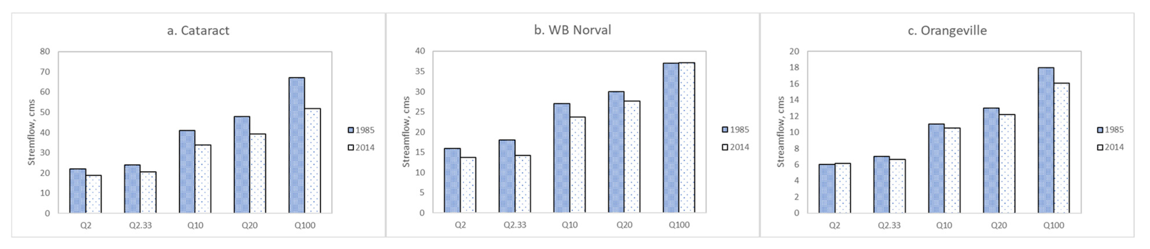
3.4. Spatial Analysis between Rural and Urban Stream Gauges

The initial screening was performed using Pettitt’s test and population growth data for the regions around the Cataract (rural) and West Branch Norval (urban) stream gauges; data for the 1971–2019 period were selected for analysis. Concomitant data for the nearby climate stations (Orangeville and Georgetown) were also selected for the same period for analysis.
The results of the Mann–Kendall trend analysis for the annual and seasonal time series for the mean temperature, total precipitation, evapotranspiration, and median streamflow are shown in Table 7. Details of the statistics (τ, p-value, and slope) of these test results are provided in Table S7 of the Supplementary Materials. Except for the winter (rural) and summer (urban) precipitation, which showed a negative temporal trend, in all other cases (temperature and precipitation) a positive trend was observed. The evapotranspiration within the watershed (as the GLDAS resolution is high) was taken for reference. There were significant changes (increases or decreases) in the evapotranspiration for the spring and autumn seasons. For the rural areas, the median streamflow showed a significant increase for the annual, winter, and spring periods. Out of the total 35 datasets, 86% showed an increasing trend and 14% showed a decreasing trend. Out of these, 12 datasets showed a significant increasing trend, and none showed a significant decreasing trend.
In order to compare the rural and urban sub-watersheds, Sen’s slope of streamflow was normalized with the annual precipitation and temperature. Overall, the annual streamflow increased for all of the gauges. However, the rural (vs. urban) areas were more sensitive to both temperature and precipitation (Figure 11 and Figure 12), perhaps because of the sinusoidal variability in the minimum and maximum temperatures that occurs between the two areas, as suggested by another study [51]. When analyzed for seasonal data in sequence, the winter streamflow showed a decline, whereas, for the same time for other periods, it showed an increasing trend in the rural areas. However, the urban areas were underwater because of the increase in winter flow (snowmelt or precipitation falling as rain); therefore, the spring freshet was reduced. Furthermore, exaggerating the process, lower precipitation during the summer would result in a low streamflow not only during the summer but also into the coming autumn, as the historical data has shown in this study.
The BFI results show that the BFI of the rural areas was, on average, 18% higher than that of the urban areas (Table 8). This proxy parameter for impervious built-up areas shows that an increase in these areas in urban zones reduces the baseflow of the stream. This trend is visible and consistent for the annual analysis. The highest percentage change between the two gauging stations was found during the winter season, i.e., 21.6%. The lowest BFI difference for these stations was found during the spring season, i.e., 12.5%.
The analysis of the surface Runoff Coefficient (RC) for the rural and urban gauges, Cataract and WB Norval, respectively, is shown in Figure 13. The annual RC for the urban gauge area was 19.3% higher than that for the rural area gauge, and this was due to the higher percentage of impervious areas in the urban zone. A similar trend was observed for spring, summer, and autumn. However, the difference of the RC was the lowest (5.8%) in the summer (Figure 13). In addition, the analysis of the RC for various periods (C, D, and E) also shows the greater contribution of surface runoff from urban areas compared to rural areas. This indicates that climate change and urbanization affect the changes in the streamflow. However, even though different methods have been tried, there is no feasible method to separate the impact of climate change and that of land-use change [23].

4. Conclusions

The goal of the present study was to evaluate the impact of climate change, land cover, and land-use change on the streamflow in the rapidly urbanizing Credit River watershed, which drains into Lake Ontario at Port Credit (Ontario, Canada). For some of the gauging stations, streamflow data were available for a period of over 100 years. The non-parametric Mann–Kendall test with Sen’s Slope estimator method was used to detect changes in the climate variables (temperature, precipitation, and evapotranspiration) and streamflow characteristics (median annual streamflow, baseflow, and COV). Other streamflow characteristics that were studied tested the stationarity of the peak over the threshold streamflow using EVT, duration curves and their derivatives, BFI, and runoff coefficient. A total of 230 datasets were tested for their trends; of these, 80% and 20% increasing and decreasing trends, respectively, were obtained. Of the total, significant trends (<0.05%) of 32% and 2% increasing and decreasing trends were found, respectively.
  • The analysis of the annual mean temperature and precipitation showed significant trends; however, evapotranspiration showed no such trends. The rural gauges tended to show increasing monthly and seasonal trends for precipitation, whereas the urban gauges tended to show increasing trends for temperature. Of the total 85 datasets, 82% of the datasets showed an increasing trend and 18% showed a decreasing trend. Out of these, 33 datasets showed a significant increasing trend and five datasets showed a significant decreasing trend. Over a ten-year period, the COV shifted three days earlier, showing that the fraction of streamflow happening each month was changing, driven by warming winter temperatures.
  • Both the streamflow and baseflow showed trends. Out of the total 110 datasets, 78% of the datasets showed an increasing trend and 28% showed a decreasing trend. Out of these, 30 datasets showed a significant increasing trend, and one showed a significant decreasing trend. The FDC derivative—10% exceedance, which was used to detect the lateral shifts in the streamflow—did not show any consistent increase/decrease in values; however, the 10:90 exceedance ratio declined over the years but did not show any consistent change in its summer or autumn values.
  • The BFI index varied during the latter two periods (Periods D and E). In general, if BFI > 0.5, the watershed could be deemed to have a slow response. The stationarity test was failed for the POT analysis. Though the magnitude of the likelihood of a flood changed, this change showed no clear pattern. At the same time, the flood and low flow frequencies decreased and increased, respectively. This change in the latter period, highlighting the fact that the annual peak declined over the years, at the same time as the annual seven-day minimum increased. The runoff coefficient showed a consistent behavior for the winter, spring, and autumn periods, where evapotranspiration was not a dominating factor. This implies that land use has played a significant role in the watershed’s hydrology for urban regions.
  • A spatial analysis of both rural and urban gauges was used to attribute changes in streamflow to temperature and/or precipitation, which showed that rural zones were more sensitive to temperature and precipitation than urban zones. The same was the case for BFI. Out of the total 35 datasets, 86% showed an increasing trend and 14% showed a decreasing trend. Out of these, 12 datasets showed a significant increasing trend, and none showed a significant decreasing trend.
Overall, the findings from this study highlight the annual, monthly, and seasonal changes in the temperature, precipitation, and streamflow in a rapidly urbanizing watershed in the Lake Ontario Basin. However, it was difficult to clearly quantify the changes in the streamflow over the decade which were attributable to population growth and the expansion of urban areas. The study further revealed that more detailed, continuous, spatio-temporal land-cover and land-use data regarding the expansion of urban areas are needed in order to better quantify the impact of urbanization on the streamflow, as changes in the streamflow associated with changes in land use would potentially impact the water quality and water levels in the Great lakes. Therefore, a more detailed investigation of the impact of urbanization on the hydrology and water quality for the watersheds in the Great Lakes region is recommended. In addition, watershed modelling methods with detailed monitoring data should be employed in order to segregate the impact of land cover and land-use changes from the impact of climate change on the streamflow and hydrology of the watershed.

Supplementary Materials

The following are available online at www.mdpi.com/article/10.3390/atmos13020225/s1, Table S1: Summary of the trend analysis for the temperature, precipitation, and evapotranspiration variables annually, seasonally, and monthly, Table S2: Summary of the trend analysis of the streamflow. Period A, 1920–1939; Period B, 1940–1959; Period C, 1960–1979; Period D, 1980–1999; Period E, 2000–2019, Table S3: Summary of the trend analysis of the baseflow. Period A, 1920–1939; Period B, 1940–1959; Period C, 1960–1979; Period D, 1980–1999; Period E, 2000–2019, Table S4: Summary of the FDC 10% exceedance and 10:90% exceedance ratio. Period A, 1920–1939; Period B, 1940–1959; Period C, 1960–1979; Period D, 1980–1999; Period E, 2000–2019, Table S5: Summary of the BFI for different periods. Period A, 1920–1939; Period B, 1940–1959; Period C, 1960–1979; Period D, 1980–1999; Period E, 2000–2019, Table S6: Summary of the POT analysis parameters and return level for 2 years, 10 years, 20 years, 100 years, and its derivative. Period A, 1920–1939; Period B, 1940–1959; Period C, 1960–1979; Period D, 1980–1999; Period E, 2000–2019, Table S7: Summary of the trend analysis for the period 1971–2019, Table S8: Summary of the trend analysis for the period 1971–2019.

Author Contributions

All of the analysis of the data, and the preparation of the manuscripts were primarily completed by E.P., under the supervision of R.P.R., P.K.G. and S.I.A. Conceptualization, E.P., R.P.R., P.K.G. and S.I.A.; methodology, E.P., R.P.R., P.K.G. and S.I.A., formal analysis, E.P.; investigation, E.P., R.P.R., P.K.G. and S.I.A.; resources, E.P., R.P.R., P.K.G. and S.I.A.; data curation, E.P.; writing—original draft preparation, E.P., R.P.R., P.K.G. and S.I.A..; writing—review and editing, E.P., R.P.R., P.K.G. and S.I.A.; visualization, E.P.; supervision, R.P.R.; project administration, R.P.R. All authors have read and agreed to the published version of the manuscript.

Funding

This research received no external funding.

Institutional Review Board Statement

Not applicable.

Informed Consent Statement

Not applicable.

Data Availability Statement

The data were taken from the publicly available sources.

Conflicts of Interest

The authors declare no conflict of interest.

References

  1. Bush, E.; Lemmen, D.S. Canada’s Changing Climate Report; Government of Canada: Ottawa, ON, Canada, 2019; p. 444. Available online: https://changingclimate.ca/site/assets/uploads/sites/2/2020/06/CCCR_FULLREPORT-EN-FINAL.pdf (accessed on 22 October 2021).
  2. Reidmiller, D.R.; Avery, C.W.; Easterling, D.R.; Kunkel, K.E.; Lewis, K.L.M.; Maycock, T.K.; Stewart, B.C. USGCRP Impacts, Risks, and Adaptation in the United States: Fourth National Climate Assessment, Volume II; U.S. Global Change Research Program: Washington, DC, USA, 2018; p. 1515. [CrossRef]
  3. Mailhot, E.; Music, B.; Nadeau, D.F.; Frigon, A.; Turcotte, R. Assessment of the Laurentian Great Lakes’ hydrological conditions in a changing climate. Clim. Chang. 2019, 157, 243–259. [Google Scholar] [CrossRef] [Green Version]
  4. Houghton, E.; Meiro Filho, L.G.; Callander, B.A.; Harris, N.; Kattenburg, A.; Maskell, K. Climate Change 1995: The Science of Climate Change: Contribution of Working Group I to the Second Assessment Report of the Intergovernmental Panel on Climate Change; Cambridge University Press: Cambridge, UK, 1996; Available online: https://digitallibrary.un.org/record/223181?ln=en (accessed on 22 October 2021).
  5. Egerton, F.N. History of Ecological Sciences, Part 60: American Great Lakes before. Bull. Ecol. Soc. Am. 2018, 99, 77–136. [Google Scholar] [CrossRef] [Green Version]
  6. Scott, R.W.; Huff, F.A. Impacts of the Great Lakes on Regional Climate Conditions. J. Great Lakes Res. 1996, 22, 845–863. [Google Scholar] [CrossRef]
  7. Wuebbles, D.; Cardinale, B.; Cherkauer, K.; Davidson-Arnott, R.; Hellmann, J.J.; Infante, D.; Johnson, L.; de Loë, R.; Lofgren, B.; Packman, A.; et al. An Assessment of the Impacts of Climate Change on the Great Lakes; The Environmental Law & Policy Center and the Chicago Council on Global Affairs: Chicago, IL, USA, 2019. Available online: https://www.climatehubs.usda.gov/sites/default/files/Great-Lakes-Climate-Change-Report.pdf (accessed on 22 October 2021).
  8. Ahmed, S.I.; Rudra, R.; Dickinson, T.; Ahmed, M. Trend and Periodicity of Temperature Time Series in Ontario. Am. J. Clim. Chang. 2014, 3, 272–288. [Google Scholar] [CrossRef] [Green Version]
  9. Adamowski, K.; Bougadis, J. Detection of trends in annual extreme rainfall. Hydrol. Process. 2003, 17, 3547–3560. [Google Scholar] [CrossRef]
  10. Rudra, R.P.; Dickinson, W.T.; Ahmed, S.I.; Patel, P.; Zhou, J.; Gharabaghi, B.; Khan, A.A. Changes in Rainfall Extremes in Ontario. Int. J. Environ. Res. 2015, 9, 1117–1126. [Google Scholar] [CrossRef]
  11. Champagne, O.; Arain, M.A.; Coulibaly, P. Atmospheric circulation amplifies shift of winter streamflow in southern Ontario. J. Hydrol. 2019, 578, 124051. [Google Scholar] [CrossRef]
  12. Champagne, O.; Arain, M.A.; Leduc, M.; Coulibaly, P.; McKenzie, S. Future shift in winter streamflow modulated by the internal variability of climate in southern Ontario. Hydrol. Earth Syst. Sci. 2020, 24, 3077–3096. [Google Scholar] [CrossRef]
  13. Singh, A.; Dougherty, J.; Zimmer, C.; Kinkead, J.; Hulley, M.; Doherty, C. Assessing Trends in Temperature, Precipitation and Streamflow due to Climate Change in Credit River Watershed. In Proceedings of the CCTC 2009: 2nd Climate Change Technology Conference, Hamilton, ON, Canada, 12–15 May 2009. [Google Scholar]
  14. Taylor, C.H.; Roth, D.M. Effects of suburban construction on runoff contributing zones in a small southern Ontario drainage basin. Hydrol. Sci. Bull. 1979, 24, 289–301. [Google Scholar] [CrossRef] [Green Version]
  15. Ko, C.; Cheng, Q. GIS spatial modeling of river flow and precipitation in the Oak Ridges Moraine area, Ontario. Comput. Geosci. 2004, 30, 379–389. [Google Scholar] [CrossRef]
  16. Morgan, A.; Branfireun, B.; Csillag, F. An Evaluation of the Contributions of Urbanization and Climatic Change to Runoff Characteristics in the Laurel Creek Watershed, Ontario. Can. Water Resour. J. 2004, 29, 171–182. [Google Scholar] [CrossRef] [Green Version]
  17. Muñoz, L.A.; Olivera, F.; Giglio, M.; Berke, P. The impact of urbanization on the streamflows and the 100-year floodplain extent of the Sims Bayou in Houston, Texas. Int. J. River Basin Manag. 2017, 16, 61–69. [Google Scholar] [CrossRef]
  18. Song, X.; Zhang, J.; Agha Kouchak, A.; Roy, S.S.; Xuan, Y.; Wang, G.; He, R.; Wang, X.; Liu, C. Rapid urbanization and changes in spatiotemporal characteristics of precipitation in Beijing metropolitan area. J. Geophys. Res. Atmos. 2014, 119, 11–250. [Google Scholar] [CrossRef] [Green Version]
  19. Whitney, J.W.; Glancy, P.A.; Buckingham, S.E.; Ehrenberg, A.C. Effects of rapid urbanization on streamflow, erosion, and sedimentation in a desert stream in the American Southwest. Anthropocene 2015, 10, 29–42. [Google Scholar] [CrossRef]
  20. Cunderlik, J.M.; Simonovic, S.P. Hydrological extremes in a southwestern Ontario river basin under future climate conditions/Extrêmes hydrologiques dans un basin versant du sud-ouest de l’Ontario sous conditions climatiques futures. Hydrol. Sci. J. 2005, 50, 1–654. [Google Scholar] [CrossRef]
  21. Konrad, C.P.; Booth, D.; Burges, S.J. Effects of urban development in the Puget Lowland, Washington, on interannual streamflow patterns: Consequences for channel form and streambed disturbance. Water Resour. Res. 2005, 41, 07009. [Google Scholar] [CrossRef]
  22. Martin, E.H.; Kelleher, C.; Wagener, T. Has urbanization changed ecological streamflow characteristics in Maine (USA)? Hydrol. Sci. J. 2012, 57, 1337–1354. [Google Scholar] [CrossRef] [Green Version]
  23. Zeng, F.; Ma, M.-G.; Di, D.-R.; Shi, W.-Y. Separating the Impacts of Climate Change and Human Activities on Runoff: A Review of Method and Application. Water 2020, 12, 2201. [Google Scholar] [CrossRef]
  24. CVC (Credit Valley Conservation). Strategic Plan, Final Version. 2007. Available online: https://cvc.ca/wp-content/uploads/2011/10/CVC-Strategic-Plan06.pdf (accessed on 22 October 2021).
  25. OMNRF (Ontario Ministry of Natural Resources and Forestry (MNRF). Infilled Climate Data. 2007. Available online: https://data.ontario.ca/dataset/in-filled-climate-data (accessed on 22 October 2021).
  26. NASA Earth Data. Giovanni Ver. 4. Available online: https://giovanni.gsfc.nasa.gov/giovanni/ (accessed on 22 October 2021).
  27. Ontario Ministry of Northern Development, Mines, Natural Resources and Forestry (MNRF). Ontario Flow Assesment Tool (OFAT). 2012. Available online: http://www.gisapplication.lrc.gov.on.ca/webapps/OFAT/Viewer/Viewer.html?lang=en-US (accessed on 22 October 2021).
  28. Trudeau, M.; Richardson, M. Change in event-scale hydrologic response in two urbanizing watersheds of the Great Lakes St Lawrence Basin 1969–2010. J. Hydrol. 2015, 523, 650–662. [Google Scholar] [CrossRef]
  29. Trudeau, M.; Richardson, M. Empirical assessment of effects of urbanization on event flow hydrology in watersheds of Canada’s Great Lakes-St Lawrence basin. J. Hydrol. 2016, 541, 1456–1474. [Google Scholar] [CrossRef]
  30. Whitfield, P.H.; Cannon, A.J. Recent Variations in Climate and Hydrology in Canada. Can. Water Resour. J. Rev. 2000, 25, 19–65. [Google Scholar] [CrossRef]
  31. Government of Canada, Natural Resources Canada, Canada Centre for Remote Sensing. Landsat Satellite Data, Land Cover of Canada-Cartographic Product Collection. Available online: https://open.canada.ca/data/en/dataset/11990a35-912e-4002-b197-d57dd88836d7 (accessed on 27 December 2021).
  32. Ashraf, M.S.; Ahmad, I.; Khan, N.M.; Zhang, F.; Bilal, A.; Guo, J. Streamflow Variations in Monthly, Seasonal, Annual and Extreme Values Using Mann-Kendall, Spearmen’s Rho and Innovative Trend Analysis. Water Resour. Manag. 2021, 35, 243–261. [Google Scholar] [CrossRef]
  33. Chen, Y.; Guan, Y.; Shao, G.; Zhang, D. Investigating Trends in Streamflow and Precipitation in Huangfuchuan Basin with Wavelet Analysis and the Mann-Kendall Test. Water 2016, 8, 77. [Google Scholar] [CrossRef] [Green Version]
  34. Norton, P.A.; Driscoll, D.G.; Carter, J.M. Climate, Streamflow, and Lake-Level Trends in the Great Lakes Basin of the United States and Canada, Water Years 1960–2015; US Geological Survey: Reston, VA, USA, 2019.
  35. Yue, S.; Pilon, P.; Phinney, B. Canadian streamflow trend detection: Impacts of serial and cross-correlation. Hydrol. Sci. J. 2003, 48, 51–63. [Google Scholar] [CrossRef]
  36. Yue, S.; Pilon, P.; Cavadias, G. Power of the Mann–Kendall and Spearman’s rho tests for detecting monotonic trends in hydrological series. J. Hydrol. 2002, 259, 254–271. [Google Scholar] [CrossRef]
  37. Yulianti, J.S.; Burn, D.H. Investigating Links Between Climatic Warming and Low Streamflow In The Prairies Region Of Canada. Can. Water Resour. J. 1998, 23, 45–60. [Google Scholar] [CrossRef]
  38. Zhang, X.; Harvey, K.D.; Hogg, W.D.; Yuzyk, T.R. Trends in Canadian streamflow. Water Resour. Res. 2001, 37, 987–998. [Google Scholar] [CrossRef]
  39. Nathan, R.J.; McMahon, T.A. Evaluation of automated techniques for base flow and recession analyses. Water Resour. Res. 1990, 26, 1465–1473. [Google Scholar] [CrossRef]
  40. Dickens, C.; Smakhtin, V.; Biancalani, R.; Villholth KEriyagama, N.; Marinelli, M. Incorporating Environmental Flows into “Water Stress” Indicator 6.4. Guidelines for a Minimum Standard Method for Global Reporting; FAO: Rome, Italy, 2019; Available online: https://www.fao.org/3/ca3097en/CA3097EN.pdf (accessed on 22 October 2021).
  41. Ganguly, A.R.; Steinhaeuser, K. Data Mining for Climate Change and Impacts. In Proceedings of the 2008 IEEE International Conference on Data Mining Workshops, Institute of Electrical and Electronics Engineers (IEEE), Pisa, Italy, 15–19 December 2008; pp. 385–394. [Google Scholar]
  42. Metcalfe, R.A.; Schmidt, B. Streamflow Analysis and Assessment Software (SAAS) (V4.1). Available online: http://people.trentu.ca/rmetcalfe/SAAS.html (accessed on 22 October 2021).
  43. Hanson, R.L. Evapotranspiration and Droughts, Water-Supply Paper. In National Water Summary 1988–89—Hydrologic Events and Floods and Droughts; Paulson, R.W., Chase, E.B., Roberts, R.S., Moody, D.W., Eds.; U.S. Geological Survey: Reston, VA, USA, 1991. Available online: https://geochange.er.usgs.gov/sw/changes/natural/et/ (accessed on 22 October 2021).
  44. Novotny, E.V.; Stefan, H.G. Stream flow in Minnesota: Indicator of climate change. J. Hydrol. 2007, 334, 319–333. [Google Scholar] [CrossRef]
  45. Burn, D.H.; Hannaford, J.; Hodgkins, G.A.; Whitfield, P.H.; Thorne, R.; Marsh, T. Reference hydrologic networks II. Using reference hydrologic networks to assess climate-driven changes in streamflow. Hydrol. Sci. J. 2012, 57, 1580–1593. [Google Scholar] [CrossRef] [Green Version]
  46. Brown, A.E.; Zhang, L.; McMahon, T.A.; Western, A.W.; Vertessy, R.A. A review of paired catchment studies for determining changes in water yield resulting from alterations in vegetation. J. Hydrol. 2005, 310, 28–61. [Google Scholar] [CrossRef]
  47. Ontario Ministry of the Environment (MOE). Regionalization of Low Flow Characteristics for Various Regions in Ontario; Ministry of Environment (MOE): ON, Canada, 2020.
  48. Moin, S.; Shaw, M. Canada/Ontario Flood Damage Reduction Program–Regional Flood Frequency Analysis for Ontario Streams; Environment Canada: ON, Canada, 1985; Volumes 1–3.
  49. Katz, R.; Parlange, M.; Naveau, P. Statistics of extremes in hydrology. Adv. Water Resour. 2002, 25, 1287–1304. [Google Scholar] [CrossRef] [Green Version]
  50. Mahmood, R.; Pielke, R.A.; Hubbard, K.; Niyogi, D.; Bonan, G.; Lawrence, P.; McNider, R.; McAlpine, C.; Etter, A.; Gameda, S.; et al. Impacts of Land Use/Land Cover Change on Climate and Future Research Priorities. Bull. Am. Meteorol. Soc. 2010, 91, 37–46. [Google Scholar] [CrossRef]
  51. Evan, A.; Eisenman, I. A mechanism for regional variations in snowpack melt under rising temperature. Nat. Clim. Chang. 2021, 11, 326–330. [Google Scholar] [CrossRef]
Figure 1. Credit River watershed with the locations of the streamflow and climate stations. The number indicates the drainage area (km2) and elevation (m).
Atmosphere 13 00225 g001
Figure 2. Annual mean temperature, total annual precipitation, and evapotranspiration (1950–2019) of the rural (a) Orangeville and urban (b) Georgetown sites.
Atmosphere 13 00225 g002
Figure 3. Streamflow regime of the Cataract (rural) gauge located in the main channel. (a) Annual max flow, (b) Annual median flow, (c) 7-day min flow, (d) Days above normal flow.
Atmosphere 13 00225 g003
Figure 4. Streamflow regime of the Orangeville (rural) gauge located in the main channel. (a) Annual max flow, (b) Annual median flow, (c) 7-day min flow, (d) Days above normal flow.
Atmosphere 13 00225 g004
Figure 5. Streamflow regime of the WB Norval (urban) gauge located on a tributary. (a) Annual max flow, (b) Annual median flow, (c) 7-day min flow, (d) Days above normal flow.
Atmosphere 13 00225 g005
Figure 6. Streamflow regime of the Erindale (urban) gauge located in the main channel. (a) Annual max flow, (b) Annual median flow, (c) 7-day min flow, (d) Days above normal flow.
Atmosphere 13 00225 g006
Figure 7. Sen’s slope values for precipitation and temperature for (a) Orangeville and (b) Georgetown for 12 months (1 to 12), winter (13), spring (14), summer (15), and autumn (16), and annually (17). The number in the bracket shows the time period in the x-axis.
Atmosphere 13 00225 g007
Figure 8. Sen’s slope summary of the (a) streamflow and (b) baseflow.
Atmosphere 13 00225 g008
Figure 9. Comparison of the flood flows for the return periods Q2, Q2.33, Q10, Q50 and Q100 from 1985 to 2014 for two rural stream gauges (c) Orangeville and (a) Cataract and one urban gauge (b) WB Norval. The graph shows a decrease in the return level in 2014.
Atmosphere 13 00225 g009
Figure 10. Comparison of the low flows for the return periods 7Q2 and 7Q20 from 1995 to 2019 for two rural gauges (c) Orangeville and (a) Cataract and one urban gauge (b) WB Norval. The graph shows an increase in the return level in 2019.
Atmosphere 13 00225 g010
Figure 11. Cataract and WB Norval annual and seasonal streamflow changes normalized (for comparison) with the temperature for the period 1971–2019. The Cataract (rural) gauge shows a greater increase in streamflow.
Atmosphere 13 00225 g011
Figure 12. Cataract and WB Norval annual and seasonal streamflow changes normalized with the precipitation for the period 1971–2019. The change for the urban gauge is negative.
Atmosphere 13 00225 g012
Figure 13. Runoff coefficients of the rural and urban sections of the watershed. (a) Period of record, (b) Sub-periods.
Atmosphere 13 00225 g013
Table 1. Concomitant streamflow and climate gauges selected for the present study.
Streamflow GaugeClimate GaugeStreamflow GaugeClimate Gauge
RuralUrban
OrangevilleOrangevilleWB NorvalGeorgetown
CataractOrangevilleErindaleGeorgetown
Table 2. Climate and streamflow matrix used for the analysis.
AnalysisParameters
MeteorologicalHydrological
TemperaturePrecipitationEvapotranspirationStreamflowBaseflowFlow Duration
Curve
Annual/seasonal/monthly trend
Annual/seasonal/sub-period trend
Annual/seasonal/sub-period peak over threshold
Annual flood frequency
Annual low flow frequency
Annual/seasonal/sub-period runoff coefficient
Centre of volume trend
Annual/seasonal/sub-period baseflow index
Annual/seasonal/sub-period 10% exceedance
Annual/seasonal/sub-period 10:90 exceedance
Table 3. Results of the monthly, seasonal, and annual trend analysis of the temperature, precipitation, and evapotranspiration for the period 1950–2019.
TimeTemperaturePrecipitationEvapotranspiration
OrangevilleGeorgetownOrangevilleGeorgetownWatershed Average
January↑↑↓↓
February↑↑↑↑↓↓
March
April
May↑↑↑↑↑↑
June↑↑↑↑
July↑↑
August↑↑
September↑↑↑↑
October↑↑↑↑
November↑↑↑↑↓↓
December↑↑↑↑↓↓
Winter↑↑↑↑↑↑↓↓
Spring↑↑↑↑↑↑↑↑
Summer↑↑↑↑
Autumn↑↑↑↑
Annual↑↑↑↑↑↑↑↑
↓ Increasing trend, ↑ decreasing trend, ↑↑ significant (<0.05%) increasing trend, ↓↓ significant (<0.05%) decreasing trend.
Table 4. Period of record and the sub-period chosen for each of the stream gauges.
GaugeDrainage Area (km2)Period of Record
(POR)
Chosen Sub-Period
1920–1939
(A)
1940–1959
(B)
1960–1979
(C)
1980–1999
(D)
2000–2019
(E)
Cataract (Rural)2091916–2019
Erindale (Urban)7951949–1993
West Branch Norval (Urban)1311961–2019
Orangeville (Rural)60.61968–2019
Boston Mills (Rural)4151983–2019
Erin (Rural)32.31984–2019
Norval (Urban)6451989–2019
Table 5. Significant (up/down arrow) and non-significant (horizontal arrow) temporal trends in the streamflow and baseflow. Period A, 1920–1939; Period B, 1940–1959; Period C, 1960–1979; Period D, 1980–1999; Period E, 2000–2019.
Streamflow TrendBaseflow Trend
Period
ABCDEABCDE
Annual
Cataract↑↑↑↑
Orangeville ↑↑ ↑↑
Erindale ↑↑ ↑↑
WB Norval ↑↑ ↑↑
Winter
Cataract↑↑
Orangeville ↑↑ ↑↑
Erindale ↑↑
WB Norval
Spring
Cataract↑↑↑↑
Orangeville ↑↑ ↑↑
Erindale ↑↑
WB Norval ↑↑ ↑↑
Summer
Cataract↑↑↑↑↑↑
Orangeville ↑↑ ↑↑
Erindale ↑↑
WB Norval
Autumn
Cataract↑↑↑↑
Orangeville ↓↓
Erindale ↑↑
WB Norval ↑↑ ↑↑
↓ Decreasing trend, ↑ increasing trend, ↑↑ significant (<0.05%) increasing trend, ↓↓ significant (<0.05%) decreasing trend.
Table 6. Table showing the land cover percentage for the years 1956 (published data [24]), 1996 [24] (published data), 2010 (Landsat satellite data) and 2015 (Landsat satellite data) [31].
Land UsePercentage Area
1956199620102015
Natural area16.626.528.528.6
Agricultural 80.445.74444.1
Urban/settled area322.722.922.8
OtherN/A1.54.64.5
Table 7. Summary of the trend analysis for the urban and rural stations for the period 1971–2019.
Time PeriodTrending Parameter
MeteorologicalHydrological
TemperaturePrecipitationEvapotranspirationStreamflow
OrangevilleGeorgetownOrangevilleGeorgetownWatershed AverageCataractWB Norval
Annual↑↑↑↑↑↑
Winter↑↑↑↑↑↑
Spring↑↑↑↑↑↑
Summer↑↑↑↑
Autumn↑↑
↓ Decreasing trend, ↑ increasing trend, ↑↑ significant (<0.05%) increasing trend.
Table 8. Summary of the seasonal and annual baseflow index (rural and urban) for the period 1971–2019.
PeriodCataractWB Norval% Change in BFI
Annual0.6750.54918.7
Winter0.6210.48721.6
Spring0.6320.55312.5
Summer0.7610.62917.3
Autumn0.7430.59220.3
Publisher’s Note: MDPI stays neutral with regard to jurisdictional claims in published maps and institutional affiliations.

