Abstract
In coastal areas of southeastern China, multiple flood drivers such as river flow, precipitation and coastal water level can lead to compound flooding which is often much greater than flooding simulated by one flood driver in isolation. Bivariate probability distributions accounting for compound flooding from river discharge and sea level were constructed based on MvCAT (Multivariate Copula Analysis Toolbox) combined with goodness of fit tests in 15 coastal-estuarine regions of Southeastern China. Flood typing-based bivariate probability distributions considering multiple flood-generating mechanisms were also built. Our results indicated that the performance of flood typing-based bivariate distribution was not significantly better than the bivariate probability distribution in coastal-estuarine regions based on the Mann–Whitney U test; the compounding effects of river discharge and sea level had limited impact on bivariate return periods, but had greater impact on coastal flooding risk in terms of design values. Ignoring compounding effects of river discharge and sea level leads to significant underestimation of design values. The results suggest that the compounding effect of river discharge and sea level should be considered when calculating design values in coastal flood risk assessment.
1. Introduction
Coastal flooding in the context of sea-level rise and more intense tropical cyclone activities is one of the most significant natural hazards in coastal-estuarine regions over the globe [1,2,3]. Coastal flooding can be termed as compound events, involving the co-occurrence of multiple flood drivers such as river flow, precipitation and coastal water level [4,5,6]. Flooding in coastal-estuarine regions are compound events determined by the interplay between riverine flooding and storm surges [7,8]. In the coastal-estuarine region, coastal cities are widely distributed because the flat terrain, accessible transportation and adequate water resources provide convenient conditions for urban human settlements [9]. As those coastal cities have experienced much higher economic growth than the inner cities, together with higher population density, coastal flood damages in coastal-estuarine regions are expected to increase significantly [10,11,12]. Therefore, reliable flood risk estimate is demanded in coastal-estuarine regions [13]. Besides, in practical applications, coastal and off-shore structures may suffer from severe damages because of the occurrence of high fluvial flooding and high sea level. In turn, the lack of knowledge concerning their joint statistics may severely limit the effectiveness of coastal, port and offshore structures protection, and can lead to expensive and inappropriate decisions. The coastal flood risk analysis provides new insights to policy makers and impose very stringent regulations on the design of hydrological coastal and off-shore engineering structures.
Flood risk estimate is traditionally based on univariate flood frequency analysis, i.e., fitting distribution functions to ordered sequences of observed flood peaks (often annual maximum daily flow) and applied for assessment of riverine flood hazard [14]. Given the dependence among the flood drivers (e.g., storm tide and river flow), univariate flood frequency analysis may lead to severe over or underestimation of flood risk [15,16]. Hence, conventional univariate analysis cannot be applied for flood risk assessment in coastal-estuarine regions. This points to the potential importance of multivariate flood frequency analysis in estimating coastal flooding risk. In regard to the coastal flooding risk approach, the possibility of joint occurrence of storm surge and riverine floods based on observed data has been demonstrated, and, hence, bivariate flood frequency analysis has been explored along in coastal areas such as British, Australian, US, China coasts and Dutch coasts [8,17,18,19]. Moreover, the importance of considering the dependence between river discharge and storm surge in the flood risk has been demonstrated by projected changes in compound flood hazard from riverine and coastal floods [20], global scale assessment of the joint influence of riverine and coastal drivers of flooding in deltas [21,22]. In terms of coastal flood risk, many studies also emphasized the dependence between precipitation and storm surge [23,24,25]. Along the coasts of China, previous studies put more attention on the compound effects of storm surge and rainfall on coastal flooding risk at urban scale [19,26,27], but few considered the dependence between river discharge and storm surge in the flood risk analysis. In terms of methods of flood risk estimation, a number of multivariate statistical models are available to represent the dependence between extremes between river discharge and storm surge [28,29,30]. The most common method is copula. Copula has the advantage of model the dependence structure independently of the marginal distributions compared to standard classical bivariate distribution models [31,32,33]. Copula is widely implemented in analyzing dependence structure of multiple variables in compound extreme events analysis [8,34,35,36].
Either univariate or bivariate flood frequency analysis in general are based on the i.i.d. assumption: data points need to be random variables, independent and identically distributed and data should be originated from the same (identical) underlying distribution [30]. Previous studies showed that flood frequency analysis in locations where a mix of flood-generating mechanisms such as frontal storms, localized thunderstorms and rain-on-snow events exist has been shown to invalidate the i.i.d. assumption [37,38]. To solve this problem, a mixed distribution model was proposed by Singh et al. [39] and then has been widely used for univariate flood frequency analysis [40,41,42]. Moreover, De Niel et al. [43] verified that mixed distribution model with prior separation of flood types is more accurate than conventional distribution model for univariate flood frequency analysis. However, few researches considered the impacts of mixed flood-generating mechanisms on the estimated flood hazard for bivariate flood frequency analysis. In the coastal-estuarine region of southeastern China, riverine floods are mainly generated by frontal (local monsoon) rainfall and western Pacific tropical-cyclone-induced rainfall [44] and the hydrographic characteristics of these two flood types has been demonstrated to be different [45]. Hence, it is necessary to analyze the impact of mixed flood-generating mechanisms on coastal flood risk in the coastal-estuarine region of southeastern China.
The objectives of this study are as follows: (i) to analyze the impact of mixed flood-generating mechanisms on bivariate probability distribution; (ii) to evaluate the compounding effect of river discharge and sea level on coastal flood risk. This study is organized as follows. Section 2 presents the study area, data and the methods used to establish a bivariate probability distribution and model a flood typing-based bivariate distribution. Section 3 describes the compound effects of storm surge and rainfall on coastal flooding risk through the calculated bivariate return period and bivariate design values. The impact of mixed flood-generating mechanisms on bivariate probability distribution is evaluated by comparing the performance of constructed bivariate probability distribution and flood typing-based bivariate distribution. Finally, the discussion is shown in Section 4.
2. Materials and Methods
2.1. Study Area and Data
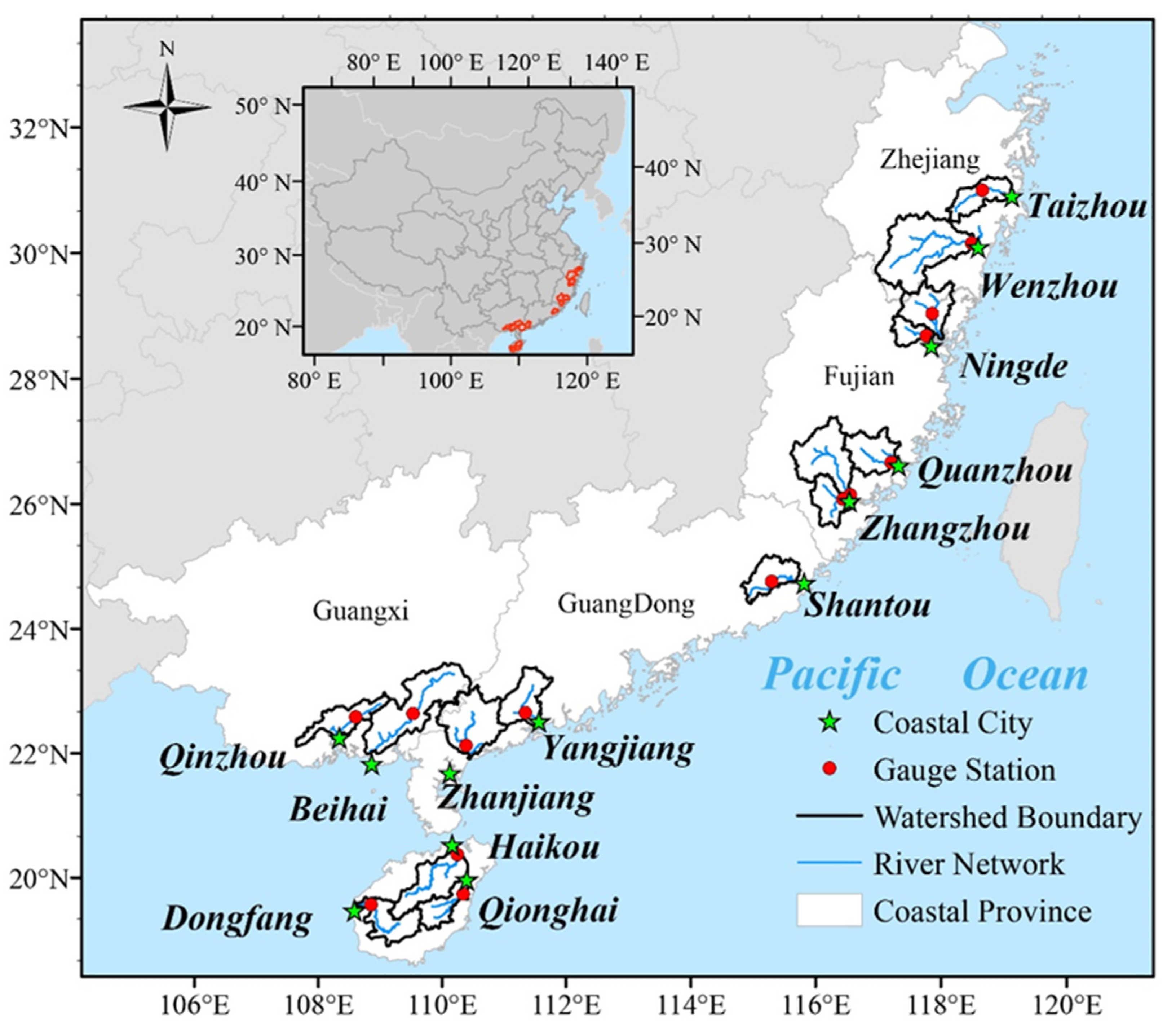
This study selected fifteen coastal-estuarine regions in the coastal southeastern China, including the coastal area of the Chinese mainland and Hainan Island of southeastern China (Figure 1) (defined as the region within 106° E to 120° E and 18° N to 32° N; referenced to the World Geodetic System 1984, WGS84). The selected coastal-estuarine regions satisfy the condition that the ratio of the tropical-cyclone-induced rainfall to the total rainfall in the catchment that drains freshwater into ocean is greater than 10%, according to the analysis of spatiotemporal variation in typhoon rainfall over South China [46]. Figure 1 shows the locations of catchments that drains freshwater into ocean and coastal cities in the selected coastal-estuarine regions. The fifteen coastal-estuarine regions are located in subtropical monsoon climate zone. Floods in these coastal-estuarine regions mainly occur from May to September. In the flood season, heavy rainstorms are the major cause of floods in this region, and they are dominated by two distinct systems: East Asian monsoon and tropical cyclone in North Pacific Ocean.
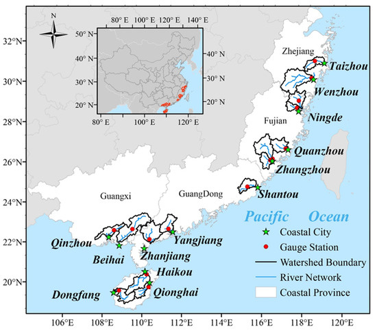
Figure 1.
Locations of the catchments that drain freshwater into ocean and coastal cities in the selected coastal-estuarine regions.
Every coastal-estuarine region has only one corresponding gauge station, and then it was named after the corresponding gauge station in this study. Fifteen hydrological stations are located in fifteen watershed outlets (Figure 1). The daily river discharge data from 1960 to 2015 were obtained from the Hydrology and Water Resources Bureau, but the data in several years are missing (Table 1). The daily sea surface height in the China’s seas and the adjacent areas (defined as the region within 99° E to 150° E and 10° S to 52° N; referenced to the World Geodetic System 1984, WGS84) from 1960 to 2015 was from a regional re-analysis product (CORA) published by National Marine Data Center [47]. The horizontal resolution changes with locations. The finest horizontal resolution is (1/8)° latitude ×(1/8)° longitude and the coarsest horizontal resolution is (1/2)° latitude ×(1/2)° longitude.

Table 1.
Basic characteristics of the selected coastal-estuarine regions.
Daily precipitation data was from the 0.25° × 0.25° China Gauge-based Daily Precipitation (CGDPA) product [48]. Digital elevation data with a resolution of 90 m were downloaded from the shuttle radar topography mission (SRTM) database [49]. The catchment boundaries were extracted from the DEM, and the daily basin-average rainfall was calculated based on the catchment boundaries and CGDPA. Characteristics of tropical cyclones, including the central location, maximum sustained wind and minimum sea level pressure, were collected from the Shanghai Typhoon Institute (STI) of the China Meteorological Administration, China. The available period of tropical cyclone data was from 1960 to 2015, and the temporal resolution was 6 h [50].
2.2. Methodology
2.2.1. Extraction of Compound Flood Events
Prior to the construction of bivariate probability distribution, the compound flood events should be extracted. For a coastal-estuarine region, a compound flood event is defined by the pair of two variables: river discharge and sea level. The river discharge time series is the collected data of the corresponding gauge station in a coastal-estuarine region which is given in Table 1. In terms of sea level time series, the distance between every grid in CORA and the gauge station was calculated and the sea surface height in the closest grid in CORA was regarded as the sea level time series for the coastal-estuarine region.
Based on daily river discharge and daily sea level time series, we used the Ppeak-over-threshold (POT) approach (i.e., all values selected above a given threshold) [51] to extract compound flood events following the study by Ward et al. [52]. Firstly, the high river discharge occurring two times per year on average were selected from daily river discharge time series. Then, the corresponding sea level is defined as maximum daily sea level within 1 day of the high river discharge.
2.2.2. Construction of Bivariate Probability Distribution
Based on selected compound flood events, bivariate probability distribution of river discharge and sea level was constructed by copulas. More information about copulas and their properties can be found in Nelsen [53] and Joe [54]. There exists a copula C such that:
where represents the bivariate probability distribution; denotes marginal univariate distribution of x, denotes marginal univariate distribution of y; X represents river discharge(m3/s) and Y represents sea level (m).
We used a MATLAB toolbox, Multivariate Copula Analysis Toolbox (MvCAT) developed by Sadegh et al. [55] to model bivariate probability distribution. MvCAT includes a wide range of copula families with different levels of complexity and employs a Bayesian framework with a residual-based Gaussian likelihood function for inferring copula parameters. The main advantages of MvCAT are introducing a hybrid-evolution Markov Chain Monte Carlo (MCMC) approach designed for numerical estimation of the posterior distribution of copula parameters, and enabling the community to explore a wide range of copulas and evaluate them relative to the fitting uncertainties. However, MvCAT is a lack of goodness-of-fit test for bivariate probability distribution functions testing the hypothesis that the specified distribution statistically fits with the data. We combined MvCAT with goodness-of-fit tests in this study.
According to guidelines for multivariate analysis and design in coastal and off-shore engineering [56], the steps that should be carried out for modeling bivariate probability distribution are as follows:
- Univariate analysis: McVAT was used to select the “best” marginal univariate distributions and , respectively. McVAT employs 17 different continuous marginal distribution functions (Beta, Birnbaum-Saunders, Exponential, Extreme value, Gamma, Generalized extreme value, Generalized Pareto, Inverse Gaussian, Logistic, Log-logistic, Lognormal, Nakagami, Normal, Rayleigh, Rician, T location-scale and Weibull) as candidate marginal distributions. The distribution functions are given in Table S1. The parameters of all candidate marginal distributions were estimated through a maximum likelihood algorithm based on observed time series of one variable. Kolmogorov–Smirnov goodness-of-fit test [57] was then employed to statistically examine the hypothesis that data was sampled from the fitted distribution at 5% significance level. The “best” marginal univariate distribution was picked out from non-rejected candidate marginal distributions based on the Akaike information criterion (AIC) [58]. Nash–Sutcliffe efficiency (NSE) between theoretical and empirical probabilities [56] was applied to evaluate the performance of fitted marginal univariate distribution.
- Dependency analysis: The estimates of the Kendall Rank correlation coefficient [59] was computed between river discharge X and sea level Y, and, also, the corresponding independence tests was assessed at 10% significance level. If the p-value is larger than 10%, river discharge X and sea level Y are independent. Otherwise, they are significantly correlated.
- Bivariate Analysis: If river discharge X and sea level Y were correlated, McVAT providing 26 copula functions were used as candidate bivariate distributions. The candidate bivariate distributions include Gaussian, T, Clayton, Frank, Gumbel, Independence Ali–Mikhail–Haq, Joe, Farlie–Gumbel–Morgenstern, Gumbel–Barnett, Plackett, Cuadras–Auge, Raftery, Shih–Louis, Linear-Spearman, Cubic, Burr, Nelsen, Galambos, Marshall–Olkin, Fischer–Hinzmann, Roch–Alegre, Fischer–Kock, BB1, BB5 and Tawn copula functions. The equation of these functions can be found in [56]. The parameters of all candidate bivariate distributions were estimated by a Bayesian framework with a residual-based Gaussian likelihood function. Cramér–von Mises (CM) test was used to goodness of fit test of copula functions. Consistent with univariate analysis, the “best” copula function was chosen from non-rejected candidate couple functions on the Akaike information criterion (AIC) and NSE was applied to evaluate the performance of fitted copulas.
- Construction of bivariate probability distribution: if river discharge X and sea level Y are independent, then the bivariate probability distribution can be described by independent joint distribution as:where and are “best” marginal univariate distributions.If river discharge X and sea level Y were correlated, the bivariate probability distribution can be described as Equation (1). The copula C in Equation (1) is replaced with the “best” copula function and in Equation (1) are replaced with and , respectively.
2.2.3. Modeling a Flood Typing-Based Bivariate Distribution
The modeling processes involves four steps: (1) Extraction of compound flood events: see Section 2.2.1. (2) Attribution of flood types: in this study, compound flood events were classified into three types: “non-TC-induced flood events”, “non-TC and TC-induced flood events (mixed)” and “TC-induced flood events”. Based on river discharge time series in compound flood events, we used the identification approach of flood types proposed by Lu et al. [45] to classify compound flood events into three types. This approach identified flood types by linking flooding to rainfall and was successfully applied in the southeastern coastal region of China. The main advantage of this approach lies in the detection of flood caused by remote TC rainfall which cannot be detected by more traditional method such as Villarini’s method [41]. The data needed in this approach is daily basin-average rainfall, river discharge time series, and tropical cyclone data. The details of this method can be found in Lu et al. [45]. (3) Construction of bivariate probability distribution: the construction of bivariate probability distribution in Section 2.2.2 was performed: (i) for non-TC-induced flood events; (ii) for mixed flood events; (iii) for TC-induced flood events. (4) Modeling a flood typing-based bivariate distribution: the flood typing-based bivariate distribution is described through a weighting of the bivariate probability distribution obtained in (2):
where , and represent bivariate probability distribution for non-TC-induced flood events, mixed flood events and TC-induced flood events, respectively. The parameter equals the ratio of the number of non-TC-induced flood events to the number of all compound flood events. The parameter equals the ratio of the number of mixed flood events to the number of all compound flood events.
To evaluate the impacts of mixed flood-generating mechanisms on bivariate probability distribution, the performance of the flood typing-based bivariate distribution (Section 2.2.3) was compared with that of bivariate probability distribution (Section 2.2.2) in all coastal-estuarine regions. The flood typing-based bivariate distribution is a bivariate probability distribution model that takes different flood-generating mechanisms into account, whereas, the bivariate probability distribution does not consider flood-generating mechanism. The performance was quantified through NSE between theoretical joint probability and empirical joint probability. The Mann–Whitney U test [60] was employed to examine the statistical significance of the differences of NSE values calculated by flood typing-based bivariate distribution and bivariate probability distribution. The p-value in the Mann–Whitney U test is larger than 0.5 means that the NSE values calculated by two approaches are not significantly different at 0.5 significance level. It indicates that the impacts of flood-generating mechanisms on coastal flood risk is limited.
2.2.4. Bivariate Return Period and Bivariate Design Value
The bivariate return period and bivariate design value were used to assess the coastal flooding risk. After modeling the bivariate probability distribution, the bivariate return period can be derived from univariate return period. The univariate return period is computed as:
where is the cumulative probability distribution of X; n is the length (in years) of the considered time series; t is the number of events.
Then, the bivariate return period is computed as Sadegh et al. [61]:
where is the bivariate probability distribution of X and Y; n is the length (in years) of the considered time series; t is the number of compound flood events.
Given a bivariate return period is chosen, many pairs of values (x, y) can have the same bivariate return period. The bivariate design values for x and y can be obtained by most-likely design realization method [62]. This approach introduces a weighting function which specifies the point over the critical layer with the greatest value of the joint probability density function . The design value corresponding to bivariate return period can be described as:
To evaluate the compounding effect of river discharge and water level on coastal flood risk, we employed two approaches: copulas and independent joint distribution to establish the bivariate probability distribution in coastal-estuarine regions where river discharge and water level were significantly correlated. In the former, coastal flood resulted from the compounding effects of two variables. However, in the latter, coastal flood was caused solely by a single variable and the compounding effects of two variables on flood risk was neglected. Then, the bivariate return period and bivariate design values calculated by two approaches were compared.
3. Results
3.1. Bivariate Probability Distribution of Compound Flood Events
The results of best marginal function and goodness-of-fit test in the univariate analysis were given in Table S2. All chosen marginal function passed Kolmogorov–Smirnov goodness-of-fit test (p-value > 0.05 at 5% significance level) and the NSE values in all coastal-estuarine regions were larger than 0.97. It means the chosen best marginal function provides a very good fit to the data. The best function of river discharge in all coastal-estuarine regions, except Jiaji, was generalized extreme value function, whereas that of sea level varied, which means that the fitted distributions of river discharge were different from that of sea level. It can also be found in a more visual way (See Figures S1 and S2).
Table 2 showed the Kendall tao rank correlation coefficients and p-value of independent tests between river discharge and sea level in the coastal-estuarine regions. It indicates that in 5 of 15 coastal-estuarine regions, river discharge and sea level were significantly correlated but in a weak correlation (Kendall tao rank correlation coefficient of 0.11~0.23). In the rest 10 coastal-estuarine regions, the two variables were independent.
Table 2.
Correlation coefficients and independent tests between river discharge and sea level.
We used independent joint distribution to fit the bivariate probability distribution and applied CM test to test the joint distribution in all coastal-estuarine regions. The results were shown in Figure 2. The critical 5% level is indicated by a dashed line, the p-values of CM test is smaller than the critical level means that the independent joint distribution cannot describe the dependence structure of river discharge and sea level. It can be seen that in 10 coastal-estuarine regions, where river discharge and sea level were independent, the independent joint distribution passed the CM test. However, in the remaining 5 coastal-estuarine regions, where the two variables were correlated, the independent joint distribution cannot fit with the data. This demonstrates the necessary of using copula functions to describe the dependence structure of river discharge and sea level in those 5 coastal-estuarine regions.
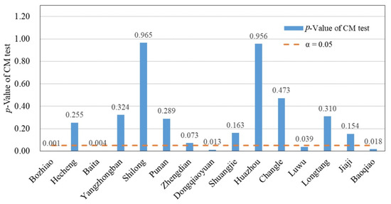
Figure 2.
Goodness-of-fit of independent joint distribution in all coastal-estuarine regions.
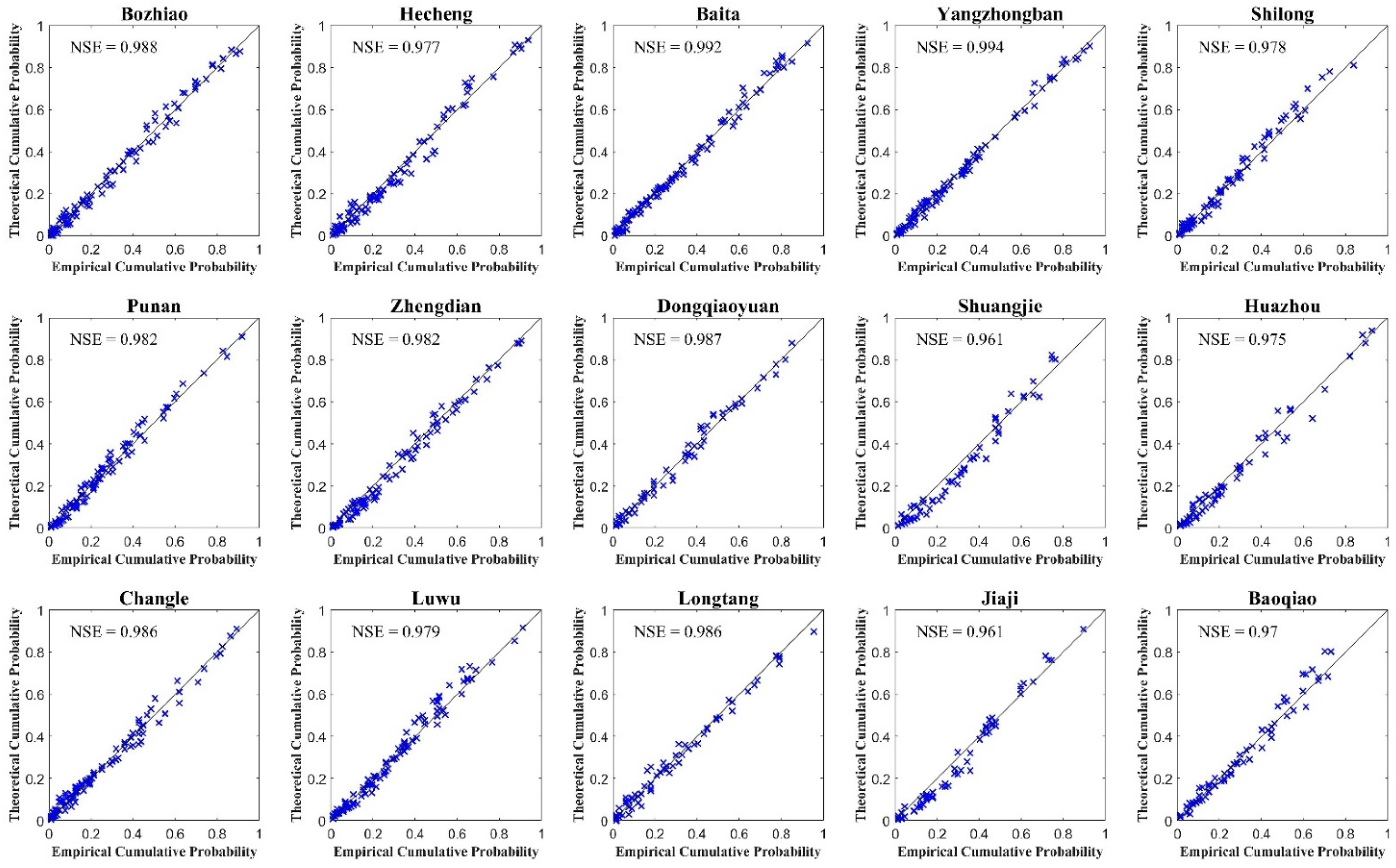
The goodness-of-fit tests of the copula function in 5 coastal-estuarine regions were given in Table S3. It can be seen that most of candidate copula functions passed CM test in 5 coastal-estuarine regions. The best copula function in Bozhiao was the Ali–Mikhail–Haq function while that in Baita was the Farlie–Gumbel–Morgenstern function. The best copula function in other three regions was Clayton function (see Table S4). The P–P plots between constructed bivariate probability distribution and empirical joint probability were shown in Figure 3. The NSE values of bivariate joint probability and empirical joint probability is above 0.96, which indicates that constructed bivariate probability distributions have given a better fit for compound flood events.
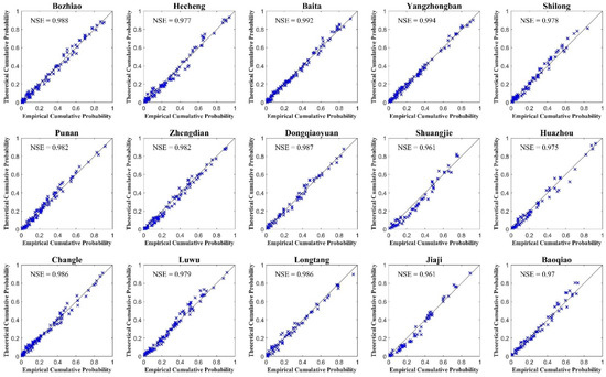
Figure 3.
P–P plot of the bivariate probability distribution.
3.2. Compound Flood Events per Flood Type
Figure 4 showed the percentages of TC-induced, non-TC-induced and mixed-induced flood events to total compound flood events in coastal-estuarine regions. The percentages of TC-induced flood events ranged from 18% to 55%, while that of non-TC-induced flood events ranged from 49% to 72%. The percentages of mixed-induced flood events were below 25%. Non-TC-induced flood occupied larger proportions in the coastal area of China mainland (all coastal-estuarine regions except Longtang, Jiaji and Baoqiao), while non-TC floods dominated in Hainan Island (including Longtang, Jiaji and Baoqiao). Figure 5 displayed the percentage of mixed, non-TC-induced and TC-induced flood events per month in coastal-estuarine regions. The highest percentages of TC-induced floods appeared in August, while that of non-TC-induced floods appeared in June. However, mixed floods mostly occurred in both June and August. It can be seen that the seasonality of three flood types were different, which confirms the necessity to analyze the impact of mixed flood-generating mechanisms on bivariate probability distribution.
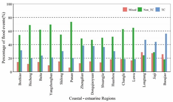
Figure 4.
Percentage of mixed, non-TC-induced and TC-induced flood events in coastal-estuarine regions.
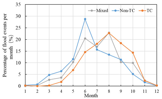
Figure 5.
Percentage of mixed, non-TC-induced and TC-induced flood events per month in coastal-estuarine regions.
3.3. Impacts of Mixed Flood-Generating Mechanisms on Bivariate Probability Distribution
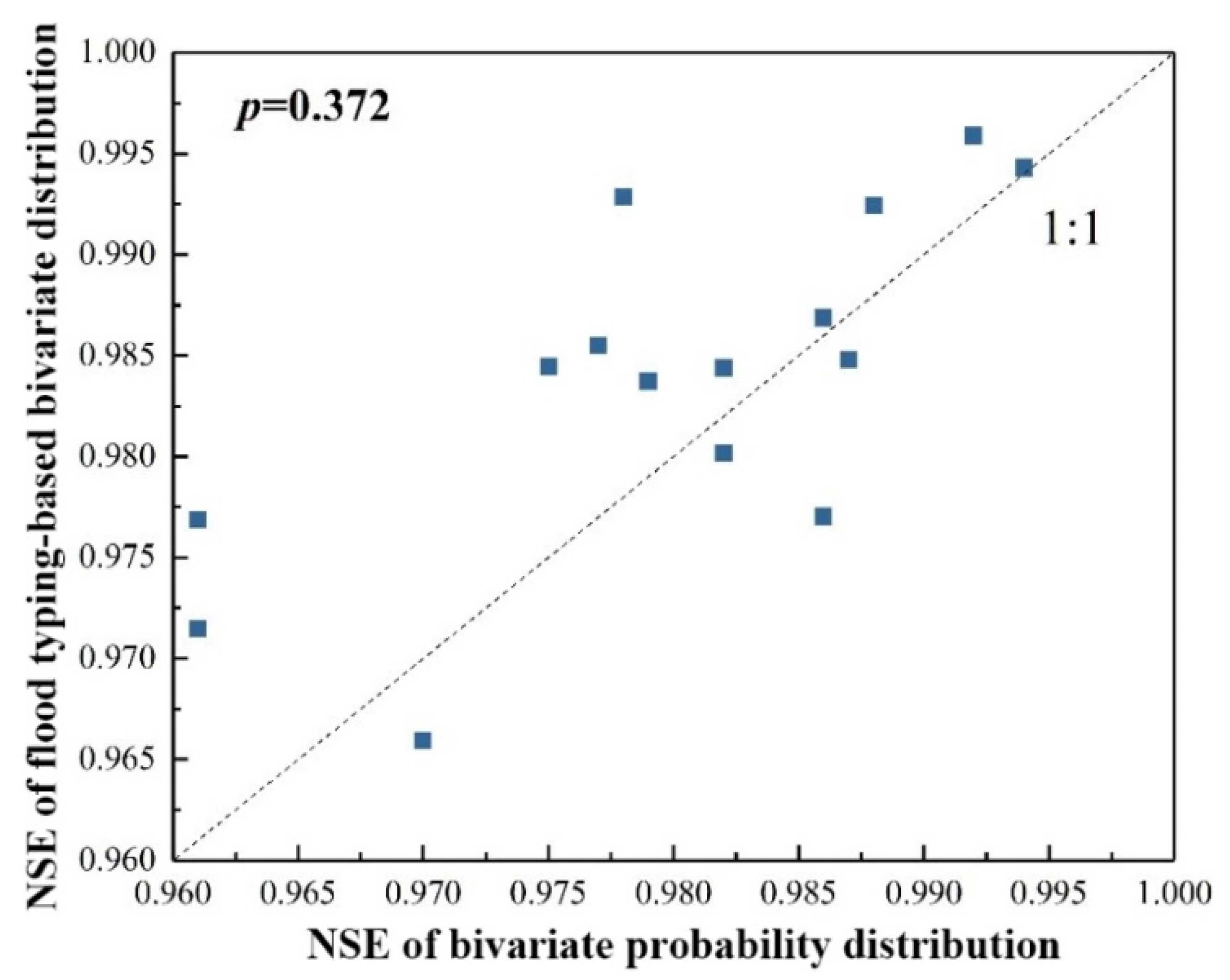
A flood typing-based bivariate distribution was built in 15 coastal-estuarine regions. The performance of the flood typing-based bivariate distribution and bivariate probability distribution was given in Figure 6. In 11 out of 15 coastal-estuarine regions, the NSE values of the flood typing-based bivariate distribution was larger than that of the bivariate probability distribution. The p-value in the Mann–Whitney U test is larger than 0.5. It means that the performance of flood typing-based bivariate distribution was not significantly better than the bivariate probability distribution in coastal-estuarine regions. In 11 out of 15 coastal-estuarine regions, the flood typing-based bivariate distribution still performs better than the bivariate probability distribution in terms of NSE values. However, in the other 4 coastal-estuarine regions, it comes to the contradictory conclusion.

Figure 6.
The performance of flood typing-based bivariate distribution and bivariate probability distribution.
3.4. Compounding Effects on Bivariate Return Period and Bivariate Design Value
The bivariate probability distributions were built based on the best fitted copula function in 5 coastal-estuarine regions (Bozhiao, Baita, Dongqiaoyuan, Luwu and Baoqiao) where the river discharge and sea level were correlated. Then, the bivariate return periods and bivariate design values were calculated based on constructed bivariate probability distributions. For the sake of comparison, the bivariate return periods and bivariate design values were also calculated based on independent joint distribution in 5 coastal-estuarine regions. Assuming that the univariate return period for the two variables was the same, the bivariate return periods were calculated by Equation (4) when the univariate return period equals to 5, 10, 20, 50 and 100 years, respectively. The results were shown in Figure 7. The dash line represents the return periods calculated by independent joint distribution and the bar represents the return periods calculated by the best fitted copula function. It can be seen that the bivariate return periods calculated by copula and independent joint distribution had little difference. This indicates that compounding impacts of river discharge and sea level may inappropriately characterize the coastal flood risk, but had limited impact on bivariate return periods.
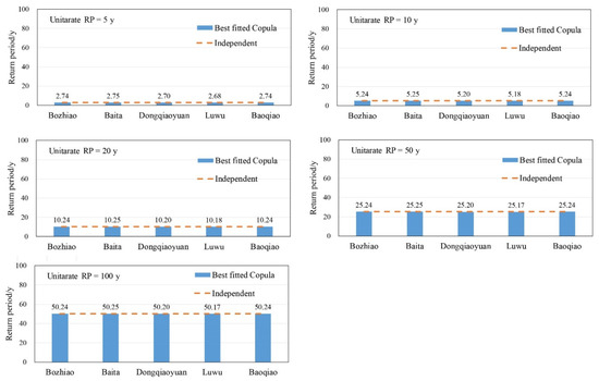
Figure 7.
Bivariate return periods calculated by the copula function and independent joint distribution.
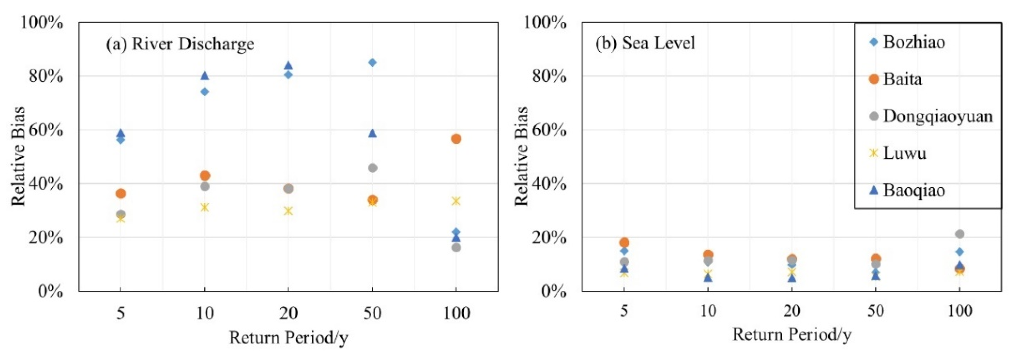
The bivariate design values calculated by best fitted copula function and independent joint distribution were in Table 3. It can be seen that, for a certain return period, either design river discharge or design sea level calculated by copula function was larger than that calculated by independent joint distribution. For the sake of illustration, the relative bias between bivariate design values calculated by copula function and independent joint distribution was shown in Figure 8. The relative bias of design values for both variables larger than zero indicates that the design values in consideration of compounding effects of two variables were larger than that when neglecting the compounding effects. It means that compounding effects of river discharge and sea level heavily influenced coastal flood risk in terms of design values. Ignoring compounding effects of river discharge and sea level leads to significant underestimation of design values. The relative bias of design river discharge was larger than 15% when the bivariate return period ranges from 5 to 100 years. The largest bias of design river discharge reached to 84%. The relative bias of design sea level was less than 20%. The smallest bias of design sea level was nearly 5%. The relative bias of design river discharge generally was larger than that of design sea level. It can be inferred that comparing with design sea level, the compounding effects of river discharge and sea level had stronger influence on design river discharge.
Table 3.
Bivariate design values calculated by best fitted copula function and independent joint distribution.
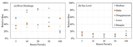
Figure 8.
Relative bias of design values of (a) River discharge and (b) Sea level calculated by copula function and independent joint distribution.
4. Discussion
The dependence between river discharge and sea level was significant, but had limited impact on bivariate return periods in the coastal-estuarine region of southeastern China. It is consistent with the findings by Ward et al. [52] that significant dependence between observed high sea-levels and high river discharge exists for deltas and estuaries around the globe. The study region in Ward et al. [52] does not cover the estuaries of China. Therefore, this study can extend the understanding of dependence between sea level and river discharge over the globe. Compared with this study, a different conclusion that the river discharge and sea level was highly correlated was obtained in other coastal regions such as Britain [17] and USA [5]. This may be due to the different dataset of sea level data that used, with daily re-analysis data being used in this study, and hourly observed data being used in Svensson and Jones [17] and Moftakhari et al. [5]. The daily re-analysis data resulted from the combination of astronomical tide and storm surge processes while hourly observed data represents the variability of storm surge process. As only storm surge process is physically associated with high river discharge [18], using daily re-analysis sea level data may lead to lower dependence compared to when using hourly observed sea level data. An hourly sea level dataset should be further used to re-evaluate the dependency between river discharge and sea level in the coastal-estuarine region of southeastern China.
Despite of weak dependence between river discharge and sea level, the dependence between river discharge and sea level strongly influenced bivariate design values. Ignoring the compounding effect of river discharge and sea level leads to underestimation of design values. This finding is consistent with studies by Bevacqua et al. [34] and Marsaglia et al. [57]. Both studies used the dependence structure of river discharge and sea level as the boundary conditions of hydrodynamical model of coastal flooding. Besides, the dependence between river discharge and sea level was also considered when assessing the risk of coastal flooding [4,7,63]. However, whether river discharge and sea level can be treated independently or not is still debated. Klerk et al. [7] stated that a significant dependence is more likely in small coastal catchments which have quick rainfall-runoff process response time. The reason for the dispute may be difficulties in quantifying the impact due to limited data length. The limited data availability is a limitation in this study. The available record length of the observed data in this study ranges from 34 to 54 years. Dung et al. [64] quantified the uncertainties inherent with bivariate probability distribution and stated that a series length of about 200 years was needed to reduce the uncertainty to an acceptable range in bivariate design values estimation. For practical purposes, the high sampling uncertainty in bivariate design values should be considered by decision makers and water managers.
This study found that the performance of flood typing-based bivariate distribution was not significantly better than the bivariate probability distribution in coastal-estuarine regions. In 11 out of 15 coastal-estuarine regions, the flood typing-based bivariate distribution still performs better than the bivariate probability distribution in terms of NSE values. This may be due to that additional information such as tropical cyclone data was used in the flood typing-based approach, which can allow for more reliable flood probability estimation [65,66]. This finding is consistent with previous flood risk analysis in consideration of different flood types [43,67]. However, in other 4 coastal-estuarine regions, it comes to the contradictory conclusion. The possible reason is that the flood typing-based bivariate distribution involves more parameters and has lower sample size, which leads to an increased parameter and sampling uncertainty of the flood probability estimation [68,69]. The applicability of the flood typing-based bivariate distribution varied in different regions and hence the benefit of the higher NSE and the disadvantage of the larger uncertainty have to be balanced. An innovative flood typing-based method balancing better model performance and lower uncertainty should be developed.
5. Conclusions
This study aims to analyze the impact of mixed flood-generating mechanisms on bivariate probability distribution and evaluate the compounding effect of river discharge and sea level on coastal flood risk. The major findings of this study are summarized as follows.
- (1)
- With regard to compound flood events per flood type, the percentages of TC-induced flood events ranged from 18% to 55%, while that of non-TC-induced flood events ranged from 49% to 72%. The percentages of mixed-induced flood events were below 25%. Non-TC-induced flood occupied larger proportions in in the coastal area of China mainland (all coastal-estuarine regions except Longtang, Jiaji and Baoqiao), while non-TC floods dominated in Hainan Island (including Longtang, Jiaji and Baoqiao). The highest percentages of TC-induced floods appeared in August, while that of non-TC-induced floods appeared in June. However, mixed floods mostly occurred in both June and August. The seasonality of three flood types were different, which confirms the necessity to analyze the impact of mixed flood-generating mechanisms on bivariate probability distribution.
- (2)
- MvCAT combined with goodness-of fit tests were used to construct bivariate probability distributions in 15 coastal-estuarine regions of Southeastern China and a flood typing-based bivariate distribution was built in 15 coastal-estuarine regions. In 11 out of 15 coastal-estuarine regions, the flood typing-based bivariate distribution still performs better than the bivariate probability distribution in terms of NSE values. However, in the other 4 coastal-estuarine regions, it comes to the contradictory conclusion. The performance of flood typing-based bivariate distribution was not significantly better than the bivariate probability distribution in coastal-estuarine regions based on the Mann–Whitney U test. The applicability of the flood typing-based bivariate distribution varied in different regions, and hence, the benefit of the higher NSE and the disadvantage of the larger uncertainty have to be balanced.
- (3)
- The compounding impacts of river discharge and sea level had limited impact on bivariate return periods, whereas had greater impact on coastal flooding risk in terms of design values. In terms of design values, either the design river discharge or design sea level in consideration of compounding effects of river discharge and sea level was larger than that when neglecting compounding effects. Ignoring compounding effects of river discharge and sea level leads to significant underestimation of design values. Comparing with design sea level, the compounding effects of river discharge and sea level had stronger influence on design river discharge.
Supplementary Materials
The following supporting information can be downloaded at: https://www.mdpi.com/article/10.3390/atmos13020238/s1, Figure S1. Empirical distribution functions (blue markers) and theoretical distribution function (red lines) of river discharge, Figure S2. Empirical distribution functions (blue markers) and theoretical distribution function (red lines) of sea, Table S1. Goodness-of-fit tests of marginal distribution in the univariate analysis, Table S2. Goodness-of-fit tests of marginal distribution in the univariate analysis, Table S3. Goodness-of-fit tests of Copula function in the bivariate analysis, Table S4. The best fitted Copula function in 5 coastal-estuarine regions.
Author Contributions
Conceptualization, W.L.; writing—original draft preparation, W.L. and H.W.; writing—review and editing, W.L. and L.T.; supervision, D.Y. and Z.L.; funding acquisition, D.Y. and Z.L. All authors have read and agreed to the published version of the manuscript.
Funding
This research was funded by the National Natural Science Foundation of China (No. 41661144031), Open Research Fund Program of State key Laboratory of Hydroscience and Engineering (sklhse-2021-A-05), the scientific project of China Three Gorges Corporation (Grant No. 202003098).
Institutional Review Board Statement
Not applicable.
Informed Consent Statement
Not applicable.
Data Availability Statement
The datasets analyzed during the current study are available from the corresponding author on reasonable request.
Acknowledgments
The authors are grateful to the anonymous reviewers for their invaluable comments and for editing a previous draft of the manuscript.
Conflicts of Interest
The authors declare no conflict of interest.
References
- Emanuel, K. Increasing destructiveness of tropical cyclones over the past 30 years. Nature 2005, 436, 686–688. [Google Scholar] [CrossRef] [PubMed]
- Webster, P.J.; Holland, G.J.; Curry, J.A.; Chang, H.R. Changes in tropical cyclone number, duration, and intensity in a warming environment. Science 2005, 309, 1844–1846. [Google Scholar] [CrossRef] [PubMed] [Green Version]
- Woodruff, J.D.; Irish, J.L.; Camargo, S.J. Coastal flooding by tropical cyclones and sea-level rise. Nature 2013, 504, 44–52. [Google Scholar] [CrossRef] [PubMed] [Green Version]
- Kew, S.F.; Selten, F.M.; Lenderink, G.; Hazeleger, W. The simultaneous occurrence of surge and discharge extremes for the Rhine delta. Nat. Hazards Earth Syst. Sci. 2013, 13, 2017–2029. [Google Scholar] [CrossRef] [Green Version]
- Moftakhari, H.R.; Salvadori, G.; AghaKouchak, A.; Sanders, B.F.; Matthew, R.A. Compounding effects of sea level rise and fluvial flooding. Proc. Natl. Acad. Sci. USA 2017, 114, 9785–9790. [Google Scholar] [CrossRef] [Green Version]
- Zscheischler, J.; Westra, S.; van den Hurk, B.J.J.M.; Seneviratne, S.I.; Ward, P.J.; Pitman, A.; AghaKouchak, A.; Bresch, D.N.; Leonard, M.; Wahl, T.; et al. Future climate risk from compound events. Nat. Clim. Chang. 2018, 8, 469–477. [Google Scholar] [CrossRef]
- Klerk, W.J.; Winsemius, H.C.; van Verseveld, W.J.; Bakker, A.M.R.; Diermanse, F.L.M. The co-incidence of storm surges and extreme discharges within the Rhine–Meuse Delta. Environ. Res. Lett. 2015, 10, 035005. [Google Scholar] [CrossRef] [Green Version]
- Wahl, T.; Jain, S.; Bender, J.; Meyers, S.D.; Luther, M.E. Increasing risk of compound flooding from storm surge and rainfall for major US cities. Nat. Clim. Chang. 2015, 5, 1093–1097. [Google Scholar] [CrossRef]
- Zhang, W.; Chang, W.J.; Zhu, Z.C.; Hui, Z. Landscape ecological risk assessment of Chinese coastal cities based on land use change. Appl. Geogr. 2020, 117, 102174. [Google Scholar] [CrossRef]
- Jongman, B.; Ward, P.J.; Aerts, J.C.J.H. Global exposure to river and coastal flooding: Long term trends and changes. Glob. Environ. Chang. 2012, 22, 823–835. [Google Scholar] [CrossRef]
- Hinkel, J.; Lincke, D.; Vafeidis, A.T.; Perrette, M.; Nicholls, R.J.; Tol, R.S.J.; Marzeion, B.; Fettweis, X.; Ionescu, C.; Levermann, A. Coastal flood damage and adaptation costs under 21st century sea-level rise. Proc. Natl. Acad. Sci. USA 2014, 111, 3292–3297. [Google Scholar] [CrossRef] [PubMed] [Green Version]
- Neumann, B.; Vafeidis, A.T.; Zimmermann, J.; Nicholls, R.J. Future Coastal Population Growth and Exposure to Sea-Level Rise and Coastal Flooding—A Global Assessment. PLoS ONE 2015, 10, e0118571. [Google Scholar] [CrossRef] [PubMed] [Green Version]
- Zheng, F.; Leonard, M.; Westra, S. Application of the design variable method to estimate coastal flood risk. J. Flood Risk Manag. 2017, 10, 522–534. [Google Scholar] [CrossRef]
- Kasiviswanathan, K.S.; He, J.; Tay, J.-H. Flood frequency analysis using multi-objective optimization based interval estimation approach. J. Hydrol. 2017, 545, 251–262. [Google Scholar] [CrossRef]
- Salvadori, G.; De Michele, C. Frequency analysis via copulas: Theoretical aspects and applications to hydrological events. Water Resour. Res. 2004, 40. [Google Scholar] [CrossRef]
- De Michele, C.; Salvadori, G.; Canossi, M.; Petaccia, A.; Rosso, R. Bivariate statistical approach to check adequacy of dam spillway. J. Hydrol. Eng. 2005, 10, 50–57. [Google Scholar] [CrossRef]
- Svensson, C.; Jones, D.A. Dependence between sea surge, river flow and precipitation in south and west Britain. Hydrol. Earth Syst. Sci. 2004, 8, 973–992. [Google Scholar] [CrossRef] [Green Version]
- Zheng, F.; Westra, S.; Sisson, S.A. Quantifying the dependence between extreme rainfall and storm surge in the coastal zone. J. Hydrol. 2013, 505, 172–187. [Google Scholar] [CrossRef]
- Xu, H.; Xu, K.; Lian, J.; Ma, C. Compound effects of rainfall and storm tides on coastal flooding risk. In Stochastic Environmental Research and Risk Assessment; Springer: Berlin/Heidelberg, Germany, 2019. [Google Scholar]
- Ganguli, P.; Paprotny, D.; Hasan, M.; Güntner, A.; Merz, B. Projected Changes in Compound Flood Hazard from Riverine and Coastal Floods in Northwestern Europe. Earth’s Future 2020, 8, e2020EF001752. [Google Scholar] [CrossRef]
- Couasnon, A.; Eilander, D.; Muis, S.; Veldkamp, T.I.E.; Haigh, I.D.; Wahl, T.; Winsemius, H.C.; Ward, P.J. Measuring compound flood potential from river discharge and storm surge extremes at the global scale. Nat. Hazards Earth Syst. Sci. 2020, 20, 489–504. [Google Scholar] [CrossRef] [Green Version]
- Eilander, D.; Couasnon, A.; Ikeuchi, H.; Muis, S.; Yamazaki, D.; Winsemius, H.C.; Ward, P.J. The effect of surge on riverine flood hazard and impact in deltas globally. Environ. Res. Lett. 2020, 15, 104007. [Google Scholar] [CrossRef]
- Santos, V.M.; Casas-Prat, M.; Poschlod, B.; Ragno, E.; van den Hurk, B.; Hao, Z.; Kalmár, T.; Zhu, L.; Najafi, H. Statistical modelling and climate variability of compound surge and precipitation events in a managed water system: A case study in the Netherlands. Hydrol. Earth Syst. Sci. 2021, 25, 3595–3615. [Google Scholar] [CrossRef]
- Sanuy, M.; Rigo, T.; Jiménez, J.A.; Llasat, M.C. Classifying compound coastal storm and heavy rainfall events in the north-western Spanish Mediterranean. Hydrol. Earth Syst. Sci. 2021, 25, 3759–3781. [Google Scholar] [CrossRef]
- Wu, W.; McInnes, K.; O’Grady, J.; Hoeke, R.; Leonard, M.; Westra, S. Mapping Dependence between Extreme Rainfall and Storm Surge. J. Geophys. Res. Ocean. 2018, 123, 2461–2474. [Google Scholar] [CrossRef]
- Lian, J.J.; Xu, K.; Ma, C. Joint impact of rainfall and tidal level on flood risk in a coastal city with a complex river network: A case study for Fuzhou city, China. Hydrol. Earth Syst. Sci. Discuss. 2012, 9, 7475–7505. [Google Scholar] [CrossRef] [Green Version]
- Xu, K.; Ma, C.; Lian, J.; Bin, L. Joint Probability Analysis of Extreme Precipitation and Storm Tide in a Coastal City under Changing Environment. PLoS ONE 2014, 9, e109341. [Google Scholar] [CrossRef]
- Wahl, T.; Mudersbach, C.; Jensen, J. Assessing the hydrodynamic boundary conditions for risk analyses in coastal areas: A multivariate statistical approach based on Copula functions. Nat. Hazards Earth Syst. Sci. 2012, 12, 495–510. [Google Scholar] [CrossRef] [Green Version]
- Zheng, F.; Westra, S.; Leonard, M.; Sisson, S.A. Modeling dependence between extreme rainfall and storm surge to estimate coastal flooding risk. Water Resour. Res. 2014, 50, 2050–2071. [Google Scholar] [CrossRef]
- Apel, H.; Thieken, A.H.; Merz, B.; Blöschl, G. Flood risk assessment and associated uncertainty. Nat. Hazards Earth Syst. Sci. 2004, 4, 295–308. [Google Scholar] [CrossRef]
- Li, T.; Guo, S.; Lu, C.; Guo, J. Bivariate Flood Frequency Analysis with Historical Information Based on Copula. J. Hydrol. Eng. 2013, 18, 1018–1030. [Google Scholar] [CrossRef] [Green Version]
- Li, F.; Zheng, Q. Probabilistic modelling of flood events using the entropy copula. Adv. Water Resour. 2016, 97, 233–240. [Google Scholar] [CrossRef]
- Guo, A.; Chang, J.; Wang, Y.; Huang, Q.; Guo, Z.; Zhou, S. Bivariate frequency analysis of flood and extreme precipitation under changing environment: Case study in catchments of the Loess Plateau, China. Stoch. Environ. Res. Risk Assess. 2017, 32, 2057–2074. [Google Scholar] [CrossRef]
- Bevacqua, E.; Maraun, D.; Hobæk Haff, I.; Widmann, M.; Vrac, M. Multivariate statistical modelling of compound events via pair-copula constructions: Analysis of floods in Ravenna (Italy). Hydrol. Earth Syst. Sci. 2017, 21, 2701–2723. [Google Scholar] [CrossRef] [Green Version]
- Khanal, S.; Ridder, N.; de Vries, H.; Terink, W.; van den Hurk, B. Storm surge and extreme river discharge: A compound event analysis using ensemble impact modeling. Front. Earth Sci. 2019, 7, 224. [Google Scholar] [CrossRef]
- Moftakhari, H.; Schubert, J.E.; AghaKouchak, A.; Matthew, R.A.; Sanders, B.F. Linking statistical and hydrodynamic modeling for compound flood hazard assessment in tidal channels and estuaries. Adv. Water Resour. 2019, 128, 28–38. [Google Scholar] [CrossRef]
- Murphy, P.J. Evaluation of mixed-population flood-frequency analysis. J. Hydrol. Eng. 2001, 6, 62–70. [Google Scholar] [CrossRef]
- Todhunter, P.E. Uncertainty of the Assumptions Required for Estimating the Regulatory Flood: Red River of the North. ASCE 2011, 17, 1011–1020. [Google Scholar] [CrossRef]
- Singh, V.P.; Wang, S.X.; Zhang, L. Frequency analysis of nonidentically distributed hydrologic flood data. J. Hydrol. 2005, 307, 175–195. [Google Scholar] [CrossRef]
- Fischer, S.; Schumann, A.; Schulte, M. Characterisation of seasonal flood types according to timescales in mixed probability distributions. J. Hydrol. 2016, 539, 38–56. [Google Scholar] [CrossRef]
- Villarini, G.; Smith, J.A. Flood peak distributions for the eastern United States. Water Resour. Res. 2010, 46. [Google Scholar] [CrossRef] [Green Version]
- Yan, L.; Xiong, L.; Liu, D.; Hu, T.; Xu, C.-Y. Frequency analysis of nonstationary annual maximum flood series using the time-varying two-component mixture distributions. Hydrol. Process. 2017, 31, 69–89. [Google Scholar] [CrossRef]
- De Niel, J.; Demarée, G.; Willems, P. Weather Typing-Based Flood Frequency Analysis Verified for Exceptional Historical Events of Past 500 Years Along the Meuse River. Water Resour. Res. 2017, 53, 8459–8474. [Google Scholar] [CrossRef]
- Chang, C.-P.; Lei, Y.; Sui, C.-H.; Lin, X.; Ren, F. Tropical cyclone and extreme rainfall trends in East Asian summer monsoon since mid-20th century. Geophys. Res. Lett. 2012, 39, 8703–8719. [Google Scholar] [CrossRef]
- Lu, W.; Lei, H.; Yang, W.; Yang, J.; Yang, D. Comparison of floods driven by tropical cyclones and monsoons in the southeastern coastal region of China. J. Hydrometeorol. 2020, 21, 1589–1603. [Google Scholar] [CrossRef]
- Lee, M.-H. Influence of Tropical Cyclone Landfalls on Spatiotemporal Variations in Typhoon Season Rainfall over South China. Adv. Atmos. Sci. 2010, 2, 443–454. [Google Scholar] [CrossRef]
- Zhang, M.; Zhou, L.; Fu, H.; Jiang, L.; Zhang, X. Assessment of intraseasonal variabilities in China Ocean Reanalysis (CORA). Acta Oceanol. Sin. 2016, 35, 90–101. [Google Scholar] [CrossRef]
- Shen, Y.; Zhao, P.; Pan, Y.; Yu, J. A high spatiotemporal gauge-satellite merged precipitation analysis over China. J. Geophys. Res. Atmos. 2014, 119, 3063–3075. [Google Scholar] [CrossRef]
- Jarvis, A.; Reuter, H.I.; Nelson, A.; Guevara, E. Hole-filled seamless SRTM data V4. Tech. rep., International Centre for Tropical Agriculture (CIAT). 2008. Available online: https://cgiarcsi.community/data/srtm-90m-digital-elevation-database-v4-1/and (accessed on 2 January 2008).
- Ying, M.; Zhang, W.; Yu, H.; Lu, X.; Feng, J.; Fan, Y.; Zhu, Y.; Chen, D. An Overview of the China Meteorological Administration Tropical Cyclone Database. J. Atmos. Ocean. Technol. 2014, 31, 287–301. [Google Scholar] [CrossRef] [Green Version]
- Smith, R.L. Threshold Methods for Sample Extremes; Springer: Berlin/Heidelberg, Germany, 1984. [Google Scholar]
- Ward, P.J.; Couasnon, A.; Eilander, D.; Haigh, I.D.; Hendry, A.; Muis, S.; Veldkamp, T.I.E.; Winsemius, H.C.; Wahl, T. Dependence between high sea-level and high river discharge increases flood hazard in global deltas and estuaries. Environ. Res. Lett. 2018, 13, 84012. [Google Scholar] [CrossRef]
- Nelsen, R.B. An Introduction to Copulas; Springer: Berlin/Heidelberg, Germany, 2007. [Google Scholar]
- Joe, H. Dependence Modeling with Copulas; CRC Press: Boca Raton, FL, USA, 2014. [Google Scholar]
- Sadegh, M.; Ragno, E.; AghaKouchak, A. Multivariate Copula Analysis Toolbox (MvCAT): Describing dependence and underlying uncertainty using a Bayesian framework. Water Resour. Res. 2017, 53, 5166–5183. [Google Scholar] [CrossRef]
- Salvadori, G.; Tomasicchio, G.R.; D’Alessandro, F. Practical guidelines for multivariate analysis and design in coastal and off-shore engineering. Coast. Eng. 2014, 88, 1–14. [Google Scholar] [CrossRef]
- Marsaglia, G.; Tsang, W.W.; Wang, J. Evaluating Kolmogorov’s distribution. J. Stat. Softw. 2003, 8, 1–4. [Google Scholar] [CrossRef]
- Hjort, N.L. Model selection and model averaging. Cambridge Series in Statistical and Probabilistic Mathematics; Cambridge University Press: Cambridge, UK, 2008. [Google Scholar]
- Kendall, M.G. A new measure of rank correlation. Biometrika 1938, 30, 81–93. [Google Scholar] [CrossRef]
- Nachar, N. The Mann-Whitney U: A Test for Assessing Whether Two Independent Samples Come from the Same Distribution. Tutor. Quant. Methods Psychol. 2008, 4, 13–20. [Google Scholar] [CrossRef]
- Sadegh, M.; Moftakhari, H.; Gupta, H.V.; Ragno, E.; Mazdiyasni, O.; Sanders, B.; Matthew, R.; AghaKouchak, A. Multihazard Scenarios for Analysis of Compound Extreme Events. Geophys. Res. Lett. 2018, 45, 5470–5480. [Google Scholar] [CrossRef] [Green Version]
- Stamatatou, N.; Vasiliades, L.; Loukas, A. Bivariate Flood Frequency Analysis Using Copulas. Proceedings 2018, 2, 635. [Google Scholar] [CrossRef] [Green Version]
- van den Brink, H.W.; Können, G.P.; Opsteegh, J.D.; van Oldenborgh, G.J.; Burgers, G. Estimating return periods of extreme events from ECMWF seasonal forecast ensembles. Int. J. Climatol. 2005, 25, 1345–1354. [Google Scholar] [CrossRef]
- Dung, N.V.; Merz, B.; Bárdossy, A.; Apel, H. Handling uncertainty in bivariate quantile estimation–An application to flood hazard analysis in the Mekong Delta. J. Hydrol. 2015, 527, 704–717. [Google Scholar] [CrossRef]
- Merz, R.; Blöschl, G. Flood frequency hydrology: 1. Temporal, spatial, and causal expansion of information. Water Resour. Res. 2008, 44. [Google Scholar] [CrossRef] [Green Version]
- Merz, B.; Aerts, J.; Arnbjerg-Nielsen, K.; Baldi, M.; Becker, A.; Bichet, A.; Bloeschl, G.; Bouwer, L.M.; Brauer, A.; Cioffi, F.; et al. Floods and climate: Emerging perspectives for flood risk assessment and management. Nat. Hazards Earth Syst. Sci. 2014, 14, 1921–1942. [Google Scholar] [CrossRef] [Green Version]
- Fischer, S. A seasonal mixed-POT model to estimate high flood quantiles from different event types and seasons. J. Appl. Stat. 2018, 45, 2831–2847. [Google Scholar] [CrossRef]
- Serinaldi, F.; Kilsby, C.G. Rainfall extremes: Toward reconciliation after the battle of distributions. Water Resour. Res. 2014, 50, 336–352. [Google Scholar] [CrossRef] [PubMed] [Green Version]
- Serinaldi, F.; Kilsby, C.G. Stationarity is undead: Uncertainty dominates the distribution of extremes. Adv. Water Resour. 2015, 77, 17–36. [Google Scholar] [CrossRef] [Green Version]


Publisher’s Note: MDPI stays neutral with regard to jurisdictional claims in published maps and institutional affiliations. |
© 2022 by the authors. Licensee MDPI, Basel, Switzerland. This article is an open access article distributed under the terms and conditions of the Creative Commons Attribution (CC BY) license (https://creativecommons.org/licenses/by/4.0/).