Abstract
Over the decades, air pollution has become a serious problem in Osorno, Chile. This study aims to clarify the source of PM2.5 by comprehensively analyzing its chemical composition and comparing it with meteorological conditions. The PM2.5 and filter samples were collected during April 2019–August 2019 using a continuous particulate monitor. The analyses were conducted using Image J software, ion chromatography, and backward trajectory. The ion composition and the PM2.5 were compared. The results on the PM2.5 and potassium (K+) concentrations indicated a correlation factor of 0.93, indicating that biomass combustion, such as wood burning, is the dominant source of PM2.5 in Osorno. High PM2.5 concentrations of over 170 to 1124 µg/m3 were observed in low temperature, low precipitation, and low wind speed periods—meteorological conditions contributed to the development of a thermal inversion layer. In addition, correlations of 0.61 to 0.67 were found among the detected ions that are often found in seawater. The backward trajectory analyses showed dominant air mass transport from the South Pacific Ocean, suggesting that part of the detected PM2.5 was derived from the marine environment. Continuous monitoring and mitigation strategies focusing on wood combustion activities are necessary to alleviate the current air pollution problem in Osorno city.
1. Introduction
The city of Osorno is an urban city that had a population of 161460 in 2017 [1]; it is located 938 km south of Santiago, the capital of Chile. It is situated in the northern part of the Los Lagos Region in a fluvial valley defined by the confluence of the Rahue and Damas rivers. The city has an area of 32.07 km2 (3207 hectares, ha), equivalent to 3.4% of the total area of the commune of the same name (Figure 1). In recent years, particulate matter (PM) air pollution has become a serious problem in southern Chile, including Osorno, especially during the fall and winter seasons (April–September) [2]. For example, in 2014, for 169 days—nearly half of the days of the year—the PM2.5 (particulate matter of less than 2.5 µm) 24 h World Health Organization Guidelines (WHOG) of 15 µg/m3 were exceeded [3], showing how poor the air quality was throughout the year. This air pollution is said to affect citizens’ health, and in 2019, approximately 5810 deaths were attributable to PM2.5 in Chile [4].
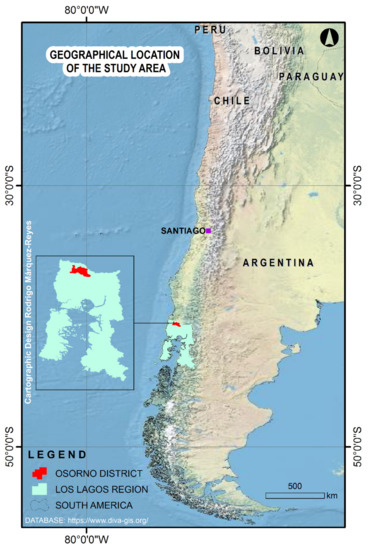
Figure 1.
Geographical location of the study area. Bar, 500 km.
The leading cause of air pollution in south-central Chile is considered to be the burning of firewood, used as a primary source of energy. It is reported that 96.3% of the population in Osorno uses firewood as a primary energy source for heating and cooking [2]. Many respiratory and cardiovascular diseases in Chile are related to wood burning, which emits PM [5]. In cities where wood smoke is the leading cause of air pollution, positive correlations between ambient particulate levels and mortality, hospital admissions, and acute respiratory infections for cardiovascular and respiratory diseases have been observed [6,7,8]. Moreover, several human epidemiological studies have found a consistent, strong relationship between PM exposure and lung and cardiovascular diseases [9,10,11,12].
Previous studies in Chile have investigated the correlation between PM2.5 and meteorological factors [13]. However, many studies have proven that the correlations between PM2.5 and meteorological factors vary with seasons and regions [14,15,16]. This study aims to clarify the source of PM2.5 in Osorno city by comprehensively analyzing the chemical compositions of PM2.5 and evaluating them in relation to meteorological conditions during part of the autumn–winter period of April to August. Furthermore, we attempt to provide information about the source and type of PM2.5 emissions and specific meteorological conditions.
2. Materials and Methods
2.1. Aerosol Samples
Aerosol samples were collected at the experimental monitoring station Emprender-ULagos, located at Colegio Emprender, Osorno (Figure 2 purple spot; latitude: 40°34′25″ S, longitude: 73°9′54″ W, altitude: 95 m) during April 2019–August 2019. Osorno city has an average altitude of 46.7 m above sea level (m.a.s.l.). It has a flat system of river terraces of 941.82 ha, with altitudes between 10 and 40 m.a.s.l., representing 64% of the inhabited and built surface of the urban system. Osorno is also characterized by a steep hill system towards the west, north, and southwest, with altitudes between 40 and 100 m.a.s.l.—equivalent to 527.84 ha—representing the remaining 36% of the built urban area. This detailed set of urban topographic characteristics constitutes an important factor for the circulation of winds within the city, and there is an approximately 73 m difference between the lowest and the highest points of the city.
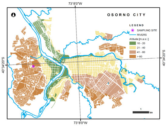
Figure 2.
A map showing the city of Osorno and the sampling site, Colegio Emprender Osorno. Bar, 1 km.
Airborne PM2.5 was collected employing a continuous particulate monitor BAM 1020 (Met One Instruments Inc., Grants Pass, OR, USA), which automatically collects and measures the PM2.5 using beta ray attenuation, designated to a U.S. EPA Federal Equivalent Method [17]. Beta attenuation monitoring (BAM) is a widely used air monitoring technique employing the absorption of beta radiation by solid particles extracted from airflow.
Met One BAM1020 Filter Tape P/N 460180 (LOT No. A25349276; Met One Instruments Inc., Grants Pass, OR, USA) glass fiber filter rolls were used. Airflow was 16.7 L/min and the monitor constantly collected samples at one spot per hour, collecting 24 spot samples per day. In more detail, the count time on the BAM 1020 was set to 8 min for a PM2.5 beta attenuation measurement; it performs the 8 min beta attenuation monitoring at the beginning and the end of each hour, with a 42 min air sample period (701.4 L/h) in between, for a total of 58 min. The other two minutes of the hour are used for tape and nozzle movements during the cycle. Two filter rolls were used during the period of this investigation. The first filter roll collected samples from 31 March 2019 to 15 June 2019, and the second filter roll collected from 15 June 2019 to 31 August 2019. For data validation, internal data files were used from the official air quality monitoring system of the Ministry of Environment, Chile. Additionally, the instrument performed a zero-filter test every six months (before and after the autumn–winter seasons). Additionally, 48–72 h valid 1-h data points were collected to determine the background. The initial zero-test allows us to determine the instrument noise and confirm the lower detection limit (LLD). For an 8-min count cycle, the manufacturer indicates that the LLD should be <4.8 µg/m3 for a 1-h measurement cycle and <1.0 µg/m3 for a 24-h measurement cycle. If the LDD is exceeded, the equipment is subject to maintenance by the brand’s authorized technical service (SETEC Ltda., Santiago, Chile). The uncertainty of the measurement results is 16% [18]. BAM 1020 operators do routine tasks to ensure data output quality, in conformance with the BAM 1020 operator’s manual. Data validation is carried out by means of correlation analysis with the official PM2.5 monitoring station of the Ministry of Environment, El Alba–Osorno, which compiles the methodology guidance defined by the primary environmental quality standard for fine respirable particulate material PM2.5 (Decree 12/2011, Ministry of Environment, Chile), and by the regulation of stations for the measurement of atmospheric pollutants (Decree 61/2008, Ministry of Health, Chile). Along with the PM2.5 concentration (μg/m3), meteorological parameters such as temperature (°C), barometric pressure (hPa), relative humidity (%), wind direction (°), and wind speed (m/s) were also measured at this station. Rain fall (mm) was measured using a Rika Weather Station RK600 (Hunan Rika Electronic Tech Co., Ltd. Hunan, China). The analysis utilized WRPlot ViewTM (Lakes Environmental Software. Waterloo, ON, USA).
Furthermore, ambient temperature and pressure mapping was generated with the dataset obtained by a Met One E-Sampler, a portable monitoring station (Met One Instruments Inc., Grants Pass, OR, USA). A total of 78 measurement points was selected and monitored for the thermal and atmospheric pressure analyses in Osorno city.
All times used in this study for measurements conducted in Osorno city were in Chilean standard local time (CLT).
2.2. PM2.5 Analyses
PM2.5 variation analysis and comparison of PM2.5 and meteorological data were conducted to find the relationship between PM2.5 and meteorological data and the seasonal variation in PM2.5 concentration.
The PM2.5 concentration variation analyses were conducted to observe any seasonal, monthly, or daily concentration variations.
2.3. Image J Analysis
Image J is an image analysis software that measures the area, mean, standard deviation, lengths, angles, and minimum/maximum of an image. Either an entire image or a selected image section can be used for this analysis [19]. Image J software was employed to analyze the relationship between black carbon and PM2.5 concentration in this study.
All the filter samples were digitized using a scanner, and the grayscale was analyzed with Image J. Then, by selecting the individual spots on the filter one by one—as shown in the red square in Figure 3—a total of 1837 spots were measured. Finally, the mean data of the measured spots were quantified by a gray color scale, and the corresponding PM2.5 concentration data obtained from the measuring site were compared with this data.
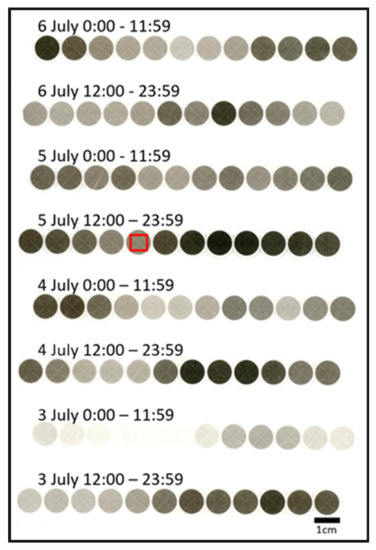
Figure 3.
An example of the filter samples used for the Image J analysis. The red square shows how the samples were measured and all the times are indicated in Chilean standard local time (CLT).
2.4. Cartography
Cartographies were designed and generated with an interpolative geostatistical procedure using ArcGis Desktop 10.5 software (Environmental Systems Research Institute, Inc., ESRI. Redlands, CA, USA. 2020)
2.5. Ion Chromatography Analyses
2.5.1. Sample Preparation and Ion Chromatography Settings
Six individual spots were combined as one sample to fulfill the minimum required concentration for the chemical analyses. Six spots were chosen per combined sample to see the daily variation.
Individual spots on the filter were cut into a 1 cm2 size and put together in a group of six in a 12 mL polypropylene PP-16L test tube (Maruemu Co., Osaka, Japan). Polypropylene test tubes were chosen instead of glass test tubes because, by using glass test tubes, the elements contained in the glass (Si, Al, and more) may contaminate the sample and affect the test results [20]. Then, 4 mL of deionized distilled water (DDW) generated by an Auto Still WG262 (Yamato Scientific Co. Ltd., Yamanashi, Japan) was added and sonicated with an Ultra Sonic Cleaner USK (AS ONE Co., Osaka, Japan) for 20 min at room temperature (ca. 25 °C). The solution was then filtered with a Minisart® Syringe Filter, Pore Size 0.45 µm (Sartorius AG, Göttingen, Germany) and a 5 mL Terumo syringe (Terumo Co., Yamanashi, Japan) for excluding the core fractions of particulate matters.
The obtained data were then analyzed using ion chromatography. Anions (F−, Cl−, NO2−, Br−, NO3−, PO43−, and SO42−) were measured with IC-20 (Dionex Co., Sunnyvale, CA, USA) using an IonPac AS12A column (Thermo Fisher Scientific Co., Waltham, MA, USA) and an AERS 500 suppressor (Thermo Fisher Scientific Co., Waltham, MA, USA). The eluent was 2.7 mM Na2CO3 and 0.3 mM NaHCO3. The column oven temperature was 30 °C. A total of 25 µL of the extracted sample was injected, and the flow rate was 1.5 mL/min. The standard solution used for the anions was prepared using a multi-anion standard solution (Br−: 100 mg/l, Cl−: 20 mg/l, F−: 20 mg/l, NO2−: 100 mg/L, NO3−: 100 mg/L, PO43−: 200 mg/L, SO42-: 100 mg/L in H2O) purchased from FUJIFILM Wako Pure Chemical Co. (Osaka, Japan).
Cations (Li+, Na+, NH4+, Mg2+, Ca2+, and K+) were measured with IC-2010 (Tosoh Co. Tokyo, Japan) using a TSKgel Super IC–CR column (Tosoh Co. Tokyo, Japan), and a suppressor TSKgel suppress IC–C (Tosoh Co. Tokyo, Japan). The eluent was 2.2 mM methanesulfonic acid and 1.0 mM 18-crown-6 ether. The column oven temperature was 45 °C. A total of 30 µL of the extracted sample was injected, and the flow rate was 0.8 mL/min. The standard solution used for the positive ions was prepared using a multi-cation standard solution (Li+: 5 mg/L, Na+: 20 mg/L, NH4+: 25 mg/L, K+: 50 mg/L, Mg2+: 30 mg/L, Ca2+: 50 mg/L in 0.02 mol/L HNO3) purchased from FUJIFILM Wako Pure Chemical Co. (Osaka, Japan). Four concentration levels of working calibration standard solution for calibration curves were prepared by diluting the multi-standard solution. A good linear correlation was found, with a coefficient of determination higher than 0.995 for anions and 0.997 for cations. The method detection limits (MDL) for the ion chromatography for the solutions of anions and cations ranged from 0.012 mg/L for F− to 0.12 mg/L for PO43−, and from 0.007 mg/L for Na+ to 0.027 mg/L for K+. The estimated uncertainties of the detected ions in this study from the linear calibration curve were in the ranges of 2% for SO42− to 8% for Ca2+.
From the ion chromatography measurement results, the two analyses described below were conducted.
2.5.2. Comparison of PM2.5 Concentration and Individual Ions
The individual ion concentrations for both cations and anions were compared with the total concentration of PM2.5 by a beta ray attenuation method. This comparison revealed the ions that showed high correlations with PM2.5 concentrations.
2.5.3. Correlation of Selected Ions
Selected ions were compared to identify the correlations between individual ions. Mainly, anions (F−, Cl−, NO2−, Br−, NO3−, PO43−, and SO42−), and cations (Li+, Na+, NH4+, Mg2+, Ca2+, and K+) were compared with Na+, Cl−, and K+, which were highly detected in the ion chromatography results. Out of all the compared ions, one of the top three ions that showed the highest correlation coefficient is shown in the result section. The correlation coefficient was calculated using the CORREL function in Microsoft Excel® (2013). For this study, the correlation coefficients were classified as follows: <0.29 (little if any correlation); 0.3–0.49 (low correlation); 0.5–0.69 (moderate correlation); >0.7 (high correlation) [21,22,23].
2.6. Backward Trajectory Analysis
The backward trajectory model NOAA HYSPLIT [24] was employed to obtain long distance air transport for the multi-component analysis. Three-day backward trajectories were conducted for both days with high PM2.5 concentrations (5 July 2019) and low PM2.5 concentrations (19 July 2019) to observe the differences in the air transport between days with both high and low PM2.5 concentrations. The highest selected was 0 m above ground level at the measurement site, Colegio Emprender, Osorno. The time used for the analyses was Coordinated Universal Time (UTC).
3. Results and Discussion
3.1. PM2.5 Analyses
3.1.1. PM2.5 Variation Analysis
This analysis was conducted to observe the daily variation in PM2.5 concentration using PM2.5 concentration data obtained from the sampling site. The daily variation analysis was conducted to determine the peak hours of PM2.5 pollution.
Figure 4 shows the daily variation in PM2.5 concentration. The PM2.5 concentration value showed large peaks between 19:00 and 23:00 (CLT), and two small peaks between 7:00 and 12:00 (CLT). These peaks occurred during the period in which many home activities are carried out by the local people. The peaks between 07:00 and 12:00 (CLT) may be due to meal preparation before school and work activities. The marked PM2.5 emissions increase at 19:00 (CLT) could be due to people returning from school and work to homes, increasing the demand for heating, along with various activities. In the last peak, at around 23:00 (CLT), the operation of heating devices to maintain comfortable temperatures in each household resulted in more emissions from wood burning, to keep the house heated at night. Furthermore, partially closing the draft hoods on heating equipment slows down the generation of heat, which contributes to incomplete combustion of the wood. This increasing trend in PM2.5 concentration at night can be seen in the top five highest PM2.5 concentration days. This result, showing two peaks in the morning and at night, is similar to the results obtained in densely populated New York and Beijing—both PM-polluted cities [16,25]. Many Chilean people use wood-burning devices for heating and/or cooking; these devices emit fine and coarse particles that contain toxic atmospheric pollutants [15].
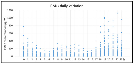
Figure 4.
Daily variation in PM2.5 concentration from April 2019 to August 2019.
3.1.2. PM2.5 and Meteorological Factors
The previous study reported that temperature, relative humidity, and wind speed influenced air pollutant concentrations [15,26]. In order to examine similar trends in Osorno, 6-h average meteorological data were compared with PM2.5 concentrations.
Figure 5a shows the relationship between PM2.5 concentration and temperature. The high PM2.5 concentration events are often seen at air temperatures between 5 and 10 °C. With the start of morning activities, increased emission of PM2.5 was associated with the anticipated use of wood-burning stoves for heating. The periods with temperatures below 5 °C did not show higher PM2.5 concentrations; a possible explanation is that the lowest temperature hours often occur in the early morning, when people are asleep and activities are limited. This idea accords with Figure 4, where at around 07:00 (CLT) the PM2.5 concentration starts to increase. Daily temperature variation in Osorno city reported by the Ministry of Environment showed that the early morning hours have the lowest temperatures of the day [27].
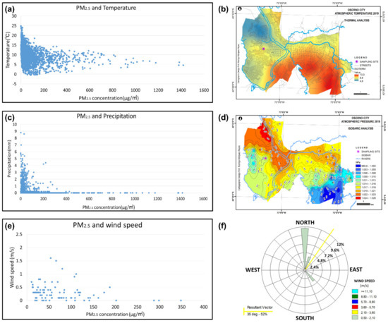
Figure 5.
Correlation between PM2.5 concentrations and some meteorological factors are indicated: (a) PM2.5 and temperature, (b) thermal analysis in Osorno city, (c) PM2.5 and precipitation, (d) atmospheric pressure of Osorno city with a color scale in hPa, (e) PM2.5 and daily average wind speed, and (f) wind rose in Osorno city during moderate air quality index days. Purple dots in (b,d) indicate the Emprender-ULagos air monitoring station sampling site, with the horizontal scale of the bar at 1 km.
Figure 5b shows the thermal analysis in Osorno city, including the emergency alert-level days of PM2.5 above 170 µg/m3 during fall–winter 2019. Low temperatures (ca. 4.3 °C) were predominant in the north and northwest part of the city, coinciding with the highest urban altitudes (ranging from 80 up to 122 m.a.s.l.). The second lowest temperatures (ca. 8.8 °C) were indicated in low altitude sections by the rivers; however, the ca. 40 to 60 m asl section in the south part of the city showed higher temperatures (ca. 13.3 °C). During the cold period, thermal inversions layers can form due to surface cooling, which prevents the air from mixing and promotes heavy air pollution episodes [25,26,28,29,30]. Additionally, at lower temperatures, increased emissions are associated with the combustion of firewood for heating [31,32,33]. Since meteorological conditions contribute greatly to thermal inversion layers, multiple factors, such as the thermal analyses done in this figure, must be conducted to prove heavy air pollution events. The highest temperature periods (ca. 13.3 °C) were observed in the south and southwest region of the city, on lands with altitudes ranging from 60 to 80 m.a.s.l (supplementary materials Video S1). The river basins showed an intermediate temperature profile during this period. Urban topography is a considerable factor in thermal variations recorded during April to September in different parts of the city, which increases the demand for firewood for heating.
Figure 5c shows the relationship between PM2.5 concentration and precipitation. The PM2.5 concentrations tended to be lower during precipitation events; this may be explained by the wash-out effect of the rain droplets [33]. In addition, it has been reported that a high concentration of PM2.5 is associated with changes in the vertical structure of clouds, which reduces the occurrence of local-scale precipitation [34,35,36,37], leading to less precipitation. The relationship between air pollution and precipitation is complex. Therefore, the obtained data should be considered one aspect of the PM2.5 concentration and precipitation relationship.
Figure 5d shows the atmospheric pressure mapping generated through 78 measurement points taken with an E-Sampler in Osorno city during fall–winter 2019. This figure shows a high correlation with Figure 5b. High-pressure domains were in the north, northwest, and northeast areas of the city (warm colors). From these areas, the displacement of urban air masses took place towards the southern and eastern areas, with lower barometric pressures (cold colors). The warm wind blowing from the north to the south indicates that wind brings PM pollution to the southern region.
Figure 5e shows the relationship between PM2.5 concentration and wind speed. This figure was based on the daily average instead of the six-hour averages of the other figures. As the wind speeds decreased, the PM2.5 concentration increased. Therefore, the dispersion of PM2.5 by strong winds is the most likely explanation. Additionally, these data indicate that the source of the PM was near the measurement station, which implies that Osorno city is the source of the PM2.5. Since Osorno city is located between Los Andes and the coastal mountains, episodic meteorological conditions produce poor ventilation in the valleys, and emissions due to anthropogenic activities [26,28,29,38,39]. Stagnant wind conditions allow air pollutants to accumulate, resulting in elevated and localized concentrations of air pollutants [16]. The topography influences PM2.5 concentrations even at the within-city level [40].
Figure 5f shows that the wind rose, indicating the wind speed and direction at the sampling site. The average wind speed was 0.32 m/s, with a calm wind frequency of 46.43%, resultant vector 20° (47%). Degrees (°) represent the origin of the wind, i.e., 0°, blowing from the north direction. Data were obtained from 3702 h of recording and 61.88% data availability. It can be seen that most of the particles came from 0–120° of the sampling site, indicating that the wind within Osorno city blows mainly from the north to the south, bringing PM to the sampling site. Since the wind continues to blow further south, it is important to establish a monitoring station to obtain data (supplementary materials Figure S1). Furthermore, the southwest region of the city has higher cases of respiratory infectious diseases; this area requires additional attention. Although there is some evidence to correlate respiratory infectious diseases and air pollution levels [41,42], it is important to monitor PM and other meteorological parameters in this southwest region.
Figure 6 shows the relationship between Chilean air quality indexes (depending on PM2.5 ranges) and meteorological parameters. Critical episodes of pollution, in both pre-emergency (red triangles) and emergency (purple diamonds) indexes, are inversely related to the minimum temperatures of the day—as Figure 6A shows; in the same way, and as was mentioned before, critical episodes of air pollution are associated with the lowest wind speeds and the absence of rain, as depicted in Figure 6B,C, respectively. Table 1 summarizes the meteorological data, according to the different air quality indexes (depicted in different colors).
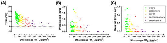
Figure 6.
Relationships between PM2.5, colored according to the Chilean air quality indexes defined by the Ministry of Environment, and meteorological factors. (A) the lowest (minimum) temperature of the day, (B) daily average wind speed, and (C) rain fall in 24 h.

Table 1.
Summary of meteorological data, according to the air quality indexes defined by the Chilean Ministry of Environment (Min. Environ).
3.2. Image J Analysis
In Figure 7, the PM2.5 concentrations increase exponentially as the grayscale values decrease. This figure shows the grayscale analysis results. A lower grayscale mean value indicates a darker filter color, and a higher grayscale mean value indicates a lighter filter color. A smaller grayscale mean value indicates lots of darker PM, suspected to be soot or rich in black carbon-containing pollutants, in the filter.
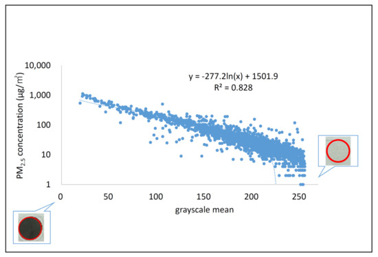
Figure 7.
Image J analysis of grayscale mean value and PM2,5 concentration plot for each sampling spot. The left bottom image in the balloon is a dark-colored PM2.5 sampling spot that indicates a small number of grayscale mean values, and the right gray-colored spot image of the right balloon image has higher grayscale mean values.
There are two possible reasons for this result. First, the filter color does not become darker after a certain level because the PM derived from biomass burning may have greater grayscale values with a lighter color, which does not show a correlation after a specific level of PM concentration. Second, the design of the sampling device may allow PM to accumulate in a focused spot, where a three-dimensional accumulation of PM2.5 occurs. This pile-up effect of PM2.5 on the filter surface, depositing PM2.5 particles on top of each other perpendicular to the filter surface, may decrease the Image J values.
This non-linear relationship with values less than 100 may suggest that the leading cause of PM2.5 emissions is not fossil fuel-related combustion, which often emits large amounts of soot and contributes to the darkness of the filter, showing high correlations with the PM2.5 concentration [43]. Since it is said that 96% of the population in Osorno uses firewood as a primary energy source [2], the non-linear relationship between the grayscale mean and PM2.5 concentration over and under 100 seen in Figure 7 may indicate a large contribution of PM2.5 from the incomplete combustion of firewood. It is said that soot is formed from the incomplete combustion of biomass and conventional fossil fuels [44]. However, it is suggested that increasing the combustion temperature promotes soot aggregation and generates more mature primary particles [45]. Therefore, firewood that burns at relatively low temperatures, compared to the internal combustion of fossil fuels, generates particulate matter with less oxidized incomplete substances than soot with relatively higher grayscale values. In Osorno, many households use fuels other than wood, i.e., various wastes, for burning, so this may lower the temperature and become a part of the reason for the incomplete combustion of wood.
3.3. Ion Chromatography Analysis
3.3.1. Comparison of PM2.5 Concentration and Individual Ions
Figure 8a shows the monthly variation in PM2.5 concentration. Data for 19 May–23 May 2019 was not obtained due to the malfunction of the beta ray attenuation unit for PM2.5 measurements. However, the filter rolls collected PM during this period despite the malfunction, so the individual ion data has no deficiencies.
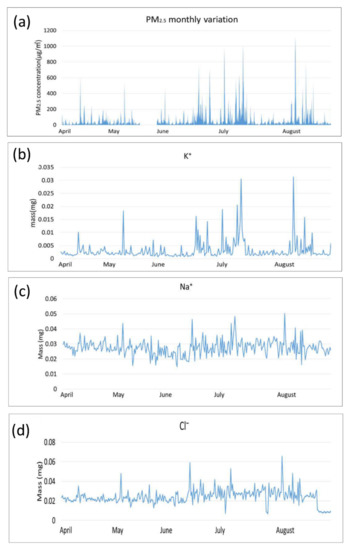
Figure 8.
April 2019 to August 2019 (part of autumn–winter) monthly variation in (a) PM2.5 concentration, (b) K+ concentration, (c) Na+ concentration, and (d) Cl− concentration.
The top five highest concentrations of PM2.5 were observed at 22:00 CLT on 2 August 2019 (1124 µg/m3), at 19:00 CLT on 5 July 2019 (1014 µg/m3), at 23:00 CLT on 30 June 2019 (982 µg/m3), at 23:00 CLT on 2 August 2019 23:00 (965 µg/m3), and at 21:00 CLT at 2 August 2019 (920 µg/m3) [26]. This observation is consistent with the data reported by the official monitoring station of the Ministry of Environment in El Alba, located in the central area of Osorno. The PM2.5 values were higher than 1000 µg/m3 during July 2019. Additionally, June and July showed the highest winter PM2.5 averages. From these data, it can be said that the winter season (June–August), on days with low temperatures, low wind speed, and little precipitation, had the highest PM2.5 concentrations for the experimental period of five months.
Figure 8 shows a clear similarity between (a) and (b), i.e., PM2.5 and K+ concentrations. However, there are no similarities between PM2.5 and Na+ and Cl−, as indicated in Figure 8a,c and Figure 8a,d. K+ is an index of biomass combustion, such as that with firewood [46,47]. This result indicates that biomass combustion with K+ as an indicator has a large impact on the PM2.5 pollution in Osorno.
3.3.2. Correlation of Selected Ions
Anions F−, Cl−, NO3−, and SO42−, and cations Na+, NH4+, Mg2+, Ca2+, and K+, which were highly detected in the 3.3.1 ion chromatography results, were compared with each other. Out of the 81 analyses, Na+ and K+, and K+ and F− showed moderate correlation coefficients of 0.67, respectively (Table 2, Figures S2 and S3). The highest correlation coefficient value of 0.93 was observed with PM2.5 and K+, indicating a strong connection between PM2.5 concentration and biomass burning.
Table 2.
The correlation matrix between ions and PM2.5. The bold font indicates the highest correlation coefficient value.
Figure 9 indicates a correlation of Cl− and Na+ with the coefficient value of 0.62. No adjustments have been made to the outlying data. Outlying data at the bottom section had a low Cl− concentration, below 0.1 mg/L. These sample spots were extracted and compared with meteorological data sets. From Table 3, these low Cl− concentration cluster spots had an average RH of 91(±9)%, but 15 out of 23 points indicated 0 mm precipitation, and the rest of the 8 spots had 0.6 to 1.9 mm of precipitation. Additionally, those spots showed an average wind speed of 0.25(±0.25) m/s, indicating a possible scenario of foggy days with low wind speeds. Such weather conditions allow Cl− to escape from the PM more readily, forming the low Cl− cluster. This phenomenon has been observed for a few decades, yet the detailed mechanism is still not fully understood [48,49,50]. This trend was also seen in Ca2+–Cl−, and Mg2+–Na+ from the same dates. Cl− can also be emitted from biomass burning [51,52]. In addition, a part of the NO3− replaces Cl− in NaCl to produce NaNO3. The presence of NO3− and Na+ in a certain ratio may produce NaNO3; further oxidation of NOX may generate NO3− ions through an oxidation process, which then replace the Cl− ions.
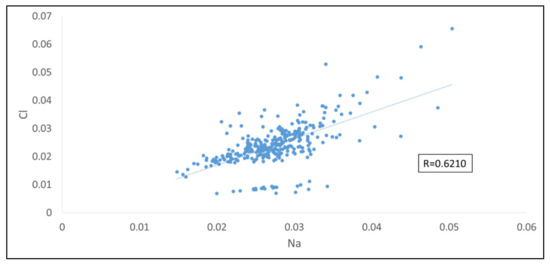
Figure 9.
Relationship between the detected ions; Na+ and Cl−.
Table 3.
Selective or faster removal process data for Figure 8. The data shown are 6-h averages. (Data for August 31 are 4-h averages).
3.4. Backward Trajectory Analysis
A backward trajectory analysis was conducted to simulate the air mass movement into Osorno. Figure 10a shows 5 July 2019 with a high PM2.5 concentration, and Figure 10b shows 19 July 2019 with a low PM2.5 concentration. The backward trajectory analyses conducted for both days with high and low PM2.5 concentrations showed a clear trend in the air mass movement into Osorno city from the South Pacific Ocean. These trajectory results suggest that marine aerosols may contribute to the PM2.5 in Osorno as a continuous input. A portion of the water-soluble ions in PM2.5 contain some marine-origin particulate matter; however, the total amount is somewhat limited. Thus, the marine-originated particulate matter is considered a limited base component of PM2.5 in Osorno city. Na+ is an ion also derived from biomass burning, so it is important to understand that the marine-derived Na+ is not the only source of Na+ detected from PM, since it is difficult to distinguish one from another. As mentioned above, Osorno city receives air mass from the South Pacific Ocean, and it is important to consider the effects of marine environment-derived Na+ or Cl−, as it may affect data interpretation.
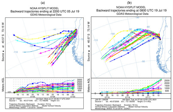
Figure 10.
(a) 5 July 2019 with a high PM2.5 concentration and (b) 19 July 2019 with a low PM2.5 concentration.
4. Conclusions
In this investigation, a strong correlation factor of 0.93 was found between PM2.5 concentration and K+. This result indicates that the monitoring of K+ can be employed as an index of biomass combustion, which is a leading cause of the high PM2.5 concentration in Osorno city. Additionally, the topographical features of Osorno city cause the thermal inversion layers to occur and cause increased concentrations of PM2.5.
A moderate correlation was found among the detected ions in PM2.5, which are often found in marine aerosols. This finding accords with the relatively low mountains on the west side of Osorno, allowing the air mass to reach the city and explaining the results of the backward trajectory analyses, showing a prevailing air mass movement from the South Pacific Ocean. However, the moderate correlation of marine-origin ions detected shows the difficulty of assessing the contribution of marine-origin PM2.5 in Osorno city. More importantly, the aforementioned PM2.5, which is generated from biomass burning combustion and from the thermal inversion layer caused by the topographical features of the Osorno city, contributed to high PM2.5 concentrations—reaching an emergency level of 1124 µg/m3. Therefore, continuous monitoring and mitigation strategies focusing on wood combustion activities are necessary to alleviate the current air pollution problem in Osorno city.
Supplementary Materials
The following are available online at https://www.mdpi.com/article/10.3390/atmos13020168/s1, Video S1: a video image of the emergency day of the winter period of Osorno city, an example from 18 July 2021; Figure S1: Wind rose separated by AQI; Figure S2: (a) NH4+ monthly variation, (b) Mg2+ monthly variation, (c) Ca2+ monthly variation, (d) F− monthly variation, (e) NO3− monthly variation, (f) SO42- monthly variation; Figure S3: Relationship between two detected ions. (a) Na+ and K+, (b) K+ and F-, (c) Na+ and NO2.
Author Contributions
Conceptualization, A.N., N.N., F.M., S.F., R.F., R.M.-R. and J.N.; methodology, N.N., F.M., S.F., R.F., R.M.-R. and J.N.; validation, A.N., N.N., F.M., S.F., R.F., R.M.-R. and J.N.; formal analysis, A.N., N.N., F.M., S.F., R.F., R.M.-R. and J.N.; investigation, A.N., N.N., F.M., S.F., R.F., R.M.-R. and J.N.; resources, N.N., F.M., S.F., R.F., R.M.-R. and J.N.; data curation, R.F. and R.M.-R.; writing—original draft preparation, A.N. and J.N.; writing—review and editing, N.N., F.M., S.F., R.F., R.M.-R. and J.N.; visualization, A.N., N.N., F.M., S.F., R.F., R.M.-R. and J.N.; supervision, J.N.; project administration, F.M.; funding acquisition, J.N., S.F., F.M., R.F. and R.M.-R. All authors have read and agreed to the published version of the manuscript.
Funding
This work was partly funded by FONIS SA17I0212 from the National Research and Development Agency (ANID, Chile) and DI R19/20 from Universidad de Los Lagos (to R.F. and R.M-R.); KAKENHI-PROJECT-19KK0263 to J.N., S.F. and F.M.
Acknowledgments
We would like to express our sincere gratitude to Hideyuki Otsuka (Hokkaido Research Organization), Motoomi Wakasugi (Hokkaido Research Organization), and Keiichi Tomita (Hokkaido Research Organization) for their generous support during the preliminary experiment and discussion of the selection of analytical method. Additionally, we would like to extend our appreciation for their technical support and medical record-related information to Carolina Moreira Alvarez and Romina Peña Flores, respectively. Additionally, we acknowledge the NOAA Air Resources Laboratory (ARL) for providing the HYSPLIT transport and dispersion model and/or READY website (https://www.ready.noaa.gov accessed on 15 December 2021) used in this publication.
Conflicts of Interest
The authors declare no conflict of interest.
References
- Instituto Nacional de Estadísticas. Censos de Población y Vivienda. Available online: https://www.ine.cl/ (accessed on 23 August 2021).
- Molina, C.; Toro, A.R.; Morales, S.R.G.; Manzano, C.; Leiva-Guzmán, M.A. Particulate matter in urban areas of south-central Chile exceeds air quality standards. Air Qual. Atmos. Health 2017, 10, 653–667. [Google Scholar] [CrossRef]
- World Health Organization (WHO). WHO Global Air Quality Guidelines: Particulate Matter (PM2.5 and PM10), Ozone, Nitrogen Dioxide, Sulfur Dioxide and Carbon Monoxide; World Health Organization: Geneva, Switzerland, 2021; Available online: https://apps.who.int/iris/handle/10665/345329 (accessed on 17 December 2021).
- Health Effects Institute. State of Global Air 2020; Data source: Global Burden of Disease Study 2019; Institute for Health Metrics and Evaluation: Seattle, WA, USA, 2020; Available online: https://www.stateofglobalair.org/data/#/health/plot (accessed on 15 October 2021).
- Garcia-Chevesich, P.A.; Alvarado, S.; Neary, D.G.; Valdes, R.; Valdes, J.; Aguirre, J.J.; Mena, M.; Pizarro, R.; Jofré, P.; Vera, M.; et al. Respiratory disease and particulate air pollution in Santiago Chile: Contribution of erosion particles from fine sediments. Environ. Pollut. 2014, 187, 202–205. [Google Scholar] [CrossRef]
- Sanhueza, P.A.; Torreblanca, M.A.; Diaz-Robles, L.A.; Schiappacasse, L.N.; Silva, M.P.; Astete, T.D. Particulate air pollution and health effects for cardiovascular and respiratory causes in Temuco, Chile: A wood-smoke polluted urban area. J. Air Waste Manag. Assoc. 2009, 59, 1481–1488. [Google Scholar] [CrossRef]
- Dominici, F.; Peng, R.D.; Bell, M.L.; Pham, L.; McDermott, A.; Zeger, S.L.; Samet, J.M. Fine particulate air pollution and hospital admission for cardiovascular and respiratory diseases. JAMA 2006, 295, 1127–1134. [Google Scholar] [CrossRef] [PubMed]
- Gan, W.Q.; FitzGerald, J.M.; Carlsten, C.; Sadatsafavi, M.; Brauer, M. Associations of ambient air pollution with chronic obstructive pulmonary disease hospitalization and mortality. Am. J. Respir. Crit. Care Med. 2013, 187, 721–727. [Google Scholar] [CrossRef] [PubMed]
- Krewski, D.; Burnett, R.; Jerrett, M.; Pope, C.A.; Rainham, D.; Calle, E.; Thurston, G.; Thun, M. Mortality and long-term exposure to ambient air pollution: Ongoing analyses based on the American Cancer Society cohort. J. Toxicol. Environ. Health 2005, 68, 1093–1109. [Google Scholar] [CrossRef] [PubMed]
- Pope, C.A., 3rd; Burnett, R.T.; Thurston, G.D.; Thun, M.J.; Calle, E.E.; Krewski, D.; Godleski, J.J. Cardiovascular mortality and long-term exposure to particulate air pollution- Epidemiological evidence of general pathophysiological pathways of disease. Circulation 2004, 109, 71–77. [Google Scholar] [CrossRef]
- Pope, C.A., 3rd; Burnett, R.T.; Thun, M.J.; Calle, E.E.; Krewski, D.; Ito, K.; Thurston, G.D. Lung cancer, cardiopulmonary mortality, and long-term exposure to fine particulate air pollution. JAMA 2002, 287, 1132–1141. [Google Scholar] [CrossRef]
- Rosenlund, M.; Berglind, N.; Pershagen, G.; Hallqvist, J.; Jonson, T.; Bellander, T. Long-term exposure to urban air pollution and myocardial infarction. Epidemiology 2006, 17, 383–390. [Google Scholar] [CrossRef]
- Koutrakis, P.; Sax, S.N.; Sarnat, J.A.; Coull, B.; Demokritou, P.; Demokritou, P.; Oyola, P.; Garcia, J.; Gramsch, E. Analysis of PM10, PM2.5, and PM2.5–10 concentrations in Santiago, Chile, from 1989 to 2001. J. Air Waste Manag. Assoc. 2005, 55, 342–351. [Google Scholar] [CrossRef]
- Yang, Q.; Yuan, Q.; Li, T.; Shen, H.; Zhang, L. The relationships between PM2.5 and meteorological factors in China: Seasonal and regional variations. Int. J. Environ. Res. Public Health 2017, 14, 1510. [Google Scholar] [CrossRef]
- Sánchez-Ccoyllo, O.R.; De Fátima Andrade, M. The influence of meteorological conditions on the behavior of pollutants concentrations in São Paulo, Brazil. Environ. Pollut. 2002, 116, 257–263. [Google Scholar] [CrossRef]
- DeGaetano, A.T.; Doherty, O.M. Temporal, spatial and meteorological variations in hourly PM2.5 concentration extremes in New York City. Atmos. Environ. 2004, 38, 1547–1558. [Google Scholar] [CrossRef]
- Met One Instruments. BAM 1020 Particulate Monitor Operation Manual; Met One Instruments: Grants Pass, OR, USA, 2016; Available online: https://metone.com/wp-content/uploads/2019/04/BAM-1020-9800-Manual-Rev-U.pdf (accessed on 17 August 2021).
- Hafkenscheid, T.L.; Vonk, J. Evaluation of Equivalence of the MetOne BAM-1020 for the Measurement of PM2.5 in Ambient Air; RIVM Letter Report 2014-0078; National Institute for Public Health and the Environment: Bilthoven, The Netherlands, 2014. [Google Scholar]
- Image, J. Image J Features. Available online: https://imagej.nih.gov/ij/features.html (accessed on 17 August 2021).
- Harrison, R.; Perry, R. Handbook of Air Pollution Analysis; Chapman and Hall: London, UK, 1986. [Google Scholar]
- Moore, D.S.; Notz, W.; Fligner, M.A. The Basic Practice of Statistics, 6th ed.; W.H. Freeman and Company: New York, NY, USA, 2011; Chapter 4. [Google Scholar]
- Asuero, A.G.; Sayago, A.; González, A.G. The correlation coefficient: An overview. Crit. Rev. Anal. Chem. 2007, 36, 41–59. [Google Scholar] [CrossRef]
- Westgard, Q.C. Z-12: Correlation and Simple Least Squares Regression. Available online: https://www.westgard.com/lesson42.htm#2 (accessed on 7 December 2021).
- National Oceanic and Atmospheric Administration (NOAA). Air Resources Laboratory. Available online: https://www.ready.noaa.gov/HYSPLIT.php (accessed on 17 August 2021).
- Liu, Z.; Hu, B.; Wang, L.; Wu, F.; Gao, W.; Wang, Y. Seasonal and diurnal variation in particulate matter (PM10 and PM2.5) at an urban site of Beijing: Analysis from a 9-year study. Environ. Sci. Pollut. Res. Int. 2015, 22, 627–642. [Google Scholar] [CrossRef]
- Mena-Carrasco, M.; Saide, P.; Delgado, R.; Hernandez, P.; Spak, S.; Molina, L.; Carmichael, G.; Jiang, X. Regional climate feedbacks in Central Chile and their effect on air quality episodes and meteorology. Urban Clim. 2014, 10, 771–781. [Google Scholar] [CrossRef]
- Sistema de Información Nacional de Calidad del Aire, Ministerio del Medio Ambiente. Available online: https://sinca.mma.gob.cl/index.php/estacion/index/key/A01 (accessed on 28 December 2021).
- Garreaud, R.D. The Andes climate and weather. Adv. Geosci. 2009, 22, 3–11. [Google Scholar] [CrossRef]
- Reizer, M.; Juda-Rezler, K. Explaining the high PM10 concentrations observed in Polish urban areas. Air Qual. Atmos. Health 2016, 9, 517–531. [Google Scholar] [CrossRef] [PubMed]
- Hussein, T.; Karppinen, A.; Kukkonen, J.; Härkönen, J.; Aalto, P.P.; Hämeri, K.; Kerminen, V.M.; Kulmala, M. Meteorological dependence of size-fractionated number concentrations of urban aerosol particles. Atmos. Environ. 2006, 40, 1427–1440. [Google Scholar] [CrossRef]
- Wiinikka, H.; Gebart, R. Critical parameters for particle emissions in small-scale fixed-bed combustion of wood pellets. Energy Fuels 2004, 18, 897–907. [Google Scholar] [CrossRef]
- Celis, J.E.; Morales, J.R.; Zaror, C.A.; Carvacho, O.F. Contaminación del aire atmosférico por material particulado en una ciudad intermedia: El Caso de Chillán (Chile). Inf. Tecnol. 2007, 18, 49–58. [Google Scholar] [CrossRef][Green Version]
- Ancelet, T.; Davy, P.K.; Trompetter, W.J.; Markwitz, A.; Weatherburn, D.C. Sources and transport of particulate matter on an hourly time-scale during the winter in a New Zealand urban valley. Urban Clim. 2014, 10, 644–655. [Google Scholar] [CrossRef]
- Guo, L.C.; Zhang, Y.; Lin, H.; Zeng, W.; Liu, T.; Xiao, J.; Rutherford, S.; You, J.; Ma, W. The washout effects of rainfall on atmospheric particulate pollution in two Chinese cities. Environ. Pollut. 2016, 215, 195–202. [Google Scholar] [CrossRef] [PubMed]
- Adler, G.; Flores, J.M.; Riziq, A.A.; Borrmann, S.; Rudich, Y. Chemical, physical, and optical evolution of biomass burning aerosols: A case study. Atmos. Chem. Phys. 2011, 11, 1491–1503. [Google Scholar] [CrossRef]
- Wall, C.; Zipser, E.; Liu, C. An investigation of the aerosol indirect effect on convective intensity using satellite observations. J. Atmos. Sci. 2014, 71, 430–447. [Google Scholar] [CrossRef]
- Chen, T.; Guo, J.; Li, Z.; Zhao, C.; Liu, H.; Cribb, M.; Wang, F.; He, J. A CloudSat perspective on the cloud climatology and its association with aerosol perturbation in the vertical over East China. J. Atmos. Sci. 2016, 73, 3599–3616. [Google Scholar] [CrossRef]
- Rutllant, J.; Garreaud, R. Meteorological air pollution potential for Santiago, Chile: Towards an objective episode forecasting. Environ. Monit. Assess. 1995, 34, 223–244. [Google Scholar] [CrossRef]
- Garreaud, R.D.; Rutllant, J.A.; Fuenzalida, H. Coastal lows along the subtropical west coast of South America: Mean structure and evolution. Mon. Weather Rev. 2002, 130, 75–88. [Google Scholar] [CrossRef]
- Peña, R. Prevalence Distribution of Chronic Obstructive Pulmonary Disease in the Commune of Osorno, Los Lagos Region, Chile in 2018. Master’s Thesis, Universidad Mayor, Santiago, Chile, 2020. (In Spanish). [Google Scholar]
- Wu, X.; Nethery, R.C.; Sabath, M.B.; Braun, D.; Dominici, F. Air pollution and COVID-19 mortality in the United States: Strengths and limitations of an ecological regression analysis. Sci Adv. 2020, 6, eabd4049. [Google Scholar] [CrossRef]
- Noda, J.; Tomizawa, S.; Takahashi, K.; Morimoto, K.; Mitarai, S. Air pollution and airborne infection with mycobacterial bioaerosols: A potential attribution of soot. Int. J. Environ. Sci. Technol. 2021, 19, 717–726. [Google Scholar] [CrossRef]
- Mansurov, Z.A. Soot Formation in Combustion Processes (Review). Combust. Explos. Shock Waves 2015, 41, 727. [Google Scholar] [CrossRef]
- Xi, J.; Yang, G.; Cai, J.; Gu, Z. A review of recent research results on soot: The formation of a kind of carbon-based material in flames. Front. Mater. 2021, 8, 695485. [Google Scholar] [CrossRef]
- Atiku, F.A.; Mitchell, E.J.S.; Lea-Langton, A.R.; Jones, J.M.; Williams, A.; Bartle, K.D. The impact of fuel properties on the composition of soot produced by the combustion of residential solid fuels in a domestic Stove. Fuel Process. Technol. 2016, 151, 117–125. [Google Scholar] [CrossRef]
- Clery, D.S.; Mason, P.E.; Rayner, C.M.; Jones, J.M. The effects of an additive on the release of potassium in biomass combustion. Fuel 2018, 214, 647–655. [Google Scholar] [CrossRef]
- Noda, J.; Bergström, B.; Kong, X.; Gustafsson, T.L.; Kovacevik, B.; Svane, M.; Pettersson, J.B.C. Aerosol from biomass combustion in Northern Europe: Influence of meteorological conditions and air mass history. Atmosphere 2019, 10, 789. [Google Scholar] [CrossRef]
- Finlayson-Pitts, B.J.; Pitts, J.N., Jr. Atmospheric Chemistry: Fundamentals and Experimental Techniques; John Wiley & Sons: New York, NY, USA, 1986. [Google Scholar]
- Abbatt, J.P.D.; Lee, A.K.Y.; Thornton, J.A. Quantifying trace gas uptake to tropospheric aerosol: Recent advances and remaining challenges. Chem. Soc. Rev. 2012, 41, 6555–6581. [Google Scholar] [CrossRef]
- Wang, X.; Jacob, D.J.; Eastham, S.D.; Sulprizio, M.P.; Zhu, L.; Chen, Q.; Alexander, B.; Sherwen, T.; Evans, M.J.; Lee, B.H.; et al. The role of chlorine in global tropospheric chemistry. Atmos. Chem. Phys. 2019, 19, 3981–4003. [Google Scholar] [CrossRef]
- Kundu, S.; Stone, E.A. Composition and sources of fine particulate matter across urban and rural sites in the Midwestern United States. Environ. Sci. Process. Impacts 2014, 16, 1360–1370. [Google Scholar] [CrossRef] [PubMed]
- McMeeking, G.R.; Kreidenweis, S.M.; Baker, S.; Carrico, C.M.; Chow, J.C.; Collett, J.L.; Hao, W.M.; Holden, A.S.; Kirchstetter, T.W.; Malm, W.C.; et al. Emissions of trace gases and aerosols during the open combustion of biomass in the laboratory. J. Geophys. Res. Atmos. 2009, 114, D19210. [Google Scholar] [CrossRef]


Publisher’s Note: MDPI stays neutral with regard to jurisdictional claims in published maps and institutional affiliations. |
© 2022 by the authors. Licensee MDPI, Basel, Switzerland. This article is an open access article distributed under the terms and conditions of the Creative Commons Attribution (CC BY) license (https://creativecommons.org/licenses/by/4.0/).