Climate Change Trends in a European Coastal Metropolitan Area: Rainfall, Temperature, and Extreme Events (1864–2021)

Abstract

This paper summarises an updated climate change trends analysis—developed for the period from 1 October 1864 to 30 September 2021 within the scope of a Horizon 2020-funded project to increase climate resilience in European coastal cities—for a representative site of the Lisbon Metropolitan Area (Portugal). By using long ground-based daily records of rainfall and surface temperature at the Lisboa-Geofísico climatological station, the analysis aimed to identify (i) long-term and recent climate trends in rainfall and temperature, (ii) changes in extreme rainfalls, heatwaves, and droughts, and (iii) possible effects of the coupled changes of minimum and maximum daily temperatures (Tmin and Tmax, respectively) on drought development based on the diurnal temperature range (DTR) indicator. To detect these trends and quantify their magnitude, the Mann−Kendall and Sen’s slope estimator tests were implemented. The analysis of the mean annual temperatures indicated that the study area has warmed ∼1.91 °C through the 157 analysed years. Results evidenced statistically significant upward trends in both Tmin and Tmax, and in the number of Tmax heatwave days. In what concerns the extreme hydrological events, the analysis of annual maximum rainfall series and peaks-over-threshold (POT) techniques showed more frequent and intense events in recent years, reaching up to ∼120.0 mm in a single day. With regard to drought, the study proved that the characterisation based on the commonly used standardised precipitation index (SPI) might differ from that based on the standardised precipitation evapotranspiration index (SPEI), as the latter can take into account not only rainfall but also temperature, an important trigger for the development of drought. According to the SPEI index, severe and extreme drought conditions have been more frequent in the last 60 years than in any other recorded period. Finally, a decreasing DTR trend towards the present was found to influence evapotranspiration rates and thus drought characteristics.

1. Introduction

Historically, coastal areas have been stressed by human activity, pollution, invasive species, and storms [1,2]. These environments could experience, on top of that, exacerbated impacts due to long-term shifts in temperatures and weather patterns [3,4]. Furthermore, among other things, climate change is likely to be detrimental to food and water security, particularly in coastal areas that are intensely urbanised. Warming temperatures and changes in rainfall regimes will affect the availability of energy and water, triggering regional tensions, also affecting international security welfare [5,6]. An increased frequency or magnitude of extreme hydrological events, heat and cold waves may adversely affect ecosystem health, and thus disrupt the stability of natural resources [7]. Moreover, the inherent uncertainty around climate impacts is likely to increase risks for other economic sectors.

Actions to tackle the aforementioned challenges should review, report and advance on the current state-of-the-art knowledge on changes in climate and their related impacts on natural resources in coastal urban environments [8]. To address such impacts, the very first thing that should be done is to identify and quantify trends over time of climate variables (e.g., annual rainfall, annual average maximum temperature) and their associated statistical and physical significance [9]. Analysing trends in rainfall and temperature is an important instrument for comprehending whether or not the climate is changing. The link between climate change and extreme events and some other features of the weather is still subject of debate. One of the major tools to support, or to reject, such links is trend analysis [10].

1.1. Trend Analysis of Climate Variables

Statistical trend estimation methods are well developed and include not only linear curves, but also change points, accelerated increases, other nonlinear behaviour, and non-parametric descriptions as summarised by Mudelsee [11]. Regarding climate, since the industrial revolution, humanity has exerted a significant impact on the climate, as evidenced by the increasing trend of global surface temperature (and of other climate variables such as annual rainfall, and annual number of heatwave days) against time since the 19th century [12,13,14]. Despite this fact being highly discussed among the public and researchers, it is, though, the use of statistics that give a number or quantify global warming. Statisticians have developed methods to quantify the warming trend and detect change points [15]. The most common types of error bars are standard deviation, standard deviation of the mean, and confidence interval [16]. Uncertainties are ubiquitous in all natural sciences, and error bars are an indispensable guide for the interpretation of any estimated trend analysis, for example, whether the Earth’s surface temperature did stop rising, stalling around the 2000s [17]. Therefore, to assess the accuracy of an estimation result, an uncertainty or statistically significant measure must be provided.

State-of-the-art, computing-intensive simulation algorithms take into account the peculiar aspects of climate data for trend analysis [18,19]. For some applications in Climate Research and Hydrology, for instance, relatively simple techniques such as moving averages or scatter diagrams can provide acceptable results [20]. However, where data are volatile, or where the early identification of turning points is critical, it is usually necessary to make use of more sophisticated mathematical techniques. Broadly speaking, trend estimation methods fall into parametric (or model-based) and non-parametric techniques [21]. In applications of statistics to climatology, such as the analysis of trends, parametric techniques are commonly utilised. Their correct use requires several assumptions to be fulfilled, including the type of distribution (most frequently normal), serial independence (i.e., zero autocorrelation), and stationarity. However, these assumptions are frequently violated by climatological data or are difficult to verify [21]. Alternatives include non-parametric (distribution-free) approaches, which ease up on assumptions about the nature of the problem. They tend to be more resistant to outliers than the parametric methods, but with a higher uncertainty in the statistical estimates [22].

1.2. Portuguese Vulnerability to Climate Impacts

In general, southern Europe is expected to experience an overall decrease in total rainfall, an increase in extreme rainfall events and a significant increase in the length of dry spells [23]. Portugal has a Mediterranean climate characterised by warm and dry summers and cool and wet winters [24]. The vulnerability of the country to recent climate variability has been well established [25]. Portugal has experienced a decrease in rainfall [26] and a rise in mean temperature accompanied by intensifying extremely high temperatures [27]. Furthermore, 8 of Portugal’s 10 warmest years on record have occurred in the last 20 years. The observations show a tendency towards more frequent and intense extreme weather events, in particular extreme rainfall, heatwaves, and droughts [24]. The Mediterranean region, and specifically Portugal, is regarded as a climate hotspot, which is projected to experience the greatest drying among 26 regions across the globe.

Vulnerability of Portugal to climate impacts is increasingly acknowledged in policy circles. During the European Council meeting in December 2019, President von der Leyen stated that “Portugal is one of the countries most affected by climate change” [28]. The Intergovernmental Panel on Climate Change (IPCC) has reported that southern Europe has experienced increases in temperature and decreases in rainfall because of climate change. Moreover, in the Mediterranean region, intensification of drought frequency and magnitude is projected to be substantially larger at 2.0 °C than at 1.5 °C of global warming. In Portugal, mean and extreme temperatures have increased in the past few years, with trends projected to be sustained well into the 21st century. Under a scenario where global warming reaches about 4.3 °C by 2100 (RCP8.5), maximum summer and autumn temperatures increase by up to 8 °C and maximum spring and winter temperatures increase between 2.0 °C and 4.0 °C with high confidence [29]. Under a scenario where global warming reaches about 3.0 °C by 2100 (RCP6.0), rainfall will decrease by about 30% in the southern part of Portugal and by about 15% in the northern part of the country with medium confidence [29]. However, the central western coastal areas (where the Lisbon Area is located) may differ from these projections.

Severe heatwaves, storms and droughts have already affected Portugal and will continue to do so, expectedly with increasing frequency and intensity. These impacts will have sectoral consequences. The Portuguese economy will also be affected as flows from tourism shift and climate-related hazards increase. The Portuguese wine industry is and will continue to be affected by climate change and olive trees are also at great risk. The Fifth Assessment Report (AR5) of the IPCC [30] states that climate projections show a marked increase with high confidence in high temperature extremes, meteorological droughts, and extreme rainfall events. Climate change is very likely to increase the frequency and intensity of heatwaves and other extreme weather events. The IPCC’s special report on the impacts of global warming of 1.5 °C [31] emphasises that limiting global warming to 1.5 °C is expected to substantially reduce the probability of extreme drought, rainfall deficits, and risks associated with water availability (i.e., water stress) in some regions. The IPCC’s special report on climate change and land [32] explains that frequency and intensity of droughts has increased in some regions including the Mediterranean and there has been an increase in the intensity of extreme rainfall events at a global scale.

The Lisbon Metropolitan Area is located at the mouth of Tagus river and a few kilometres away from the North Atlantic Ocean. It has been particularly recognised as vulnerable to the impacts of climate change [33]. Having a land morphology strongly impacted by the estuarine dynamics (e.g., storm surges and westerly winds) of the Tagus River and a fragile drainage infrastructure, the Lisbon Area is often impacted by both inland and estuarine flooding. The projected increase in storm surges also represents a threat to the environment. There is, furthermore, a high degree of confidence that flooding will increase and cause greater impacts and more severe damage to the metropolitan area by 2100 [33]. Moreover, on 18 February 2008, Lisbon experienced the rainiest day on record since 1876 with 118.40 mm [34]. This extreme event was responsible for a wide variety of negative impacts, namely urban inundations and flash flooding. Along with the extreme rainfall hazard, the Lisbon Area is greatly exposed to heatwaves [35], and droughts, according to recent trends and climate change prospects. Such claims make it relevant to analyse the trends of these climate variables and their impacts on the urban environment.

The previously mentioned issues have motivated the present climate change research, developed within the scope of the SCORE project (https://score-eu-project.eu/, accessed on 1 July 2022)—a Horizon 2020-funded research project to increase climate resilience in European coastal cities. For a representative Portuguese location of the Lisbon Metropolitan Area (including the City Halls of Lisbon, Oeiras, among others), the research was aimed at addressing (i) long-term and recent climate trends in rainfall in temperature, (ii) changes in extreme rainfalls, heatwaves, and droughts; and (iii) a discussion of possible effects of the coupled changes of minimum and maximum daily temperatures (Tmin and Tmax, respectively) on drought development.

Aside from this section, the paper is organised as follows: In Section 2, the case study, i.e., the Lisbon Metropolitan Area, is briefly mentioned along with the retrieved database. The used data refer to hydrological years (from 1 October of a given year to 30 September of the next year) including long daily records from the only climatological station in the metropolitan area, namely, of rainfall, minimum and maximum temperatures. For further analysis, the daily observations were aggregated into monthly and annual data. Section 3 describes the methods used in the study. The statistical models applied for trend analysis (the Mann–Kendall, Sen’s slope estimator, and Sequential Mann–Kendall trend tests), extreme selection methods (the peaks-over-threshold approach, standardised precipitation and evapotranspiration indices), and frequency analysis (the kernel occurrence rate estimator) are reported. Results regarding trends and frequency of rainfall and temperature, extreme rainfall, heatwaves, and droughts are presented in Section 4. In Section 5, the main findings are discussed with some additional insights to illustrate the climate change trends for the Lisbon Area. Section 6 gives some concluding remarks.

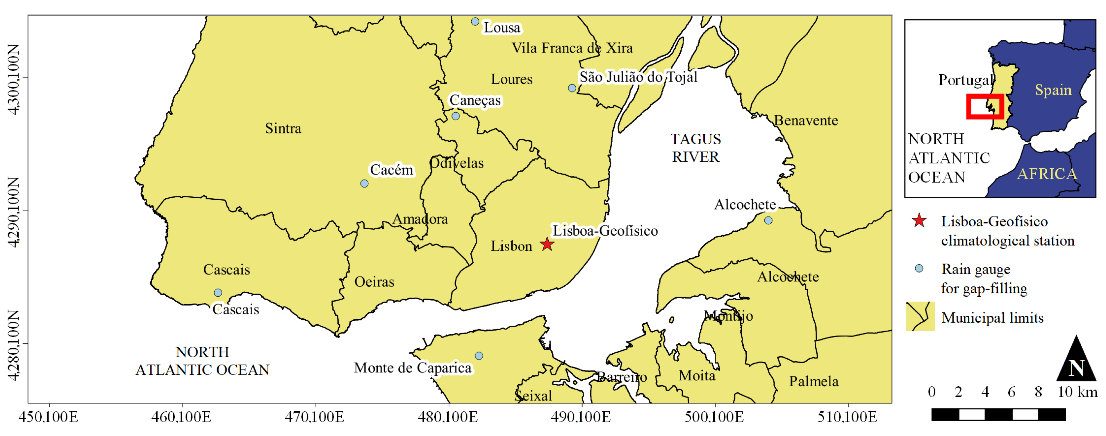
2. Study Area and Data Preparation

The Lisbon Metropolitan comprises a relatively small area (ca. 3000 km${}^2$) in which the capital of Portugal is located. Lisbon is the southwesternmost capital city in continental Europe, and the only one located on the North Atlantic coast—Figure 1. The metropolitan area (including the municipalities of Lisbon, Oeiras, among others) is the largest urban area in the country, with a population of 2,870,770 inhabitants in 2021 [36]. The coastal metropolitan area has a temperate climate, classified as Mediterranean, is characterised by dry and hot summers and wet and fresh winter periods.

The Lisboa-Geofísico climatological station (29U 487481.65 m E 4287553.88 m N, 77 m; Figure 1) was selected and assumed to be representative of the Lisbon Area as it is the only station in the region run by the Portuguese Met Office with long and high quality records of other variables besides rainfall. The Lisboa-Geofísico station is located at the first Meteorological Observatory in Portugal, the Infante D. Luiz Geophysical Institute (1853), providing a large amount of climatological and meteorological data compared to the limited and relatively short record length in surrounding stations [37]. The aim was retrieving the longest quasi–continuous daily rainfall and temperature series to create a comprehensive picture of climate and its changes in the Lisbon Metropolitan Area. Hence, daily records of rainfall, minimum (Tmin) and maximum (Tmax) temperatures at the Lisboa-Geofísico station were acquired from the Portuguese Institute for the Ocean and Atmosphere, IPMA (https://www.ipma.pt/en/, accessed on 1 July 2022) covering 157 hydrological years from 1 October 1864 to 30 September 2021—omitting leap year days for computational purposes. IPMA is the national authority in the fields of meteorology, aeronautical meteorology, climate, seismology and geomagnetism, and an institution of reference at the international level devoted to the promotion and coordination of scientific research. It has very high data quality standards and is considered the most reliable source of Portuguese hydrological and hydrometeorological data.

Despite the regular data maintenance in the databases at the Lisboa-Geofísico station, the retrieved rainfall series presented 130 missing daily records during the short subperiod from 1 January 2019 to 30 September 2019. For statistical reasons, valid climatic analyses require continuous, complete and long time series [38]. Therefore, the missing observations were filled via the multivariate, imputation by chained equations (MICE)—e.g., [39,40]. For gap-filling, the daily records at rain gauges in the vicinity of the Lisboa-Geofísico station (Figure 1) were retrieved from the Portuguese National Water Resources Information System website (https://snirh.apambiente.pt/, accessed on 1 July 2022). Overall, the MICE algorithm is a robust method to deal with missing data through an iterative series of predictive models [41,42]. After the gap-filling, a complete daily dataset from 1 October 1864 to 30 September 2021, including rainfall, was assembled. Thus, the core series of rainfall, Tmin and Tmax supporting the research were: daily, monthly, annual, and annual maximum daily (annual minimum daily for Tmin). Annual series are shown in Figure 2.

3. Methods

Long-term and recent climate trends were addressed based on the ground-based rainfall and surface temperature records (from 1864/65 to 2020/21) described in the previous section. This also included the analyses of changes in extreme rainfall, heatwaves and droughts by applying mainly non-parametric methods, here briefly described—mostly implemented in R Studio (https://cran.r-project.org/, accessed on 15 July 2022).

3.1. Non-Parametric Models for Monotonic Trends

The broadly-used rank-based non-parametric Mann–Kendall (MK) test [43] coupled with Sen’s slope estimator test [44] were applied to annual series of climate variables (assumed to have no autocorrelation in the studied period) to identify and quantify long-term monotonic trends. A positive (negative) Sen’s slope estimate can be interpreted as a monotonic upward (downward) trend meaning that the variable consistently increases (decreases) through time. A hypothesis is set as follows: $H_0$ null hypothesis signifies no trend. An alternative hypothesis, $H_1$, indicates the presence of trend, either increasing or decreasing monotonic trend. The probability associated with the standardised MK trend statistic, S, and the sample size n (here, $n=157$) is calculated to assess the significance of the trend. In this research, the significance level of $\alpha =0.05$ for a two-sided test was adopted. When testing upward or decreasing monotonic trends at the $\alpha$ significance level, $H_0$ is rejected for an absolute value of MK z greater than MK $z_{1-\alpha /2}$. For $\alpha =0.05$, MK $z_{1-0.05/2}$ is 1.96. The MK z values, or normalised test statistics, also show the significance of the trend where the negative and positive MK z values denote downward and upward trends, respectively. In addition, for the Sen’s slope estimates, if the p-value is less than the $\alpha$, $H_0$ is rejected, and the results are statistically significant.

To investigate the change in the trend of the selected variables with time, the sequential Mann–Kendall (SQMK) test was used [45]. To a large extent, the test makes use of progressive $u\left(t\right)$ and retrograde $u^{\prime }\left(t\right)$ sequential trend statistic series. In the data processing, the test compares the relative magnitudes of data instead of the data values directly. In this case, $u\left(t\right)$ and $u^{\prime }\left(t\right)$ are progressive and retrograde trend series, respectively, i.e., standardised variables (the Z-scores) that have a unit standard deviation and a zero mean. The $u\left(t\right)$ values were calculated using the MK test for each dataset, from the start to the end of the study period. Analogously, the $u^{\prime }\left(t\right)$ values were calculated backwards. In the plot of sequential MK, the confidence limits for a two-sided interval of the standard normal Z-scores were set at $\alpha =0.05$, that is, ±1.96. A significant trend is noted if the progressive MK values, i.e., $u\left(t\right)$ series, cross either of the previous limits.

3.2. Annual Maximum (AMAX), Annual Minimum (AMIN), and Partial Duration Series (PDS)

For analysing some extreme events of the selected climate variables at daily scale, the annual maximum series (AMAX), annual minimum series (AMIN), and the partial duration series (PDS)—also denoted the peaks-over-threshold (POT)—sampling techniques were utilised [46]. AMAX was applied to rainfall and Tmax; AMIN to Tmin; and POT to rainfall, in this last case, aiming at extracting only the dates (POT time data) of the extreme rainfall events—and not the magnitudes of those events (POT data)—to support the analysis of their frequency. The traditional AMAX, or AMIN, sampling method is still the most used one in hydrological extreme frequency analysis in many countries [47]. For each hydrological year, AMAX (AMIN) selects only the highest (lowest) value of the variable under consideration. In comparison with AMAX, POT sampling includes the values that are higher than a given threshold meeting the independence condition [48,49]. Accordingly, some events that are not AMAXs, but still relatively high, are included in the POT series, thus potentially improving the sampling of extremes.

Choosing the threshold, a, to be considered in the POT sampling is a subjective and major issue of the method as there is no universally accepted rule for that selection, as reviewed by Pan et al. [50]. Different thresholds result in different samples of both the peak magnitudes and their times of occurrence. On the one hand, too low thresholds might trigger the sampling of dependent peaks or peaks not corresponding to extreme events, and, on the other hand, too high thresholds lead to reduced sample sizes, compromising the advantage of the POT sampling comparatively to the AMAX one, in terms of sample length. Therefore, rather than considering a given threshold, values varying quasi-continuously of thresholds should be analysed and checked for their adequacy and independence of the POT data.

The exceedances above a given threshold generally occur in clusters (events), making it necessary to apply a declustering procedure to identify approximately independent cluster maxima. The independence criterion used in the present study selected the peaks belonging to rainfall events separated in time by at least one day without rainfall [51]. Only the maximum daily rainfall of each of the selected clusters were considered, together with the dates of such maximum rainfalls, i.e., the time data. For a given threshold and for the significance level $\alpha =0.05$, the independence of the POT data and the Poisson assumption of the POT time data were checked based on the lag-one and two autocorrelation coefficients [52] and on the dispersion index, respectively [50,53,54,55]. The dispersion index is the ratio between the variance and the mean of the POT time data sample, which takes values close to unity under the Poisson assumption. To evaluate the adequacy of the threshold, three plots were obtained as a function of variable thresholds [48,53,54], i.e., the mean annual number of over-threshold events, the mean exceedance above threshold, also known as mean residual life plot (MRL), and the dispersion index. For the selected threshold a, the adopted criteria considered that the:

• POT sampling technique should result in at least three peaks per year on average;
• MRL plot should be approximately linear for values including the threshold; confidence intervals, based on the normality assumption, were added to the plot;
• dispersion index should be located within the limits of the confidence interval given by a ${\chi }^2$ distribution with $n-1$ degrees of freedom, where n is the number of years of the recording period.

The significance level adopted in the last two points was $5\%$ (two-sided intervals).

3.3. Standardised Precipitation (SPI) and Evapotranspiration (SPEI) Indices

To detect droughts—here defined as sustained and regionally broad occurrences of below average natural water availability [56]—at the study area, the standardised precipitation index (SPI), developed by McKee et al. [57], was the first of two methods used. The SPI was applied to monthly rainfall at the Lisboa-Geofísico station to assess two different drought types and timescales, namely: (i) severe and extreme droughts for (ii) 6 and 12-month SPI, i.e., SPI6 and SPI12. The drought thresholds recommended by Agnew [58], namely, $u_{se}=-1.28$ for severe drought, and $u_{ex}=-1.65$ for extreme drought, were adopted. Shorter timescales of SPI were not considered since they usually are linked to water deficits and to the short-term change drought characteristics [59]. As the timescale increases, the response of SPI6 and SPI12 to short-term rainfall decelerates, resulting in more stable and well-defined droughts. Both the SPI6 and SPI12 better reflect long-term changes in river runoff, groundwater level and reservoir water storage capacity, for instance.

Given the critical role of temperature and hence evapotranspiration on drought development, the standardised precipitation evapotranspiration index (SPEI), an extension of the SPI [60], was also used for drought detection. The SPEI is designed to take into account both rainfall and potential evapotranspiration (PET) in identifying droughts. Going beyond the SPI, the SPEI captures the main impact of temperature changes on water availability. Like the SPI, the SPEI can be calculated on a range of timescales from 1 to 48 months. If only limited data are available, say temperature and rainfall—as it is the case of the present analysis—PET can be estimated with the simple Thornthwaite method based on mean temperature (Tmean) [61]. In the previous method, variables that can affect PET such as wind speed, surface humidity and solar radiation are not accounted here. The timescales and drought thresholds considered were the same as for the SPI, i.e., SPEI6 and SPEI12 for severe, $u_{se}=-1.28$, and extreme, $u_{ex}=-1.65$, droughts. Both the SPI and SPEI were calculated via the package ’SPEI’ implemented in R Studio by Beguería et al. [62].

3.4. Heatwave Magnitude Index

Prolonged periods of abnormally hot weather, i.e., heatwaves, were addressed from 1864 to 2021 based on the heatwave magnitude index according to Russo et al. [63]. The adopted heatwave magnitude index is defined as the maximum magnitude of the heat waves in a year, where heat wave is the period ≥3 consecutive days with Tmax above the daily threshold. The threshold is defined as the 90th percentile of daily Tmax, centred on a 31-day window. Hence, for a given day d, the threshold series $A_d$ of the dataset is given by

$$A_d=\bigcup _{y=1864}^{2021}\bigcup _{i=d-15}^{d+15}{T}_{y,i},$$

(1)

where ⋃ denotes the union of sets and $T_{y,i}$ is daily temperature, in this case Tmax, of the day i in the year y. To apply the previous equation, the daily records of Tmax in the 15-day period before 1 October 1864 and after 30 September 2021 were also retrieved.

3.5. Kernel Occurrence Rate Estimator for Extreme Events

The analysis of the changes in the frequency of occurrence of extreme events were addressed by applying a kernel occurrence rate estimator (KORE), according to the stepwise approach applied by Silva et al. [53] and Silva [64]. This included the generation of pseudodata outside of the observation interval, by the straightforward method of reflection for an amplitude of three times the bandwidth. The time data considered in the KORE related to: (i) extreme rainfall from the POT series, (ii) Tmax heatwave days, and (iii) the periods under drought conditions according to SPI and SPEI. As a result, the occurrences per year, $\lambda \left(t\right)$, of the extreme events were computed through the period from 1864 to 2021.

4. Results

Over the analysed period of 157 years, the Lisbon Metropolitan Area’s climate has apparently gone through some substantial changes. Aiming at providing a general characterisation of the assembled dataset and stressing some of those changes, subperiods of the reference period were analysed regarding rainfall and temperature. In line with World Meteorological Organization (WMO) guidelines [65], 30-year ’averaging’ periods were adopted to act as a benchmark against which the observational records can be compared in different contexts—Figure 3. The 30-year periods adopted in the figure emulate WMO climatological normals’ periods.

Figure 3 shows some fundamental attributes of the annual series of the analysed variables. As a measure of central tendency, the 30-year averages and other statistics (e.g., the median and the mean) characterise the background state about which anomalous conditions and even extremes are allowed to operate [66]. These ’normals’ include three major products, each of them with two sub-products: rainfall-related (total and AMAX, Figure 3a,d), Tmin-related (average and AMIN, Figure 3b,e), and Tmax-related (average and AMAX, Figure 3c,f) normals.

The rainfall-related normals have mean values always higher than their respective median, which evidences that the data are right–skewed (Figure 3). In addition, the rainfall-related box-plots in the most recent period (from 1991/92 to 2020/21) have much longer whiskers compared with those of the first period—from 1871/72 to 1900/01. This represents a greater range for the overall sample and more interannual variability in rainfall recently. Regarding the Tmin-related normals, the latest numbers have risen comparatively with the previous period. Apparently, there is a generalised positive trend in the Tmax-related ’normals’ with warmer conditions lately. In summary, the values of the six variables have much higher values in the last two periods and increased over time with an apparent positive, or upward, trend. Nevertheless, at this point, the statistical significance of such behaviour is not yet clear.

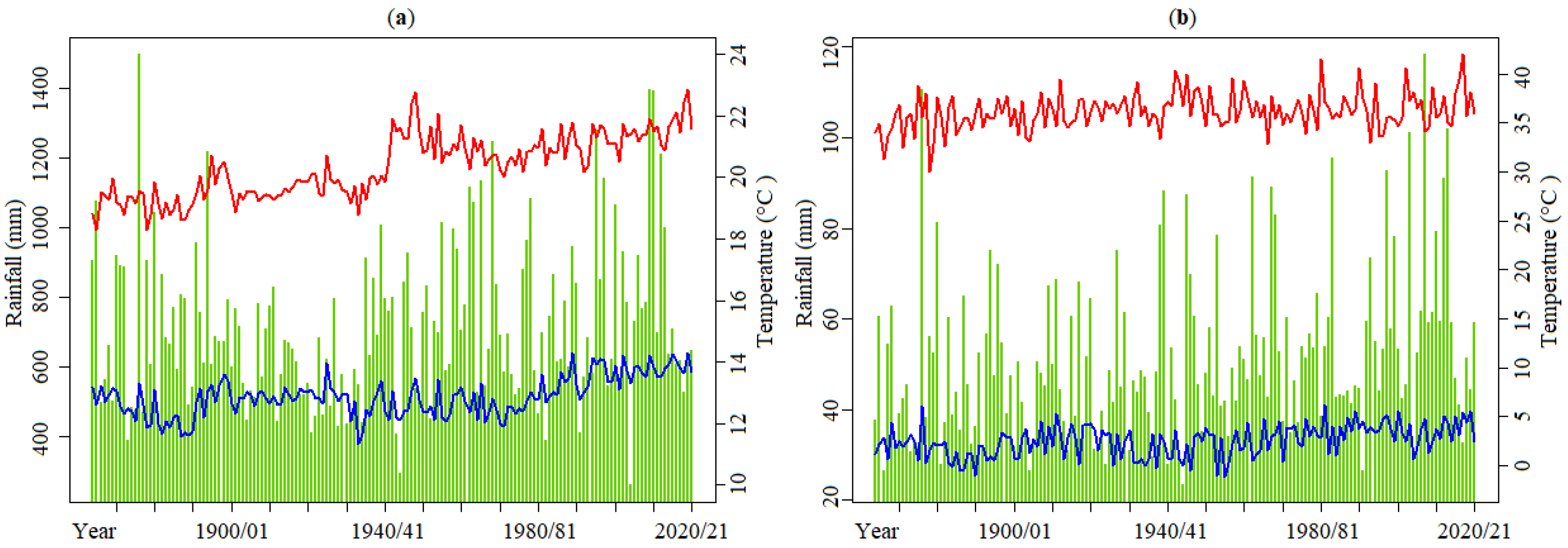
4.1. Trends of Climate Variables

As mentioned, the trend analysis at the Lisboa-Geofísico station was performed based on 157 hydrological years of rainfall, Tmax and Tmin data, from 1864/65 to 2020/21. The Mann–Kendall and Sen’s slope estimator tests were used to identify and quantify the magnitude of the linear trends of the annual series of Figure 3, i.e., rainfall, average Tmin and Tmax, maximum daily rainfall and Tmax, and minimum daily Tmin. The results achieved, including some statistics of the series, are outlined in

Table 1. Summary of statistics, Mann–Kendall test z, and Sen’s slope estimates (in units per year) related to the annual series of climate variables at the Lisboa-Geofísico station from 1864/65 to 2020/21 ($n=157$) at a significance level of $\alpha =5\%$.

Climate Variable	Unit	Minima	Maxima	Mean	MK z	p-Value	Slope
Rainfall	mm	260.90	1497.00	714.21	1.6423	0.1005	0.5966
Average Tmin	°C	11.30	14.30	12.88	6.0729	1.25 $\times {10}^{-9}$	0.0073
Average Tmax	°C	18.27	22.86	20.34	11.6560	2.2 $\times {10}^{-16}$	0.0180
Maximum daily rainfall	mm	23.30	118.40	51.48	3.3499	0.0008	0.0925
Minimum daily Tmin	°C	−1.20	6.20	2.50	5.0289	4.933 $\times {10}^{-7}$	0.0146
Maximum daily Tmax	°C	30.00	42.00	36.16	2.9655	0.0030	0.0097

.

As reported in the table, annual rainfall shows great variability, ranging from 260.90 (in 2004/05) to 1497.00 mm (in 1876/77). A non-significant trend (MK $z<$ 1.96, and p-value $>0.05$) in annual rainfall was observed with a total increment of 93.67 mm in 157 years. In contrast, AMAX daily rainfall denoted a significant trend (MK $z>1.96$, and p-value $<0.05$) with an increase of 14.53 mm in the reference period. The annual average temperatures denoted significant trends with increases of 1.2 °C for Tmin and 2.8 °C for Tmax in 157 years—both increments are beyond the long-term natural variability, with much higher values than the standard deviation (${\sigma }_x$) of their respective annual average series (${\sigma }_x=0.64$ °C for Tmin, and ${\sigma }_x=1.00$ °C for Tmax). The same response with significant results was detected regarding AMIN daily Tmin and AMAX daily Tmax with upward trends within the studied years (2.30 °C and 1.52 °C, respectively), which were also greater than their standard deviations (${\sigma }_x=1.64$ °C for AMIN daily Tmin, and ${\sigma }_x=1.91$ °C for AMAX daily Tmax).

As a summary of the previous results, it can be said that, except for the non-statistically significant trends of the annual rainfall, the analysed climate variables denoted significant upward trends, a pattern that is in line with the long-term global trends and those for the Mediterranean, Western and Central Europe [67]. For a better understanding of the previous results, the sequential Mann–Kendall (SQMK) test was applied to plot the development of the trends based on the Z-scores for the climate variables of Table 1.

Figure 4 depicts yearly plots of $u\left(t\right)$ and $u^{\prime }\left(t\right)$ values for each of the variables. As for the climate variables with significant trends, the $u\left(t\right)$ of the annual average of Tmin and Tmax of Figure 4a showed almost parallel trends from the start of the reference period until the year 1940/41. From that year onward, the $u\left(t\right)$ trend series diverged—Tmax continuing with sustained upward trend, and Tmin shifting to a downward trend until 1980/81. From the late 1960s onward, the annual average Tmin $u\left(t\right)$ changed from negative to positive values, exceeding Z-score $=+1.96$, with a much faster rate compared to the annual average Tmax $u\left(t\right)$. As it can be seen in Figure 4b, a similar response was detected for the AMIN Tmin $u\left(t\right)$ although with high positive trends starting in the early 1960s. This also applied to the AMAX daily rainfall $u\left(t\right)$, i.e., sustained upward trends from the mid-1960s to the end of the reference period. Considering that the paired $u\left(t\right)$ and $u^{\prime }\left(t\right)$ series never intersected, significant change points in trends were not detected.

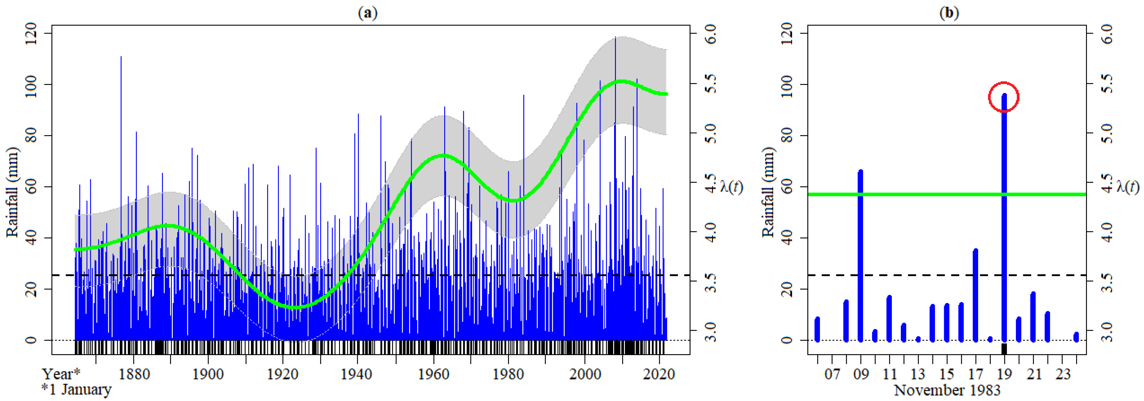
4.2. Peaks-over-Threshold (POT) Analysis of Extreme Daily Rainfall Frequency

Aiming at addressing the frequency of the extreme rainfall events, the POT sampling technique was applied to the daily rainfall data from 1 October 1864 to 30 September 2021. The criteria presented in Section 3.2 resulted in a threshold of $a=25$ mm. For this threshold, the correlation structure of the peaks or exceedances was analysed. Non-significant serial correlation was found (lag one and lag two autocorrelation coefficients of 0.074 and 0.022, respectively, i.e., within the 95% confidence intervals). Figure 5a–c show the results of the tests done to evaluate the adequacy of the threshold, based on plots as function of variable thresholds of the mean number of over-threshold peaks per year, the mean exceedance above threshold, and the dispersion index, respectively. For the selected threshold, the number of total exceedances (or peaks) was 665, i.e., 4.2 exceedances per year during the 157 studied years.

The kernel technique KORE was applied to the POT time data obtained from the daily rainfall time series aiming at estimating the extreme rainfall occurrence rate curve, $\lambda \left(t\right)$, that is, the number of independent extreme rainfall, or peaks-over-threshold, per year (Figure 6a). A point-wise bootstrap confidence band was constructed around $\lambda \left(t\right)$ for a more accurate interpretation of the results. The confidence band quantifies the uncertainties associated with the occurrence rate estimates: The narrower the band is, the less uncertainty. Overall, $\lambda \left(t\right)$ in Figure 6a shows an upward direction from the year 1920 to 1960, and thereafter a decade of lower occurrence rates. However, there was a direction change with steeper increase in $\lambda \left(t\right)$ from the late 1960s on, translated into more than five extreme rainfall events per year. By way of example, one of the extreme rainfall events from Figure 6a is depicted in Figure 6b. This event started on 8 November 1983, finished 14 days later, and was preceded and followed by days without rainfall, as required by the POT approach. The peak of the rainfall event had a magnitude of 95.60 mm on 19 November 1983—only this date was the input into the KORE model for such rainfall event. Note that the magnitude of peak-over-threshold events, as well of other extreme climate variables’ occurrences, were estimated but not thoroughly reported in this article.

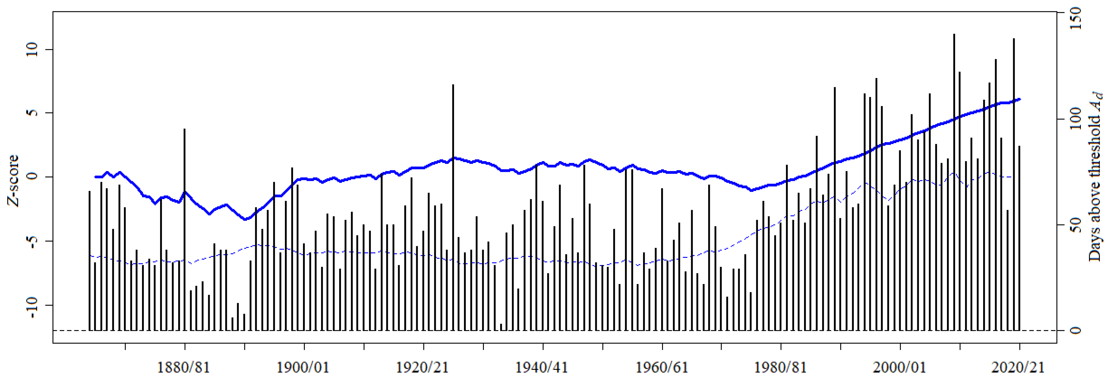
4.3. Heatwave Days of Tmax

By using the heatwave magnitude index, the threshold series $A_d$ was calculated for the period from 1 October 1864 to 30 September 2021—sinusoidal–type wave in Figure 7. This allowed identifying heatwave days in the daily Tmax series, i.e., three or more consecutive Tmax days above $A_d$. As a result, 9221 heatwave days out of the total analysed 57,305 days were identified, representing about 17% of the time. However, a closer look at the last 15 years highlights that 30% of the days have been heatwave days of Tmax (102 heatwave days per year). The latter straightforward figure was confirmed by the KORE applied to the time data of the Tmax heatwave days—i.e., the dates or time data of ≥3 consecutive days with Tmax above $A_d$, as presented in Figure 7a. The figure shows that the occurrence rates have changed over time. For example, the peak of $\lambda \left(t\right)$ from the year 1864 to 1970 is clearly lower than that of recent years with approximately 105 occurrences per year. In the same figure, the narrow confidence band around $\lambda \left(t\right)$ demonstrates a small uncertainty of the occurrence rate estimates. Given that the sinusoidal pattern of $A_d$ is almost imperceptible in Figure 7a, out of the 157 years, a detail for a 7-year period from the year 1975 to 1980 is presented in Figure 7b.

The previous increase in Tmax heatwave days was corroborated by the Sen’s slope estimator and SQMK tests. Figure 8 shows the SQMK results of number of Tmax heatwave days in each year. According to the models applied, there is a statistically significant upward trend (p-value=2.2 $\times {10}^{-16}$ < 0.05, Table 1) rising more rapidly from the year 1938/39 on. Additionally, no changing point was identified given that the paired $u\left(t\right)$ and $u^{\prime }\left(t\right)$ trend lines never cross each other. The total increase of Tmax heatwave days was 71 throughout 157 years. These results, coupled with those of the KORE analysis, highlight the fact that extreme Tmax conditions are becoming more common at the Lisboa-Geofísico station.

4.4. Temporal Evolution of Droughts

The standardised precipitation index (SPI) and the standardised precipitation evapotranspiration index (SPEI) were applied to monthly rainfall series (and to temperature series in the case of SPEI) to identify droughts in the Lisbon Area during the 157-year period (1884 monthly observations). These indices were coupled with the KORE approach for analysing the frequency of drought, i.e., the periods when SPI and SPEI drop below the adopted drought thresholds. Figure 9 shows the results for SPI at 6 and 12-month scales, i.e., for SPI6 and SPI12 (upper plots for severe droughts, lower ones for extreme droughts).

According to Figure 9a, in the first decades of the 20th century, the frequency or occurrence rate $\lambda \left(t\right)$ of drought built up, reaching a peak for both severe and extreme drought conditions around the year 1930. Following this, a trough was reached at the early 1960s with an apparent decreasing trend until the end of the period under analysis. In relation to the SPI12 series (Figure 9b), the same pattern of $\lambda \left(t\right)$ was detected, although only for severe drought conditions. In fact, Figure 9b shows that the frequency of the periods under extreme drought conditions has increased somewhat steadily throughout the studied period. Overall, the identified droughts had interannual and interdecadal changes with slight differences in the $\lambda \left(t\right)$ fluctuation and were more frequent in the past than in recent years, but not in the case of SPI6 for extreme droughts.

Reaffirming a statement made in Section 3.3, rainfall is a major indicator of water availability; however, temperature is also an important factor that can influence such availability as it controls evapotranspiration [68]. Thus, the SPEI approach was utilised for drought identification by integrating the monthly data regarding rainfall and Tmean, i.e., the average of Tmin and Tmax. The potential evapotranspiration (PET) at the Lisboa-Geofísico station’s latitude (38º43${}^{\prime }$9${}^{\prime \prime }$ N) was computed based on the Thornthwaite equation. Consequently, the main input of the SPEI was obtained, namely, the climatic water balance, i.e., rainfall minus PET. Note that, for SPEI, as in the case of SPI, the employed arguments in the R Studio subroutines are the default ones [62]. Afterwards, the KORE was combined with the SPEI6 and SPEI12 for calculating the frequency of the periods under drought conditions—displayed in Figure 10 (upper plots for severe conditions, and lower plots for extreme ones). The figure shows a generalised increase in $\lambda \left(t\right)$ of both severe and extreme drought regardless of the SPEI timescale. However, a closer look into the drought occurrence rates shows that there is a differentiated pattern of $\lambda \left(t\right)$, which is apparently more affected by the SPEI timescale (SPI6 versus SPI12) and, to a lesser degree, by the type of drought (severe versus extreme drought). Both plots for SPEI6 (Figure 10a) show a steady upward direction (more evident for extreme drought), while the plots for SPEI12 (Figure 10b) indicate a peak around the mid-1940s followed by a seemingly still ongoing increment starting by the end of the 1960s. The findings from the SPEI clearly contrast with those from the SPI series.

The comparison of plots for SPI (Figure 9) and SPEI (Figure 10) indicates that both indices were able to pick up temporal variation of droughts at the Lisboa-Geofísico station. However, SPI and SPEI portray differently the direction of changes of drought occurrences, i.e, SPI showing more periods under drought conditions in the past whereas SPEI denoting more in recent years. In addition, SPEI identified approximately 13.0% more drought periods translated into higher occurrence rates for both time scales. The results suggest that temperature, as considered in SPEI, plays an important role in characterising droughts. Despite these differences, SPI is still very useful, especially where temperature data are missing. Nevertheless, its use to characterise drought should be done with caution.

5. Discussion

It is undeniable that the Earth’s climate is changing and the global climate is projected to continue to change over the near future and beyond [67]. In its simplest form, climate change can be addressed by measuring the variability and change of fundamental climate variables based on long and complete records. Investigating the main outputs of variables such as rainfall and temperature is more than relevant since they play dominant roles in the extreme occurrences and availability of surface water resources [69], including in coastal environments, as in the case of the Lisbon Metropolitan Area. Examples of similar issues are Thailand’s coastal zones [70], African coastal urbanised regions [71], and Adriatic coastal areas [72].

At the beginning of Section 4, rainfall and temperature variations have been shown using box-plots—Figure 3. The compact structure of the box-plots in the figure assists side-by-side assessments of the multiple ’normals’ here adopted: annual series of rainfall, average Tmin, average Tmax, maximum daily rainfall, minimum daily Tmin, and of maximum daily Tmax. As previously mentioned, the subperiods of the 157-year reference period shown in Figure 3 emulate the ones defined by the WMO [65] to establish ’climate normals’ depicting what may be regarded as the typical climate for a given period. Thus far, the 30-year period from the year 1981 to 2010 had served as the most recent and often used standard period for determining climate normals [73]. However, that period is clearly outdated, and in some regions, for instance in the U.S. [74], climate normals now spanning from 1991 to 2020 have been released. It should be stressed that, during the preparation of this paper, official bulletins on the typical climate in the Lisbon Area for the 30-year period starting in 1991 have not been published. Thereby, the results here presented regarding 1991/92 to 2019/20, with mostly mean values of the climate variables higher than ever in the analysed period, represent an advance in climate research for Lisbon Coastal Area. This acts in accordance with the WMO recommendation [75], which advocates calculating new climate normals to make them compatible with those from the Copernicus Climate Change (C3S) since the CS3 would use the climate normal from 1991 to 2020 as the main reference period for climate bulletins. This will enable to make comparisons across a wide range of climate variables of regional assessments with C3S bulletins.

5.1. Long-Term Trends of Rainfall and Temperature

Compared with temperature, projections for rainfall are more uncertain and dependent on the region, yet results suggest an increase in the annual rainfall for the Northern Hemisphere at higher latitudes and a decrease towards the Equator, including the Mediterranean region [26,67]. According to the E-OBS dataset—a daily gridded land-only observational dataset over Europe [76]—average annual rainfall across Europe has only shown non-significant changes since 1960, which complies with the non-significant trends in annual rainfall at the Lisboa-Geofísico station (see Table 1). However, significant changes have been observed in other series such as daily AMAX.

Most hydrological studies regarding annual maximum daily series evidence a tendency towards wetter conditions in the Northern Hemisphere throughout the 20th century, but with extreme rainfall changes less pronounced than extreme temperature changes [77]. This is in agreement with the identified upward trends in the climate variables reported in Table 1 in which results for Tmin and Tmax have much higher MK z and lower p-value than the adopted significance level. This can be translated into very strong evidence that the null hypothesis of no trend in temperature is not true. Despite the series of AMAX daily rainfall denoting a significant positive trend, the evidence to reject $H_0$ was not as strong as that for Tmin or Tmax. Although extreme events are part of the natural climate variability [78], the identified changes are beyond their long-term pattern. The changes in AMAX daily rainfall, AMAX daily Tmax, and AMIN Tmin reported in the table are reinforced by the results shown in Figure 4. Overall, the Lisbon Area has become wetter regarding AMAX daily rainfall, but more importantly, it has warmed on average ∼1.91 °C from 1864/65 to 2020/21.

5.2. Peaks-over-Threshold (POT) Approach Applied to Extreme Rainfall

The temporal variability of the annual rainfall in the Lisbon Area is such that in some years the rainfall exceeded 1200 mm (e.g., the years 1876/77 and 1894/95), while in others remained below 400 mm (e.g., 1975/76 and 1997/98). The rainfall in the area is thoroughly dependent on westerly flows leading to heavy convective rainfall, especially when there is colder air at high levels [79]. The extreme rainfall events can highly contribute to the annual totals, as in the years 2007/08 and 2004/05 (with annual rainfalls of 767.3 and 260.9 mm, respectively), in which three rainy days concentrated more than 25% of the annual rainfall. Given the relevance of the extreme rainfall occurrences, a more comprehensive understanding of their characteristics is fundamental. The peaks-over threshold (POT) approach enabled such understanding by identifying different independent extreme daily rainfalls in a year, and thus, via the KORE, by addressing the changes in their frequency—and not in the magnitude, as done for the AMAX daily rainfall trend analysis.

New information from the POT approach (Figure 6) shows that extreme daily rainfalls have become more frequent over the past 40 years reaching up to 5.5 over-threshold events per year. In the 40-year interval from 1981/82 to 2020/21, four out of the five highest daily rainfalls ever documented occurred, accumulating more than 95.0 mm in a single day, as in 2008/09 and 2013/14 with 118.4 and 102.0 mm, respectively. Some of these extreme events took place between October and February, and were accompanied by inland and estuarine flooding associated with multiple flood triggering factors, i.e., rainfall combined with deficient urban drainage conditions carrying substantial economic costs [80]. The occurrence of extreme rainfall events is expected to increase in Portugal [81], which combined with the heterogeneous susceptibility of the country regions to such extremes [82], highlights the need of local-focused studies.

5.3. Concurrent Heatwaves Becoming More Frequent

Although the severity and frequency of heatwaves are expected to rise, there are currently no thorough studies available to quantify this rise in many regions [80]. In addition to the annual AMAX Tmax trend analysis, the change in frequency of Tmax heatwave days was investigated for the Lisbon Area from 1864/65 to 2020/21. This represents, to the best of authors’ knowledge, the most extensive heatwave analysis for such an area in terms of records length. The results, based on the KORE (Figure 7) reinforced by the SQMK (Figure 8), demonstrated that the number of Tmax heatwave days have clearly increased throughout the reference period. In summary, the $\lambda \left(t\right)$ doubled from approximately 1940/41 on compared with the preceding 85 years: around 50 to 100 days per year. This finding is in accordance with results from other studies for southern Mediterranean such as Beniston et al. [83], and Giorgi and Lionello [84] reporting more frequent extreme heatwaves recently—based on coupled Atmosphere–Ocean General Circulation Models.

According to trend estimates reported in Table 1, annual average Tmin is warming slower than annual average Tmax. At the warming rates calculated here, over the 157-year period, annual average of Tmax increased by 1.6 °C more than that of Tmin. However, the extreme daily temperatures denoted a contrasting pattern, having AMIN Tmin faster warming rates than AMAX Tmax. Note that, for most of the reference period, apparently the warming of Tmin was not happening, for instance from 1930/31 to 1980/81, as can be seen in Figure 4. This motivated a supplementary analysis attempting to address heatwaves, but this time taking into account Tmin (since Equation 1 is not restricted to Tmax). Here, key locally-focused Tmin heatwave days metrics were examined regarding their frequency and trends—Figure 11 and Figure 12. According to the figures, Tmin heatwave days have increased in general. A measure of cumulative heat shows pronounced frequency increases of Tmin heatwave days since the 1970s without any recent year experiencing a decrease. However, the increase of Tmin heatwave days after 2000/01 has slightly decelerated. Despite the straightforward applicability of the heatwave magnitude index, there is not a generalised definition for heatwaves. Thus, care should be taken when defining those extreme events (e.g., when fixing the number of consecutive days with temperature above $A_d$).

Altogether, the warming of Tmin and Tmax can increase the risk for different economic sectors. This can exacerbate drought, hot and dry conditions prone to creating wildfires [85]. Overall, warming temperatures cause more water to evaporate which dries up the soil and reduces water availability.

It is still uncertain if the detected warming patterns are part of large-scale atmospheric pressure interactions over the Lisbon Area, e.g., the North Atlantic Oscillation [86], or if they are the result of the increasing buildings and paved surfaces near the Lisboa-Geofísico station since the 1960s, a phenomenon known as the urban heat island effect [35].

5.4. Temperature Changes and Their Possible Influence on Droughts

Although two indices have been utilised to analyse the occurrence of drought, the study highlighted that the SPEI is the most appropriate one, compared with the SPI, due to its ability to address the impacts of temperature changes. To enhance the results from the droughts identified in SPEI series, the coupled change in the Tmin and Tmax were explored via the diurnal temperature change (DTR) indicator [87]—defined by the difference between the daily maximum and minimum temperatures. According to some researchers, sustained decreases in DTR demonstrate temperature changes due to urbanisation [88,89,90]. For trends, the SQMK test was applied to annual series of average DTR and AMAX DTR, aggregated from daily DTR (1 October 1864–30 September 2021). In Figure 13a,b, break points in 1942/43 can be seen coinciding with the peaks of the $u\left(t\right)$ DTR series. As mentioned, no break points were identified in the temperature trend analysis, which underlines the relevance of the DTR indicator. A comparison of Figure 10b and Figure 13 highlights that, shortly after 1942/43, peaks in $\lambda \left(t\right)$ of SPEI12 took place. This suggest that change points in long-term DTR can influence the drought occurrence rates with a certain lag. The occurrence dates of the peaks in $\lambda \left(t\right)$ SPEI12 and DTR change points are in accordance with severe and persistent droughts and heat waves in European regions, including in some Portuguese areas [91], happening in the late 1940s and early 1950s [92].

The previously discussed suggests that addressing the mechanisms involved in long-term and extreme rainfall and temperature, along with their links to large-scale forcing, is an important task for the understanding of modern climate. This should be aimed at predicting impacts of future changes in climate in the Lisbon Area.

6. Conclusions

The analysis of records, including rainfall, Tmin and Tmax, together with monthly or annual ensembles and extreme events covering 157 hydrological years, provides new and relevant insights into climatic trends in the Lisbon Area. In general, most of the series (e.g., POT, SPI, SPEI, and heatwave magnitude index series) showed anomalies that clearly deviate from their long-term natural variability when comparing, for example, their trends and standard deviations. This is not only historically interesting, but also provides statistically significant evidence of changing patterns in the series, which in turn challenges climate models to explain or at least represent the changes. This paper posed and answered the question: How large has the observed change in rainfall, temperature, and extreme event patterns been over a coastal area? Long-term, publicly available daily data were used and the methodology was somewhat straightforward. A general transferability of the logic and methodology used and its evaluation to other regions is conceivable. The key message of this paper is that the Lisbon Area is (i) becoming wetter due to extreme rainfall, warming with more frequent droughts and heatwaves, and (ii) presenting a continued decline in DTR. As mentioned earlier, one factor that could influence the decline in DTR is urbanisation, which leads to an increase in the urban heat island phenomenon. However, the causes of the observed warming and DTR changes need further investigation to confirm whether direct anthropogenic factors have played a relevant role in these changes. As a final remark, note that the results are based on robust statistical models that in some cases serve as abstractions of the climate change phenomenon.

References

1. Sánchez-Arcilla, A.; Mendoza, E.T.; Jiménez, J.A.; Peña, C.; Galofré, J.; Novoa, M. Beach erosion and storm parameters: Uncertainties for the Spanish Mediterranean. In Coastal Engineering 2008: (In 5 Volumes); World Scientific: Singapore, 2009; pp. 2352–2362. [Google Scholar]
2. Le Tixerant, M.; Gourmelon, F.; Tissot, C.; Brosset, D. Modelling of human activity development in coastal sea areas. J. Coast. Conserv. 2011, 15, 407–416. [Google Scholar] [CrossRef]
3. Ngo-Duc, T. Climate change in the coastal regions of Vietnam. In Coastal Disasters and Climate Change in Vietnam; Elsevier: Amsterdam, The Netherlands, 2014; pp. 175–198. [Google Scholar]
4. Mafi-Gholami, D.; Jaafari, A.; Zenner, E.K.; Kamari, A.N.; Bui, D.T. Vulnerability of coastal communities to climate change: Thirty-year trend analysis and prospective prediction for the coastal regions of the Persian Gulf and Gulf of Oman. Sci. Total Environ. 2020, 741, 140305. [Google Scholar] [CrossRef] [PubMed]
5. Scheffran, J.; Battaglini, A. Climate and conflicts: The security risks of global warming. Reg. Environ. Chang. 2011, 11, 27–39. [Google Scholar] [CrossRef]
6. Scheffran, J. The geopolitical impact of climate change in the Mediterranean region: Climate change as a trigger of conflict and migration. Mediterr. Yearb. 2020, 2020, 55–61. [Google Scholar]
7. Ledger, M.E.; Milner, A.M. Extreme events in running waters. Freshw. Biol. 2015, 60, 2455–2460. [Google Scholar] [CrossRef]
8. Gasper, R.; Blohm, A.; Ruth, M. Social and economic impacts of climate change on the urban environment. Curr. Opin. Environ. Sustain. 2011, 3, 150–157. [Google Scholar] [CrossRef]
9. Ummenhofer, C.C.; Meehl, G.A. Extreme weather and climate events with ecological relevance: A review. Philos. Trans. R. Soc. B Biol. Sci. 2017, 372, 20160135. [Google Scholar] [CrossRef] [PubMed] [Green Version]
10. Council, N.R. Advancing the Science of Climate Change; National Academies Press: Washington, DC, USA, 2011. [Google Scholar]
11. Mudelsee, M. Trend analysis of climate time series: A review of methods. Earth-Sci. Rev. 2019, 190, 310–322. [Google Scholar] [CrossRef]
12. Jones, P.D.; Wigley, T.M. Global warming trends. Sci. Am. 1990, 263, 84–91. [Google Scholar] [CrossRef]
13. Ring, M.J.; Lindner, D.; Cross, E.F.; Schlesinger, M.E. Causes of the global warming observed since the 19th century. Atmos. Clim. Sci. 2012, 2, 401. [Google Scholar] [CrossRef] [Green Version]
14. Zhang, X.; Li, X.; Chen, D.; Cui, H.; Ge, Q. Overestimated climate warming and climate variability due to spatially homogeneous CO2 in climate modeling over the Northern Hemisphere since the mid-19th century. Sci. Rep. 2019, 9, 17426. [Google Scholar] [CrossRef]
15. Fomby, T.B.; Vogelsang, T.J. The application of size-robust trend statistics to global-warming temperature series. J. Clim. 2002, 15, 117–123. [Google Scholar] [CrossRef]
16. Krzywinski, M.; Altman, N. Error bars: The meaning of error bars is often misinterpreted, as is the statistical significance of their overlap. Nat. Methods 2013, 10, 921–923. [Google Scholar] [CrossRef] [PubMed]
17. Trenberth, K.E.; Fasullo, J.T. An apparent hiatus in global warming? Earths Future 2013, 1, 19–32. [Google Scholar] [CrossRef]
18. Li, J.; Wu, W.; Ye, X.; Jiang, H.; Gan, R.; Wu, H.; He, J.; Jiang, Y. Innovative trend analysis of main agriculture natural hazards in China during 1989–2014. Nat. Hazards 2019, 95, 677–720. [Google Scholar] [CrossRef]
19. Şişman, E. Power law characteristics of trend analysis in Turkey. Theor. Appl. Climatol. 2021, 143, 1529–1541. [Google Scholar] [CrossRef]
20. Kallache, M.; Rust, H.; Kropp, J. Trend assessment: Applications for hydrology and climate research. Nonlinear Process. Geophys. 2005, 12, 201–210. [Google Scholar] [CrossRef]
21. Huth, R.; Pokorna, L. Parametric versus non-parametric estimates of climatic trends. Theor. Appl. Climatol. 2004, 77, 107–112. [Google Scholar] [CrossRef]
22. Lanzante, J.R. Resistant, robust and non-parametric techniques for the analysis of climate data: Theory and examples, including applications to historical radiosonde station data. Int. J. Climatol. J. R. Meteorol. Soc. 1996, 16, 1197–1226. [Google Scholar] [CrossRef]
23. Hov, Ø; Cubasch, U.; Fischer, E.; Höppe, P.; Iversen, T.; Gunnar Kvamstø, N.; Kundzewicz W, Z.; Rezacova, D.; Rios, D.; Duarte Santos, F.; et al. Extreme Weather Events in Europe: Preparing for Climate Change Adaptation; Norwegian Meteorological Institute: Oslo, Norway, 2013. [Google Scholar]
24. Carvalho, A.; Schmidt, L.; Santos, F.D.; Delicado, A. Climate change research and policy in Portugal. Wiley Interdiscip. Rev. Clim. Chang. 2014, 5, 199–217. [Google Scholar] [CrossRef] [Green Version]
25. Gomes, M.P.; Santos, L.; Pinho, J.L.; Antunes do Carmo, J.S. Hazard assessment of storm events for the Portuguese northern coast. Geosciences 2018, 8, 178. [Google Scholar] [CrossRef]
26. Portela, M.M.; Espinosa, L.A.; Zelenakova, M. Long-term rainfall trends and their variability in mainland Portugal in the last 106 years. Climate 2020, 8, 146. [Google Scholar] [CrossRef]
27. Cardoso, R.M.; Soares, P.M.; Lima, D.C.; Miranda, P. Mean and extreme temperatures in a warming climate: EURO CORDEX and WRF regional climate high-resolution projections for Portugal. Clim. Dyn. 2019, 52, 129–157. [Google Scholar] [CrossRef]
28. Schleussner, C.F.; Menke, I.; Theokritoff, E.; van Maanen, N.; Lanson, A. Climate impacts in Portugal, 2019, Climate Analytics Scientific Report. Available online: https://climateanalytics.org/ (accessed on 15 August 2022).
29. Barredo, J.I.; Mauri, A.; Caudullo, G.; Dosio, A. Assessing shifts of Mediterranean and arid climates under RCP4.5 and RCP8.5 climate projections in Europe. In Meteorology and Climatology of the Mediterranean and Black Seas; Springer: Berlin/Heidelberg, Germany, 2019; pp. 235–251. [Google Scholar]
30. IPCC. Climate Change 2014 Synthesis Report; IPCC: Geneva, Szwitzerland, 2014. [Google Scholar]
31. Hoegh-Guldberg, O.; Jacob, D.; Bindi, M.; Brown, S.; Camilloni, I.; Diedhiou, A.; Djalante, R.; Ebi, K.; Engelbrecht, F.; Guiot, J.; et al. Impacts of 1.5 C global warming on natural and human systems. In Global Warming of 1.5 °C; IPCC: Geneva, Szwitzerland, 2018. [Google Scholar]
32. Arneth, A.; Barbosa, H.; Benton, T.G.; Calvin, K.; Calvo, E.; Connors, S.; Cowie, A.; Davin, E.; Denton, F.; Diemen, R.v.; et al. Summary for Policymakers. In Special Report on Climate Change and Land: An IPCC Special Report on Climate Change, Desertification, Land Degradation, Sustainable land Management, Food Security, and Greenhouse Gas Fluxes in Terrestrial Ecosystems; IPCC: Geneva, Szwitzerland, 2019. [Google Scholar]
33. Matos Silva, M.; Costa, J.P. Urban flood adaptation through public space retrofits: The case of Lisbon (portugal). Sustainability 2017, 9, 816. [Google Scholar] [CrossRef] [Green Version]
34. Fragoso, M.; Trigo, R.M.; Zêzere, J.L.; Valente, M.A. The exceptional rainfall event in Lisbon on 18 February 2008. Weather 2010, 65, 31–35. [Google Scholar] [CrossRef]
35. Oliveira, A.; Lopes, A.; Correia, E.; Niza, S.; Soares, A. Heatwaves and summer urban heat islands: A daily cycle approach to unveil the urban thermal signal changes in Lisbon, Portugal. Atmosphere 2021, 12, 292. [Google Scholar] [CrossRef]
36. INE. Resultados Provisórios: Censos. 2021. Available online: https://censos.ine.pt/ (accessed on 15 July 2022).
37. AEmet, I. Atlas climático ibérico/Iberian climate atlas. In Agencia Estatal de Meteorología, Ministerio de Medio Ambiente y Rural y Marino, Madrid; Instituto de Meteorologia de Portugal: Lisbon, Portugal, 2011. [Google Scholar]
38. Eischeid, J.K.; Pasteris, P.A.; Diaz, H.F.; Plantico, M.S.; Lott, N.J. Creating a serially complete, national daily time series of temperature and precipitation for the western United States. J. Appl. Meteorol. 2000, 39, 1580–1591. [Google Scholar] [CrossRef]
39. Espinosa, L.A.; Portela, M.M.; Rodrigues, R. Rainfall trends over a North Atlantic small island in the period 1937/1938–2016/2017 and an early climate teleconnection. Theor. Appl. Climatol. 2021, 144, 469–491. [Google Scholar] [CrossRef]
40. Hamzah, F.B.; Mohamad Hamzah, F.; Mohd Razali, S.F.; El-Shafie, A. Multiple imputations by chained equations for recovering missing daily streamflow observations: A case study of Langat River basin in Malaysia. Hydrol. Sci. J. 2022, 67, 137–149. [Google Scholar] [CrossRef]
41. Van Buuren, S.; Oudshoorn, K. Flexible Multivariate Imputation by MICE; TNO: Leiden, The Netherlands, 1999. [Google Scholar]
42. Van Buuren, S.; Groothuis-Oudshoorn, K. Mice: Multivariate imputation by chained equations in R. J. Stat. Softw. 2011, 45, 1–67. [Google Scholar] [CrossRef] [Green Version]
43. Kendall, M.G. Rank correlation methods. Br. J. Stat. Psychol. 1948, 9, 68. [Google Scholar] [CrossRef]
44. Sen, P.K. Estimates of the regression coefficient based on Kendall’s tau. J. Am. Stat. Assoc. 1968, 63, 1379–1389. [Google Scholar] [CrossRef]
45. Sneyres, R. Technical Note no. 143 on the Statistical Analysis of Time Series of Observation; World Meteorological Organisation: Geneva, Switzerland, 1990. [Google Scholar]
46. Madsen, H.; Pearson, C.P.; Rosbjerg, D. Comparison of annual maximum series and partial duration series methods for modeling extreme hydrologic events: 2. Regional modeling. Water Resour. Res. 1997, 33, 759–769. [Google Scholar] [CrossRef]
47. Bezak, N.; Brilly, M.; Šraj, M. Comparison between the peaks-over-threshold method and the annual maximum method for flood frequency analysis. Hydrol. Sci. J. 2014, 59, 959–977. [Google Scholar] [CrossRef] [Green Version]
48. Lang, M.; Ouarda, T.B.; Bobée, B. Towards operational guidelines for over-threshold modeling. J. Hydrol. 1999, 225, 103–117. [Google Scholar] [CrossRef]
49. Agilan, V.; Umamahesh, N. Non-stationary rainfall intensity-duration-frequency relationship: A comparison between annual maximum and partial duration series. Water Resour. Manag. 2017, 31, 1825–1841. [Google Scholar] [CrossRef]
50. Pan, X.; Rahman, A.; Haddad, K.; Ouarda, T.B. Peaks-over-threshold model in flood frequency analysis: A scoping review. In Stochastic Environmental Research and Risk Assessment; Springer: Berlin/Heidelberg, Germany, 2022; pp. 1–17. [Google Scholar]
51. Acero, F.J.; Parey, S.; Hoang, T.T.H.; Dacunha-Castelle, D.; García, J.A.; Gallego, M.C. Non-stationary future return levels for extreme rainfall over Extremadura (southwestern Iberian Peninsula). Hydrol. Sci. J. 2017, 62, 1394–1411. [Google Scholar] [CrossRef] [Green Version]
52. Miquel, J. Guide Pratique d’Estimation des Probabilités de Crues; Eyrolles: Paris, France, 1984. [Google Scholar]
53. Silva, A.T.; Portela, M.; Naghettini, M. Nonstationarities in the occurrence rates of flood events in Portuguese watersheds. Hydrol. Earth Syst. Sci. 2012, 16, 241–254. [Google Scholar] [CrossRef] [Green Version]
54. Cunnane, C. A note on the Poisson assumption in partial duration series models. Water Resour. Res. 1979, 15, 489–494. [Google Scholar] [CrossRef]
55. Croome, A. Flood studies from NERC. Nature 1975, 254, 99. [Google Scholar] [CrossRef]
56. Tallaksen, L.M.; Van Lanen, H.A. Hydrological Drought: Processes and Estimation Methods for Streamflow and Groundwater; Elsevier: Amsterdam, The Netherlands, 2004. [Google Scholar]
57. McKee, T.B.; Doesken, N.J.; Kleist, J. The relationship of drought frequency and duration to time scales. In Proceedings of the 8th Conference on Applied Climatology, Anaheim, CA, USA, 17–22 January 1993; Volume 17, pp. 179–183. [Google Scholar]
58. Agnew, C. Using the SPI to Identify Drought. In Digital Commons Network; International Drought Information Center and the National Drought Mitigation Center, School of Natural Resources, University of Nebraska–Lincoln: Lincoln, NE, USA, 2000; Volume 12. [Google Scholar]
59. Liu, D.; You, J.; Xie, Q.; Huang, Y.; Tong, H. Spatial and temporal characteristics of drought and flood in Quanzhou based on standardized precipitation index (SPI) in recent 55 years. J. Geosci. Environ. Prot. 2018, 6, 25–37. [Google Scholar] [CrossRef]
60. Beguería, S.; Vicente-Serrano, S.M.; Reig, F.; Latorre, B. Standardized precipitation evapotranspiration index (SPEI) revisited: Parameter fitting, evapotranspiration models, tools, datasets and drought monitoring. Int. J. Climatol. 2014, 34, 3001–3023. [Google Scholar] [CrossRef] [Green Version]
61. Thornthwaite, C.W. An approach toward a rational classification of climate. Geogr. Rev. 1948, 38, 55–94. [Google Scholar] [CrossRef]
62. Beguería, S.; Vicente-Serrano, S.M.; Beguería, M.S. Package ‘spei’. In Calculation of the Standardised Precipitation-Evapotranspiration Index, CRAN [Package]; CiteSeerX Pennsylvania State University: State College, PA, USA, 2017. [Google Scholar]
63. Russo, S.; Dosio, A.; Graversen, R.G.; Sillmann, J.; Carrao, H.; Dunbar, M.B.; Singleton, A.; Montagna, P.; Barbola, P.; Vogt, J.V. Magnitude of extreme heat waves in present climate and their projection in a warming world. JGR Atmos. 2014, 119, 12500–12512. [Google Scholar] [CrossRef] [Green Version]
64. Silva, A. Nonstationarity and Uncertainty of Extreme Hydrological Events. Ph.D. Dissertation, IST/UTL, Lisbon, Portugal, 2017. [Google Scholar]
65. Arguez, A.; Vose, R.S. The definition of the standard WMO climate normal: The key to deriving alternative climate normals. Bull. Am. Meteorol. Soc. 2011, 92, 699–704. [Google Scholar] [CrossRef] [Green Version]
66. Arguez, A.; Durre, I.; Applequist, S.; Vose, R.S.; Squires, M.F.; Yin, X.; Heim, R.R.; Owen, T.W. NOAA’s 1981–2010 US climate normals: An overview. Bull. Am. Meteorol. Soc. 2012, 93, 1687–1697. [Google Scholar] [CrossRef]
67. Allan, R.P.; Hawkins, E.; Bellouin, N.; Collins, B. Summary for Policymakers. In Climate Change 2021: The Physical Science Basis; IPCC: Geneva, Szwitzerland, 2021; pp. 3–32. [Google Scholar]
68. Tirivarombo, S.; Osupile, D.; Eliasson, P. Drought monitoring and analysis: Standardised precipitation evapotranspiration index (SPEI) and standardised precipitation index (SPI). Phys. Chem. Earth Parts A B C 2018, 106, 1–10. [Google Scholar] [CrossRef]
69. Konapala, G.; Mishra, A.K.; Wada, Y.; Mann, M.E. Climate change will affect global water availability through compounding changes in seasonal precipitation and evaporation. Nat. Commun. 2020, 11, 3044. [Google Scholar] [CrossRef] [PubMed]
70. Limsakul, A.; Limjirakan, S.; Sriburi, T. Observed Changes in Daily Rainfall Extreme Along Thailand’s Coastal Zones. Appl. Environ. Res. 2010, 32, 49–68. [Google Scholar]
71. Abiodun, B.J.; Adegoke, J.; Abatan, A.A.; Ibe, C.A.; Egbebiyi, T.S.; Engelbrecht, F.; Pinto, I. Potential impacts of climate change on extreme precipitation over four African coastal cities. Clim. Chang. 2017, 143, 399–413. [Google Scholar] [CrossRef]
72. Lukač Reberski, J.; Rubinić, J.; Terzić, J.; Radišić, M. Climate change impacts on groundwater resources in the coastal Karstic Adriatic area: A case study from the Dinaric Karst. Nat. Resour. Res. 2020, 29, 1975–1988. [Google Scholar] [CrossRef]
73. Gent, P.R. Climate Normals: Are They Always Communicated Correctly? Weather Forecast. 2022, 37, 1531–1532. [Google Scholar] [CrossRef]
74. NOAA. National Oceanic and Atmospheric Administration (NOAA): New 1991–2020 Climate Normals Released. 4 May 2021. Available online: https://www.weather.gov/ict/newclimatenormals (accessed on 1 August 2022).
75. Copernicus. Copernicus, the European Union’s Earth Observation Programme: New Decade Brings Reference Period Change for Climate Data. 2021. Available online: https://climate.copernicus.eu/new-decade-brings-reference-period-change-climate-data (accessed on 15 August 2022).
76. Cornes, R.C.; van der Schrier, G.; van den Besselaar, E.J.; Jones, P.D. An ensemble version of the E-OBS temperature and precipitation data sets. J. Geophys. Res. Atmos. 2018, 123, 9391–9409. [Google Scholar] [CrossRef] [Green Version]
77. EEA. The European Environment Agency: INDICATOR ASSESSMENT-Mean precipitation. 2021. Available online: https://www.eea.europa.eu/data-and-maps/indicators/european-precipitation-2/assessment (accessed on 15 August 2022).
78. Donat, M.G.; Alexander, L.V.; Herold, N.; Dittus, A.J. Temperature and precipitation extremes in century-long gridded observations, reanalyses, and atmospheric model simulations. J. Geophys. Res. Atmos. 2016, 121, 11–174. [Google Scholar] [CrossRef] [Green Version]
79. Santos, J.; Corte-Real, J.; Leite, S. Weather regimes and their connection to the winter rainfall in Portugal. Int. J. Climatol. J. R. Meteorol. Soc. 2005, 25, 33–50. [Google Scholar] [CrossRef]
80. Rilo, A.; Freire, P.; Santos, P.; Tavares, A.; Sá, L. Historical flood events in the Tagus estuary: Contribution to risk assessment and management tools. In Safety and Reliability of Complex Engineered Systems, Natural Hazards; CRC Press, Taylor and Francis Group: London, UK, 2015; pp. 4281–4286. [Google Scholar]
81. Santos, M.; Fonseca, A.; Fragoso, M.; Santos, J.A. Recent and future changes of precipitation extremes in mainland Portugal. Theor. Appl. Climatol. 2019, 137, 1305–1319. [Google Scholar] [CrossRef]
82. Santos, M.; Fragoso, M.; Santos, J.A. Regionalization and susceptibility assessment to daily precipitation extremes in mainland Portugal. Appl. Geogr. 2017, 86, 128–138. [Google Scholar] [CrossRef]
83. Beniston, M.; Stephenson, D.B.; Christensen, O.B.; Ferro, C.A.; Frei, C.; Goyette, S.; Halsnaes, K.; Holt, T.; Jylhä, K.; Koffi, B.; et al. Future extreme events in European climate: An exploration of regional climate model projections. Clim. Chang. 2007, 81, 71–95. [Google Scholar] [CrossRef] [Green Version]
84. Giorgi, F.; Lionello, P. Climate change projections for the Mediterranean region. Glob. Planet. Chang. 2008, 63, 90–104. [Google Scholar] [CrossRef]
85. Mansoor, S.; Farooq, I.; Kachroo, M.M.; Mahmoud, A.E.D.; Fawzy, M.; Popescu, S.M.; Alyemeni, M.; Sonne, C.; Rinklebe, J.; Ahmad, P. Elevation in wildfire frequencies with respect to the climate change. J. Environ. Manag. 2022, 301, 113769. [Google Scholar] [CrossRef] [PubMed]
86. Hurrell, J.W.; Loon, H.V. Decadal variations in climate associated with the North Atlantic Oscillation. In Climatic Change at High Elevation Sites; Springer: Berlin/Heidelberg, Germany, 1997; pp. 69–94. [Google Scholar]
87. Braganza, K.; Karoly, D.J.; Arblaster, J.M. Diurnal temperature range as an index of global climate change during the twentieth century. Geophys. Res. Lett. 2004, 31. [Google Scholar] [CrossRef]
88. Oh, S.N.; Kim, Y.H.; Hyun, M.S. Impact of urbanization on climate change in Korea, 1973–2002. Asia-Pac. J. Atmos. Sci. 2004, 40, 725–740. [Google Scholar]
89. Zhou, L.; Dickinson, R.E.; Tian, Y.; Fang, J.; Li, Q.; Kaufmann, R.K.; Tucker, C.J.; Myneni, R.B. Evidence for a significant urbanization effect on climate in China. Proc. Natl. Acad. Sci. USA 2004, 101, 9540–9544. [Google Scholar] [CrossRef]
90. Mall, R.K.; Chaturvedi, M.; Singh, N.; Bhatla, R.; Singh, R.S.; Gupta, A.; Niyogi, D. Evidence of asymmetric change in diurnal temperature range in recent decades over different agro-climatic zones of India. Int. J. Climatol. 2021, 41, 2597–2610. [Google Scholar] [CrossRef]
91. Martins, D.; Raziei, T.; Paulo, A.; Pereira, L. Spatial and temporal variability of precipitation and drought in Portugal. Nat. Hazards Earth Syst. Sci. 2012, 12, 1493–1501. [Google Scholar] [CrossRef] [Green Version]
92. Hegerl, G.C.; Brönnimann, S.; Schurer, A.; Cowan, T. The early 20th century warming: Anomalies, causes, and consequences. Wiley Interdiscip. Rev. Clim. Change 2018, 9, e522. [Google Scholar] [CrossRef] [PubMed]
Figure 1. The Lisbon Metropolitan Area. Location of the Lisboa-Geofísico climatological station, and the rain gauges used for gap-filling. Coordinate referencing system: WGSM84, UTM zone 29 N.
Atmosphere 13 01995 g001
Figure 2. From 1864/65 to 2020/21 at the Lisboa-Geofísico station. Annual series of: (a) rainfall (green bars), average Tmin (blue line), average Tmax (red line); and of (b) maximum daily rainfall (green bars), minimum daily Tmin (blue line), and maximum daily Tmax (red line).
Atmosphere 13 01995 g002
Figure 3. Climatological context at the Lisboa-Geofísico station in five consecutive periods with 30 hydrological years each from: (i) 1871/72 to 1900/01, (ii) 1901/02 to 1930/31, (iii) 1931/32 to 1960/61, (iv) 1961/62 to 1990/91, and (v) 1991/92 to 2020/21. Annual series of: (a) rainfall, (b) average Tmin, (c) average Tmax, (d) maximum daily rainfall, (e) minimum daily Tmin, and (f) maximum daily Tmax. The upper and lower parts of each box-plot are the 75th (Q3) and 25th (Q1) percentiles, respectively; the line within each box-plot is the median values (Q2); the lower and upper whiskers are Q 1 × 1.5 IQR , and Q 3 + 1.5 IQR , respectively, with IQR the interquartile range; the bullets are the annual data (the mean in the 30-hydrological year period is depicted with a triangle).
Atmosphere 13 01995 g003
Figure 4. Sequential Mann–Kendall test applied to the annual series, from 1864/65 to 2020/21, of (a) rainfall (in green), average Tmin (in blue), average Tmax (in red); (b) maximum daily rainfall (in green), minimum daily Tmin (in blue), and maximum daily Tmax (in red). Progressive u ( t ) trend series depicted as solid lines, and retrograde u ( t ) trend series as dashed lines different to zero.
Atmosphere 13 01995 g004
Figure 5. Peaks-over-threshold sampling technique applied to daily rainfall at the Lisboa-Geofísico station from 1 October 1864 to 30 September 2021: (a) mean annual number of over-threshold events; (b) mean exceedance over the threshold; and (c) dispersion index. 95% confidence bands are identified in grey scale, and the selected threshold a = 25 mm by dashed vertical lines.
Atmosphere 13 01995 g005
Figure 6. Peaks-over-threshold (POT) of daily rainfall from 1 October 1864 to 30 September 2021: (a) daily rainfall series (in blue), selected threshold a of 25 mm (horizontal dashed line), occurrence rate of POT per year, λ ( t ) (in green), and confidence band (grey area); (b) detail in the period from 6 to 24 November 1983 with the select peak circled in red (the confidence band is omitted). The vertical ticks represent the time data of the POT.
Atmosphere 13 01995 g006
Figure 7. Time dependent occurrence rates from 1 October 1864 to 30 September 2021 of Tmax heatwave days: (a) daily Tmax (in blue), heatwave magnitude index threshold series, A d (in gold), number of heatwave days per year, λ ( t ) (red line), and confidence band (grey area); (b) detail for the 7-year period from 1975 to 1980 (the confidence band is omitted). The vertical ticks represent the time data of ≥3 consecutive days with Tmax above A d .
Atmosphere 13 01995 g007
Figure 8. Sequential Mann–Kendall test applied to the annual number of Tmax heatwave days from 1864/65 to 2020/21. The progressive u ( t ) (solid red line) and retrograde u ( t ) (dashed red line) trend series, i.e., the Z-scores, are derived from the number of Tmax heatwave days—daily Tmax above A d —in each hydrological year (black bars).
Atmosphere 13 01995 g008
Figure 9. Time dependent occurrence rates from 1 October 1864 to 30 September 2021 of periods under drought conditions for (a) SPI6 and (b) SPI12: SPI series (in blue), drought thresholds (horizontal dashed lines), number of periods under drought conditions per year, λ ( t ) , of severe (in orange, top plots) and extreme (in red, bottom plots) droughts, and confidence band (grey area). The vertical ticks represent the time data of the droughts.
Atmosphere 13 01995 g009
Figure 10. Time dependent occurrence rates from 1 October 1864 to 30 September 2021 of periods under drought conditions for (a) SPEI6 and (b) SPEI12: SPEI series (in blue), drought thresholds (horizontal dashed lines), number of periods under drought conditions per year, λ ( t ) , of severe (in orange, top plots) and extreme (in red, bottom plots) droughts, and confidence band (grey area). The vertical ticks represent the time data of the droughts.
Atmosphere 13 01995 g010
Figure 11. Time dependent occurrence rates from 1 October 1864 to 30 September 2021 of Tmin heatwave days: (a) daily Tmin (in blue), heatwave magnitude index threshold series, A d (in gold), number of heatwave days per year, λ ( t ) (red line), and confidence band (grey area); (b) detail for the period from 1975 to 1980 (the confidence band is omitted). The vertical ticks represent the time data of ≥3 consecutive days with Tmin above A d .
Atmosphere 13 01995 g011
Figure 12. Sequential Mann–Kendall test applied to the annual number of Tmin heatwave days from 1864/65 to 2020/21. The progressive u ( t ) (solid blue line) and retrograde u ( t ) (dashed blue line) trend series, i.e., the Z-scores, are derived from the number of Tmin heatwave days—daily Tmin above A d —in each hydrological year (black bars).
Atmosphere 13 01995 g012
Figure 13. Sequential Mann–Kendall test applied to the annual series, from 1864/65 to 2020/21, of: (a) average and (b) daily maximum diurnal temperature range (DTR) values. The progressive u ( t ) (solid orange line) and retrograde u ( t ) (dashed red line) trend series of DTR are derived from the corresponding DTR values (grey bars).
Atmosphere 13 01995 g013