Simulations of Organic Aerosol with CAMx over the Po Valley during the Summer Season

Abstract

A new sensitivity analysis with the Comprehensive Air Quality Model with Extensions (CAMx) using a traditional two-product scheme (SOAP) and the newer Volatility Basis Set (VBS) algorithm for organic aerosol (OA) calculations is presented. The sensitivity simulations include the default versions of the SOAP and VBS schemes, as well as new parametrizations for the VBS scheme to calculate emissions and volatility distributions of semi- and intermediate-volatile organic compounds. The focus of the simulations is the summer season (May to July 2013), in order to quantify the sensitivity of the model in a period with relatively large photochemical activity. In addition to the model sensitivity, we validate the results with ad hoc OA measurements obtained from aerosol mass spectrometers at two monitoring sites. Unlike winter cases previously published, the comparison with experimental data showed limited sensitivity to total OA amount, with an estimated increase in OA concentrations limited to a few tenths of µg m⁻³, for both the primary and secondary components. We show that the lack of pronounced sensitivity is related to the effect of the new parametrizations on different emissions sectors. Furthermore, the minor sensitivity to the new parametrizations could be related to the greater partitioning of OA towards the gaseous phase in the summer period, thus reducing the organic fraction in the aerosol phase.

1. Introduction

Air quality is one the most relevant environmental issues due to its adverse effects on human health and influence on radiative budget and climate processes. Particularly, exposure to airborne particulate matter (PM) still represents a major concern for most of the world’s population. As an example, recent studies [1] confirmed that in 2020 the long-term WHO Air Quality Guideline for PM_2.5 (5 µg m⁻³) was exceeded at 92% of the stations located in countries of the EU-27.

Experimental data [2] pointed out that organic aerosol (OA) represents a relevant fraction of fine PM, ranging between 20% and 40% of the total PM₁ mass. However, chemical transport models (CTMs) generally underestimate OA concentrations [3,4,5], given the complexity and number of chemical and photochemical reactions involving thousands of organic compounds present in the atmosphere. Traditional modeling schemes [3] that consider a simplified description of the evolution of volatile organic compounds (VOC) and primary organic aerosol (POA) showed difficulties especially in the reproduction of secondary organic aerosol (SOA) [2,6,7]. These difficulties can be partially overcome with the recent development of the “volatility basis set” (VBS) scheme [8,9], which introduces additional categories of organic species, namely, the semi-volatile organic compounds (SVOCs) and the intermediate VOCs (IVOCs), and treats primary organic aerosol directly emitted by the sources as semi-volatile and reactive. In the VBS scheme, POA as well as SVOCs are partially transferred to the gaseous phase, where they may undergo a subsequent oxidation and then partially condense back to the aerosol phase, due to a decrease in their volatility, increasing the amount of the modeled SOA fraction. Furthermore, IVOCs enhance the production of SOA through their atmospheric oxidation and the further formation of less volatile species, contributing to an overall improvement of model performance [10,11,12].

In a recent study by Giani et al. 2019 [13], the use of the VBS scheme, along with the introduction of new source-specific parameterizations of IVOC emissions [14,15] and the revision of SVOC and POA emissions and related volatility distributions [16,17], led to significant improvements in the reproduction of OA, POA, and SOA concentrations in the Po Valley. This study was based on the Comprehensive Air Quality Model with Extensions (CAMx v.6.40) [18] chemistry and transport model on two nested domains including Italy and the Po Valley area and analyzed the winter season (February and March 2013). The simulations were validated with OA composition obtained from positive matrix factorization (PMF) analysis of experimental data from measurement campaigns carried out with aerosol mass spectrometers at the sites of Bologna and Ispra, respectively [19].

Aiming to explore the differences in model sensitivity during low (winter) and large (summer) photochemical activity, the present study analyzes the performance of new sensitivity simulations during the summer season of 2013. A similar methodology to Giani et al. 2019 [13] is used and the sensitivity of the VBS scheme, new S/IVOC parametrizations, and POA volatility distributions is discussed for the Po Valley case study.

2. Materials and Methods

2.1. Model Setup

The overall modeling setup follows previous studies [13,19] and is based on CAMx v6.40 to simulate transport, dispersion, and photochemical reactions of several chemical compounds over the Po Valley area (Northern Italy). The computational domain consists of two nested grids covering the whole Italian peninsula and the Po Valley area with spatial resolutions of 15 km and 5 km, respectively (Supplementary Materials, Figure S1). The input three-dimensional meteorological fields are calculated offline with the Weather Research and Forecasting model (WRF, [20]). The Sparse Matrix Operator for Kernel Emission (SMOKE, [21]) is used to compute hourly anthropogenic emission fields, combining data from the Italian national emission inventory, which provides emissions disaggregated for the province [22] and from local inventories for the regions in the Po Valley (Lombardia, Piemonte, and Veneto), which provide detailed emissions data at the municipality level based on the INEMAR methodology [23]. We merge SMOKE emissions with biogenic and sea salt emissions from MEGAN v2.03 [24] and SEASALT [25], respectively, to provide the final hourly emission fields to CAMx. Further details on emission preprocessing are reported by Giani et al., 2019 [13]. While in the previous studies [13,19] the focus was on the cold season, in this work the simulation covers the spring–summer period from May 2013 to July 2013.

We run multiple simulations to test the sensitivity of CAMx to different input features and computational schemes related to organic aerosol.

Table 1. Labels and main features of the simulations presented in this work.

Simulation Label	OA Scheme	Main Features
SOAP-CNTL	SOAP	Control SOAP
VBS-CNTL	VBS	Control VBS
VBS-NEWIVOC	VBS	New parametrizations of IVOC
VBS-NEWIVOC+VD	VBS	New parametrizations of IVOC New volatility distributions for POA

summarizes the four different simulations considered in this work. The first two simulations (the control simulations) feature the default SOAP [26] and VBS [27] schemes in CAMx (SOAP-CNTL and VBS-CNTL, respectively). The third simulation (VBS-NEWIVOC) uses the VBS scheme with modifications in the IVOC emissions from traffic and biomass burning. The last one (VBS-NEWIVOC+VD) builds on VBS-NEWIVOC and adds further revisions of organic aerosol emissions in the semi-volatile range and of their volatility distributions. The effect of revising the volatility distributions is to redistribute the total mass of organic semi-volatile material (OM_SV) among non-volatile POA and the different volatility bins for SVOC. In the control simulations, the total emissions of SVOC and IVOC are likely underestimated as the literature shows that official emission inventories only include a fraction of SVOC emissions [13,28].

The modifications we introduce with VBS-NEWIVOC simulation are new IVOC parametrizations proposed by experimental studies in the organic aerosol community. For biomass burning emissions, we follow the work of Ciarelli et al., 2017 [14], based on smog chamber wood combustion experiments in Europe. For gasoline and diesel vehicle emissions, we introduce revisions based on dynamometer experiments with on-road diesel and gasoline vehicles and small off-road diesel and gasoline engines [15,16]. IVOC emissions from other sectors are calculated as 1.5×POA [13,29]. Using these new parametrizations, for the summer period we obtain an approximately three-fold increase in emissions of IVOC over the entire computational domain, compared with the control simulations that rely on traditional inventories. The three-fold increase is similar to the winter period considered in Giani et al., 2019 [13], as shown in

Table 2. Total VOC emissions (10³ kg month⁻¹) over the Po Valley computational domain during February and May 2013, and contributions of each emissions sector (GV: gasoline vehicles; DV: diesel vehicles; BB: biomass burning; and OT: other sources). Control refers to the total emissions in SOAP_CNTL and VBS_CNTL simulation, IVOC revised in VBS-NEWIVOC, and VBS-NEWIVOC+VD simulation.

Period	Simulation	GV	DV	BB	OT	Total
February 2013	Control	119.9	556.3	9461.3	462.5	10,600.1
	IVOC Revised	276.1	3137.2	29,960.8	462.5	33,836.6
	IVOC Revised/Control ratio	2.30	5.64	3.17	1.00	3.19
May 2013	Control	153.2	699.9	2241.9	515.9	3611.0
	IVOC Revised	353.8	4011.0	7099.5	515.9	11,980.1
	IVOC Revised/Control ratio	2.31	5.73	3.17	1.00	3.32

for February 2013 and May 2013. The comparison between the different contributions during the winter and summer seasons highlights that IVOC traffic emissions are of the same order of magnitude in both seasons (despite a marginal increase in summer), whereas biomass-burning-related IVOC emissions drop drastically (~4 times) in summer, as a result of lower wood-burning activities compared with the cold season.

In the last simulation (VBS-NEWIVOC+VD), we also revise OM_SV emissions, i.e., the total organic matter in the semi-volatile range. In the previous VBS simulations, we assume that the total OM_SV is equal to the POA from official emission inventories and we use the default volatility distributions in CAMx [27] to distribute the POA mass across volatility bins in the semi-volatile range. However, as several studies have questioned the validity of these assumptions [13,30], we revise the total amount of OM_SV emissions as well as their volatility distributions based on recent experimental works (Figure S23). For gasoline and diesel vehicles, we use volatility distributions from Zhao’s works [15,16] along with revised values of OM_SV emissions, calculated based on the ratio R between IVOC and OM_SV from Zhao’s complete volatility distributions (i.e., OM_SV = IVOC/R). Specifically, the ratio R is constrained to 2.54 and 4.62 for gasoline and diesel vehicles, respectively. For biomass burning, we use a different approach because suitable volatility distributions to update CAMx default values are not available from the experimental study of May et al., 2013 [31]. Based on the updated inventory of Denier van der Gon et al., 2015 [17], we multiply the emissions of OM_SV from the control simulations by a correction factor of 1.34, which represents the ratio of OM emissions with and without the condensable fraction for Italy. This approach allows including the SVOC emissions in the total OM_SV matter, which is otherwise excluded from conventional emission inventories.

The new revisions of OM_SV emissions and their volatility distributions entail a significant increase in OM_SV (

Table 3. Total OM_SV emissions (10³ kg month⁻¹) over the Po Valley computational domain during February and May 2013, and contributions of each source sector (GV: gasoline vehicles; DV: diesel vehicles; BB: biomass burning; and OT: other sources). Control refers to the total emissions in SOAP_CNTL, VBS_CNTL, and VBS-NEWIVOC simulation, and OM_SV revised in VBS-NEWIVOC+VD simulation.

Period	Simulation	GV	DV	BB	Total
February 2013	Control	80.0	370.9	6307.5	6758.4
	OMSV Revised	108.8	679.3	8452.1	9240.2
	Ratio OMSV Revised/Control	1.36	1.83	1.34	1.37
May 2013	Control	102.2	466.6	1494.6	2063.4
	OMSV Revised	139.5	868.6	2002.8	3010.9
	Ratio OMSV Revised/Control	1.37	1.86	1.34	1.45

), as already shown for the winter period. The increase in OM_SV total emissions over the Po Valley computational domain and the entire simulation period is approximately 35% for gasoline and biomass burning sources and 85% for the diesel vehicles source, which confirm that current emission inventories do not account for SVOC emissions and condensable organics for traffic emissions. Table 3 also shows the important seasonality of OM_SV biomass burning emissions, which—as for the IVOC ones—are significantly lower in the summer due to the reduced wood-burning activity for household heating. On the other hand, gasoline and diesel OM_SV and IVOC emissions show a smaller seasonality effect, despite marginally increasing compared with the winter period, due to the monthly modulation profiles adopted by the emission processing tool [32].

2.2. Model Performance Evaluation

We analyze different observational datasets to gain insights into the model performance compared with measured data and to interpret the sensitivity of CAMx to different input features and computational schemes. Data from monitoring networks operated by the regional Environmental Agencies of the Po Valley were used to evaluate the modeling chain performance in calculating meteorological parameters (temperature, absolute humidity, winds, precipitation, and solar radiation) and criteria pollutants (SO₂, NO_x, O₃, PM₁₀, and PM_2.5). PM speciation data into inorganic ions (nitrate, sulfate, and ammonium), elemental carbon (EC), and organic matter are available at a few selected sites (Figure S1). For organic matter, aerosol mass spectrometer measurements (AMS) are available at two different locations, in Ispra (northern part of the domain, classified as rural background characterized by anthropogenic emissions) and Bologna (southeastern part of the domain, classified as urban background). Ispra measurements are available for the entire simulation period (May–July 2013), whereas Bologna measurements are only available for May 2013. Further details about the observational dataset at both sites can be found in Bressi et al., 2016 [33], Gilardoni et al., 2016 [34], and Paglione et al., 2020 [35]. At these two sites, positive matrix factorization (PMF) analysis allows further identifying key components of the total OA, i.e., hydrocarbon-like OA (HOA), biomass burning OA (BBOA), and several types of oxygenated OA (OOA). In our evaluation, we match traffic-derived POA with the HOA factor, biomass-burning POA with the BBOA factor, and total SOA with the sum of the different OOAs, similarly to Giani et al., 2019 [13]. It should be noted that the three OA-related factors (HOA, BBOA, and the sum of OOAs) are treated as measured data (to compare with), although they actually derive from PMF modeling work and therefore carry some inherent uncertainty.

The model performance evaluation is based on a visual comparison of observed and measured data through time series and data scatter plots, as well as on a quantitative assessment with a few statistical indicators, including the index of agreement (IOA), the correlation coefficient, the mean bias (MB), the fractional (FB) and mean fractional bias (MFB), and the fractional (FE) and mean fractional error (MFE). All the statistical indicators used in this work are properly defined in the Supplementary Materials.

3. Results

3.1. Overall Model Validation

The general performance of the meteorological (WRF) and air quality model (CAMx) is evaluated based on data from the monitoring networks operated by the regional Environmental Agencies of the Po Valley. The main findings of these evaluations are reported below and additional details are given in the Supplementary Materials.

Overall, the WRF model manages to reproduce all the meteorological parameters considered quite well (mixing ratio, ground-level temperature, wind speed and direction, precipitation, and solar radiation; Figures S2–S4). However, it shows some difficulties in reconstructing precipitation (negative bias for the intensity of peak events and missing the event at the end of June) and wind intensity (not easy to simulate especially in conditions of weak circulation typical of the Po Valley). Such shortcomings in the reproduction of wind conditions were also highlighted by site-specific analyses at Ispra and Bologna, where the wind intensity was generally underestimated, especially in case of strong winds, and its time pattern was poorly reconstructed (Figure S5). Conversely, both night- and day-time temperature lapse rate were well reproduced at both sites of the Po Valley where vertical measured profiles are available (Figures S6 and S7).

The performance of the CAMx model is evaluated both based on monitoring network data for criteria pollutants (i.e., SO₂, NOx, O₃, PM₁₀, and PM_2.5) and on PM composition data (NH₄, NO₃, SO₄, and EC) available at Ispra, Bologna, San Pietro Capofiume, Milano, Parma and Rimini (only EC at the last two).

The model performance for O₃, NOx, and SO₂ (Figure S8, Table S1) at the regional scale is overall satisfactory, properly reproducing the spatial distributions of ambient concentrations that reflect the location of urban and high-density traffic areas (main NOx sources) and of industrial sites (SO₂ sources). For PM₁₀ and PM_2.5, (Figure S8d,e) CAMx clearly overestimates the observations of May (especially in the first ten days) and June, while in July the concentration levels and the temporal trend were very well reproduced. PM composition data show that these discrepancies are associated with both an excess of modeled EC and inorganic salts. In fact, EC is slightly overestimated during the whole period (Figure S9), likely because of an EC/OC emission ratio still too high, as already pointed out by wintertime studies for the area [13]. Such discrepancy could also have a partial influence on OM underestimation, particularly at the Ispra site. Conversely, the higher concentrations of inorganics salts (Figures S10–S12) are potentially induced by a wrong meteorological input, namely, rainfall and wind speed underestimation. The former resulted in additional gas-phase formation and reduced deposition, the latter in limited atmospheric dispersion and pollutant buildup, as confirmed by the concurrent overestimation of NOx at the end of May.

3.2. Organic Aerosol Reproduction

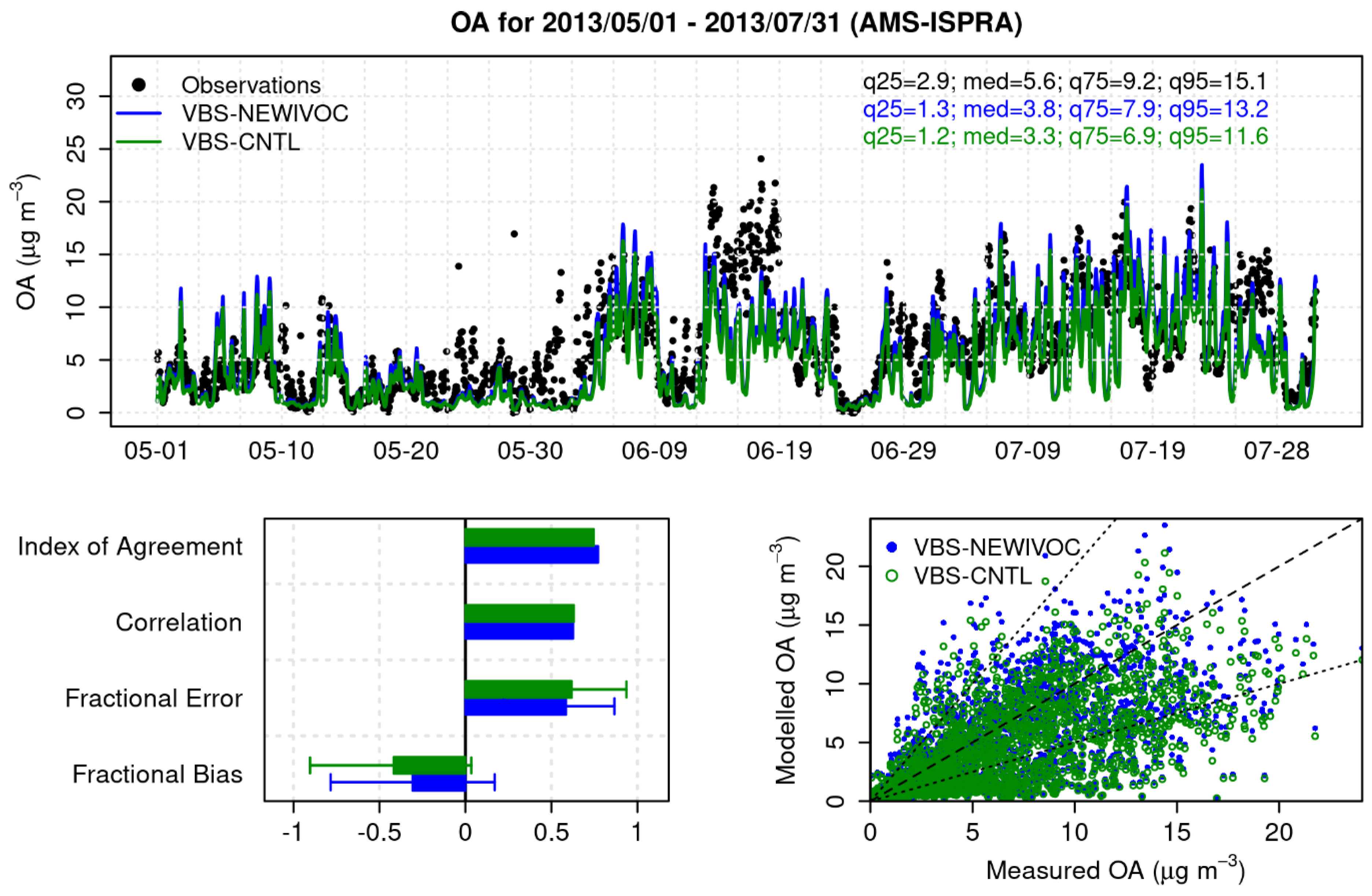
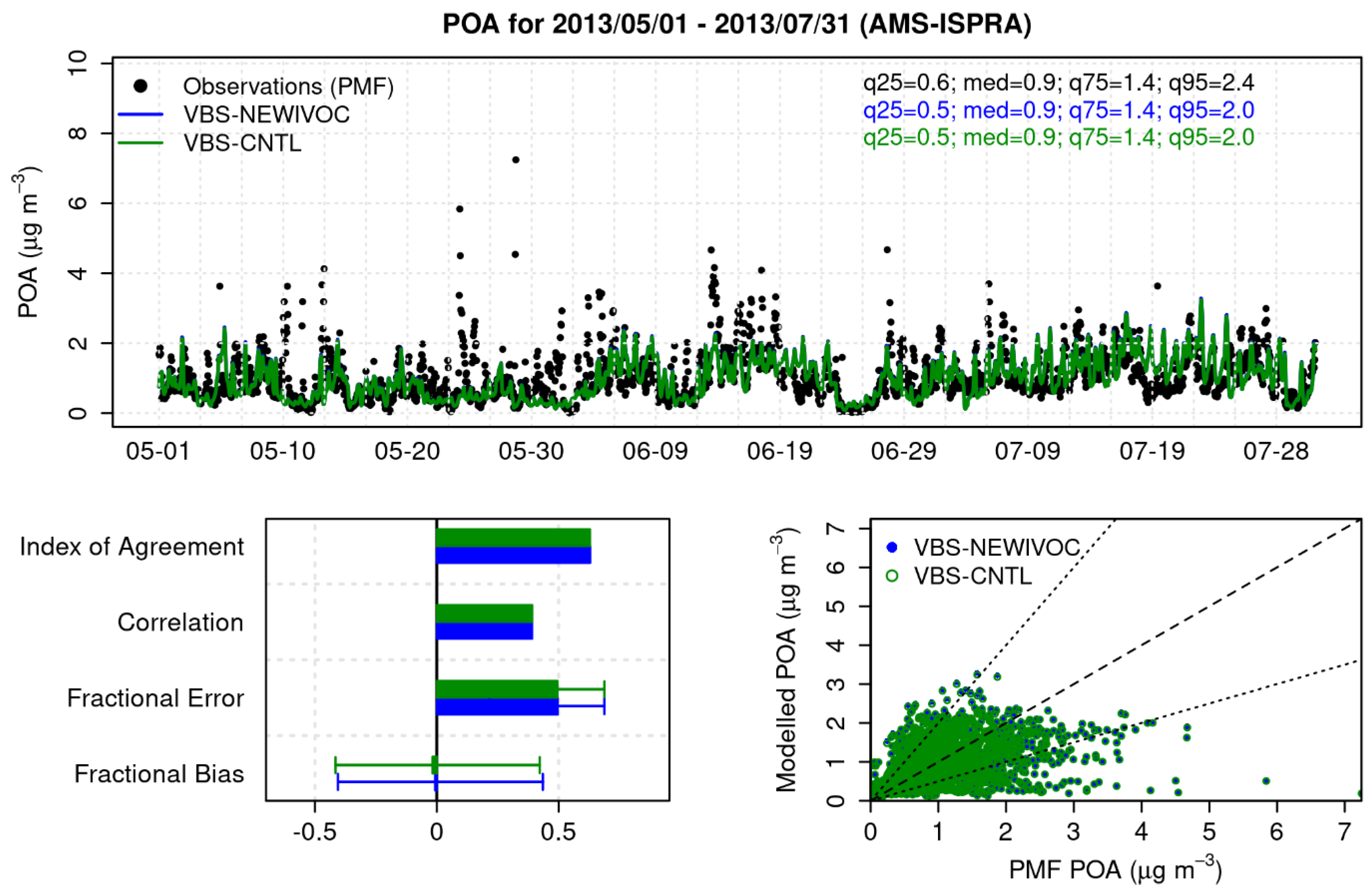
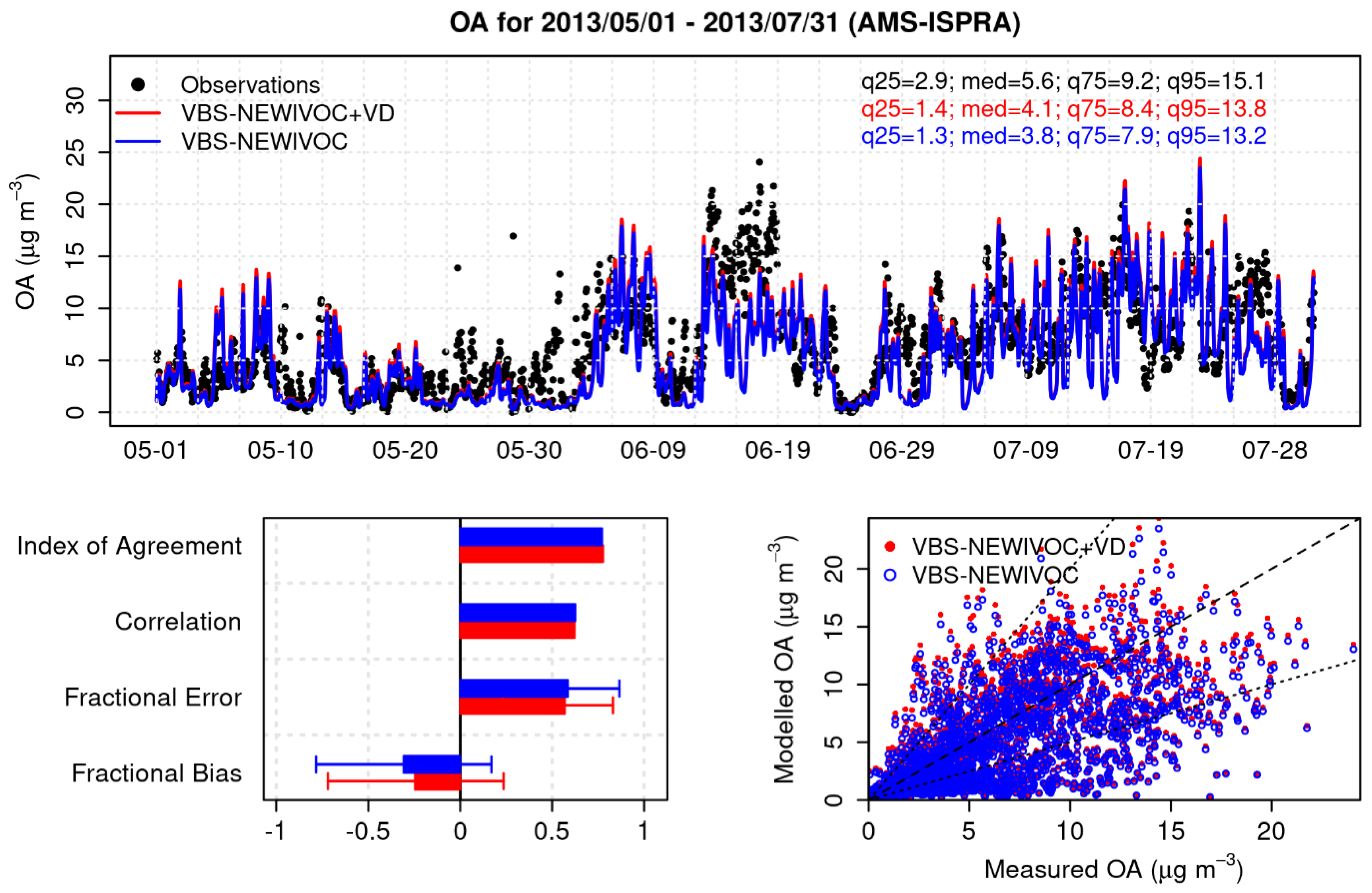
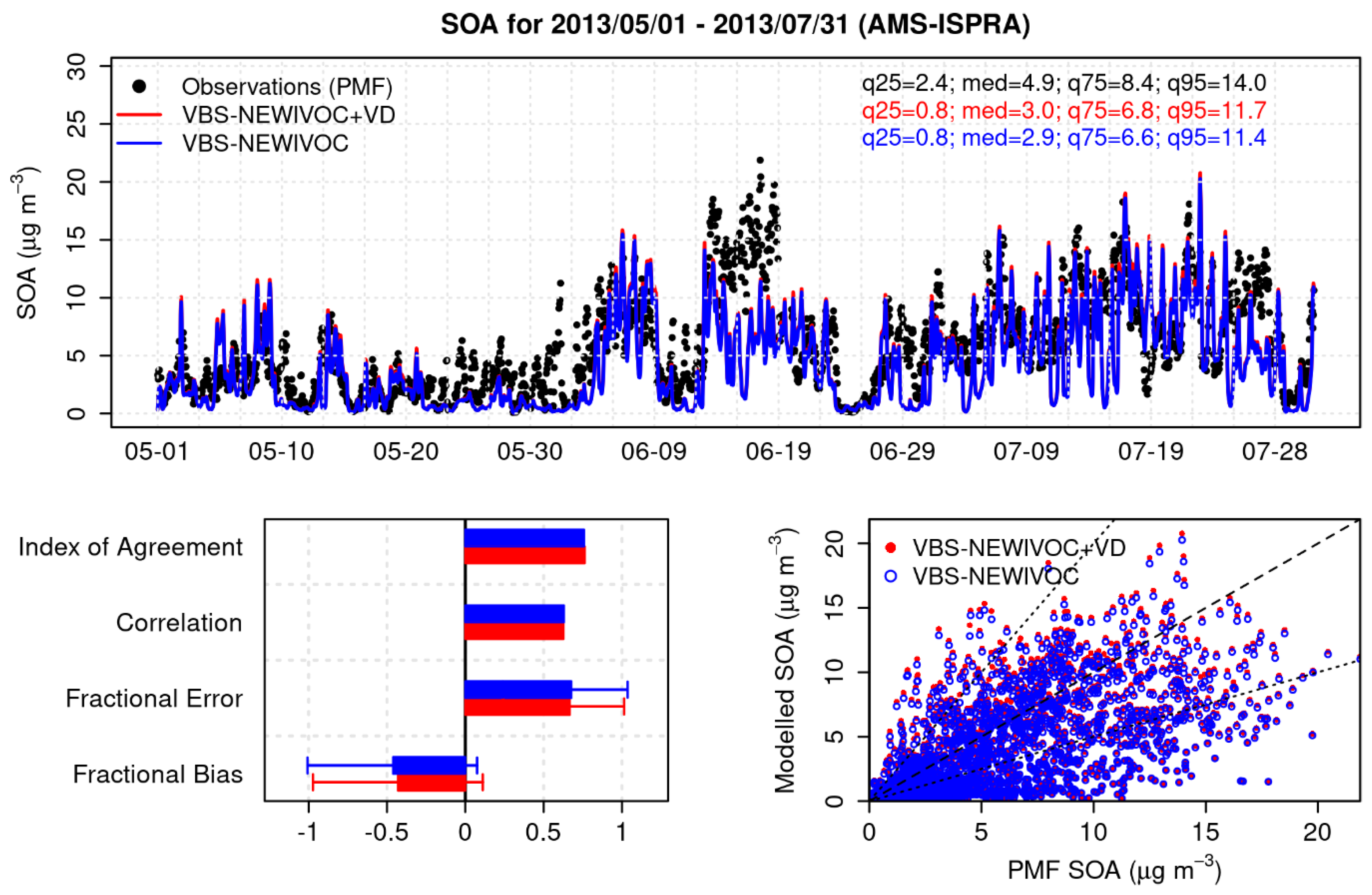
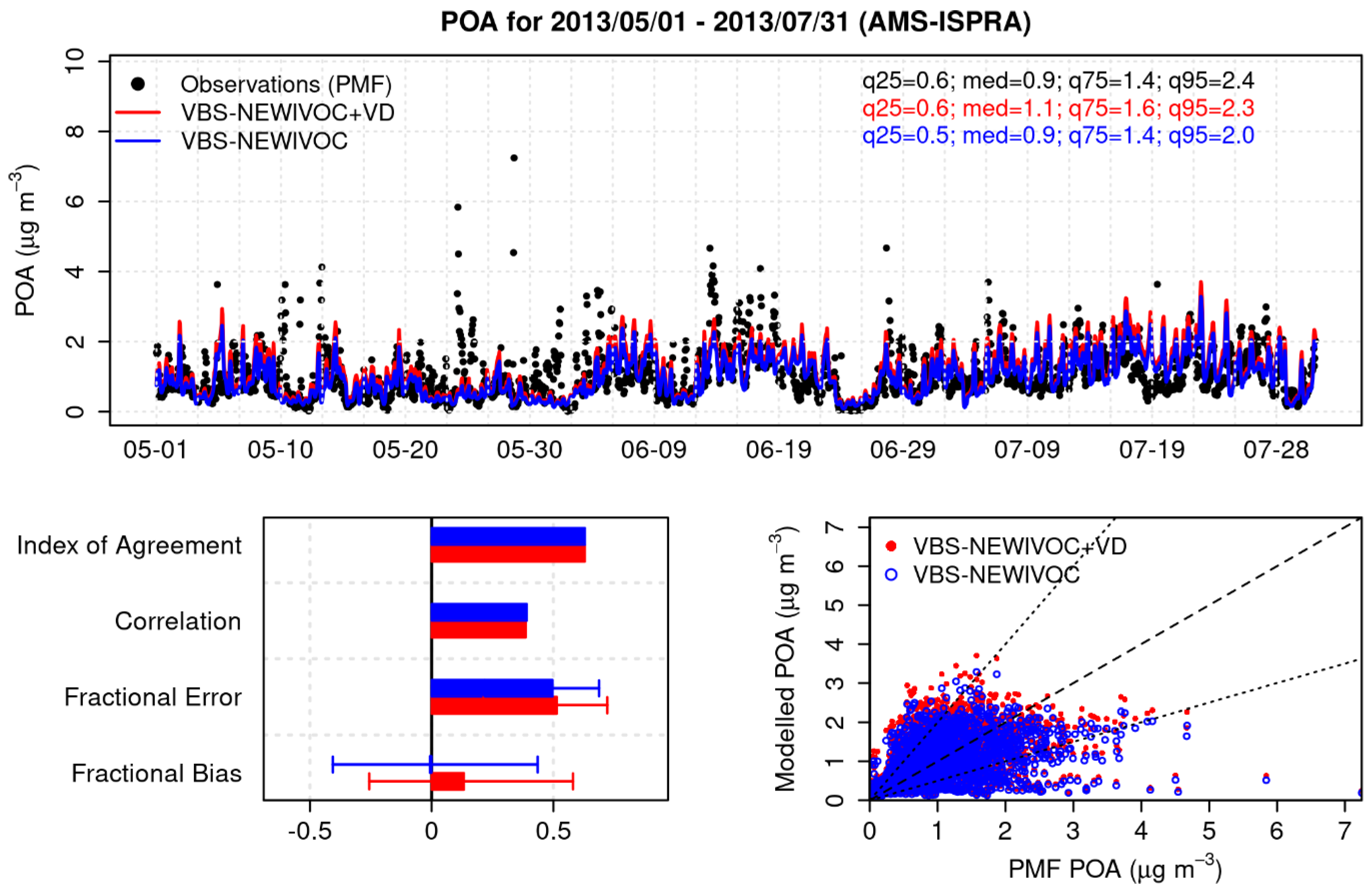
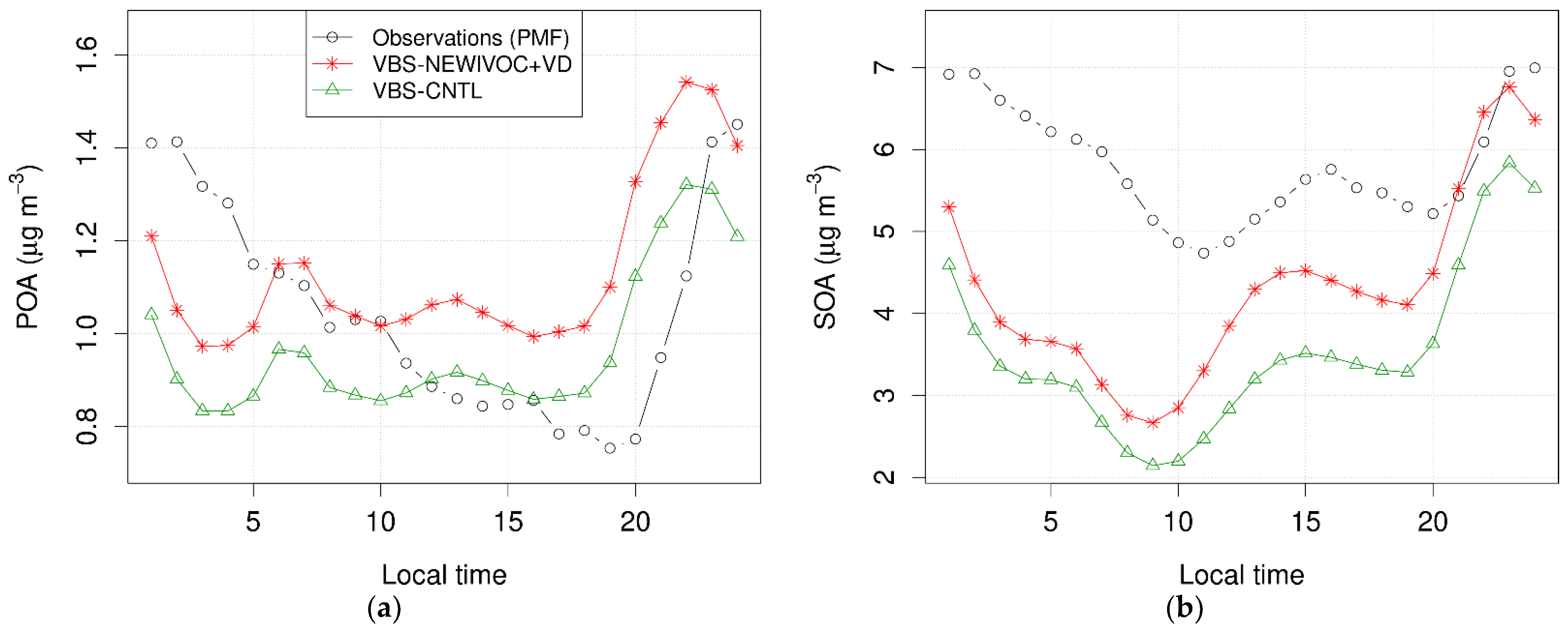
3.2.1. Ispra Site

At this site, OA data are available for the whole quarter, with hourly concentration levels usually below 10 µg m⁻³ except for a mid-June week, when OA was constantly in the 10–20 µg m⁻³ range, and for some isolated peak events in late July. Values of the performance indicators computed for OA, POA, SOA, as well as for hydrocarbon-like OA (HOA) and biomass burning OA (BBOA) in VBS simulations, are summarized for the four simulations in Table S1. Base-case SOAP and VBS simulations give similar results with a fairly good agreement with observations (IOA = 0.75), though with a common underestimation tendency (MB = −1.6 µg m⁻³ for SOAP-CNTL and −2.0 µg m⁻³ for VBS-CNTL) but both missing the high concentration period in June (Figure S13). Due to the partial transfer of POA to the vapor phase, the VBS scheme estimates slightly lower concentrations of OA, thus worsening the performance of the model, especially in terms of MFB (from −24.7% to −41.8%). The performance of the VBS scheme improves with the revision of IVOC parametrization: IOA increases from 0.75 to 0.77, MFB decreased from −41.8% to −30.8%, and the MB (−1.4 µg m⁻³) becomes even smaller than for SOAP-CNTL (Figure 1). Still, the model is not able to reproduce some of the high-concentration events observed in June and July that are mainly responsible for the negative bias of the simulation. Such a better performance was the consequence of a more accurate reproduction of both the primary and, most of all, of the secondary fraction of OA, which accounts for more than 80% of OA mass. For SOA (Figure 2), the improvement is shown by the increased IOA (from 0.72 for VBS-CNTL to 0.76) and the reduction in MFB (from −60.0% to −46.1%). For POA (Figure 3), improvements come with a slightly lower MFB (from −1.8% to −0.7%), due to small changes in the reproduction of its main fractions, HOA (hydrocarbon-like OA) and BBOA (biomass-burning OA). With respect to VBS-CNTL, the MFB for HOA decreases from −41.8% to −40.6%, with IOA still about 0.62; conversely, MFB for BBOA increases from 44.1% to 45.0%, with no substantial change for IOA (from 0.27 to 0.28). Thus, HOA remains underestimated and BBOA overestimated (Figure S14) and their extremely limited variations did not affect the agreement between the observed and simulated overall concentrations of POA (Figure 3). Concerning BBOA, it is worth noticing that VBS simulations in the June–July period estimate concentration levels similar to those of the previous month of May, on average around 0.5 µg m⁻³, whereas the concentrations obtained from the PMF analysis are constantly zero. In fact, PMF analysis, separately conducted for the months March–May and June–August [29], fails to identify the presence of BBOA in the OA mass of the warmer months, probably due to an actual contribution too small to be quantified by the statistical model. Nevertheless, a wrong time pattern for BBOA emissions in the summer period could also be responsible for the observed mismatch between model results and observations. Thus, the performance indicators for BBOA are computed over the month of May only (Table S2). However, the overestimation of BBOA in June–July does not significantly affect the performance of the model for POA and total OA over the whole quarter because of the small contribution of BBOA to the OA mass in the summer period.

The introduction of the OA volatility revisions in the VBS scheme results in a further improvement in the overall model performance (Figure 4), with an additional reduction in MFB (from −30.8% to −24.6%) and an increase in IOA (from 0.77 to 0.78), once again driven by the better reproduction of SOA in spite of a worse reproduction of POA. For SOA (Figure 5), MFB decreases to −43.0% (from −46.1%) and IOA increases to 0.78 (from 0.77); conversely, for POA (Figure 6), MFB increases to 13.3% (from −0.7%) with no change for IOA (0.63). The positive MFB for POA is determined by the additional overestimation of BBOA fraction (MFB = 61.6%) that offsets the better reproduction of HOA (Figure S15), characterized by reduced underestimation (MFB from −40.6% to −31.5%) and increased agreement (IOA from 0.62 to 0.64). Nevertheless, in spite of the better general performance, the model is still not able to reproduce the high concentration event in mid-June, when SOA concentrations remained largely underestimated. During those days, peculiar meteorological conditions, driven by rather low wind speed and very high relative humidity values, resulted in enhanced secondary formation processes that are generally captured and even overestimated by CAMx, as also suggested by the high concentrations of secondary sulfate. The only exception is OA, mainly driven by SOA underestimation, suggesting that some OM formation processes are not properly reproduced yet.

The analysis of the daily time patterns shows different behaviors for SOA and POA reproduction but with the common feature of a strong underestimation of nocturnal concentration levels (Figure 7). On average, the time pattern of SOA is well reproduced but with a 2 h anticipation and clear underestimation (up to about 2.5 µg m⁻³) for almost the whole day that not even both VBS revisions are able to fill. Conversely, for POA the model encounters greater trouble with the daily pattern but reasonably captures the magnitude of the concentration levels likely due to BBOA overestimation balancing HOA underestimation. The difficulty of the model in reproducing the time pattern of POA is mainly caused by the poor reproduction of the time profile of HOA (Figure S16), likely because of the missed decrease in their emission in the central hours of the day (Figure S21) and a possible underestimation of the nighttime accumulation.

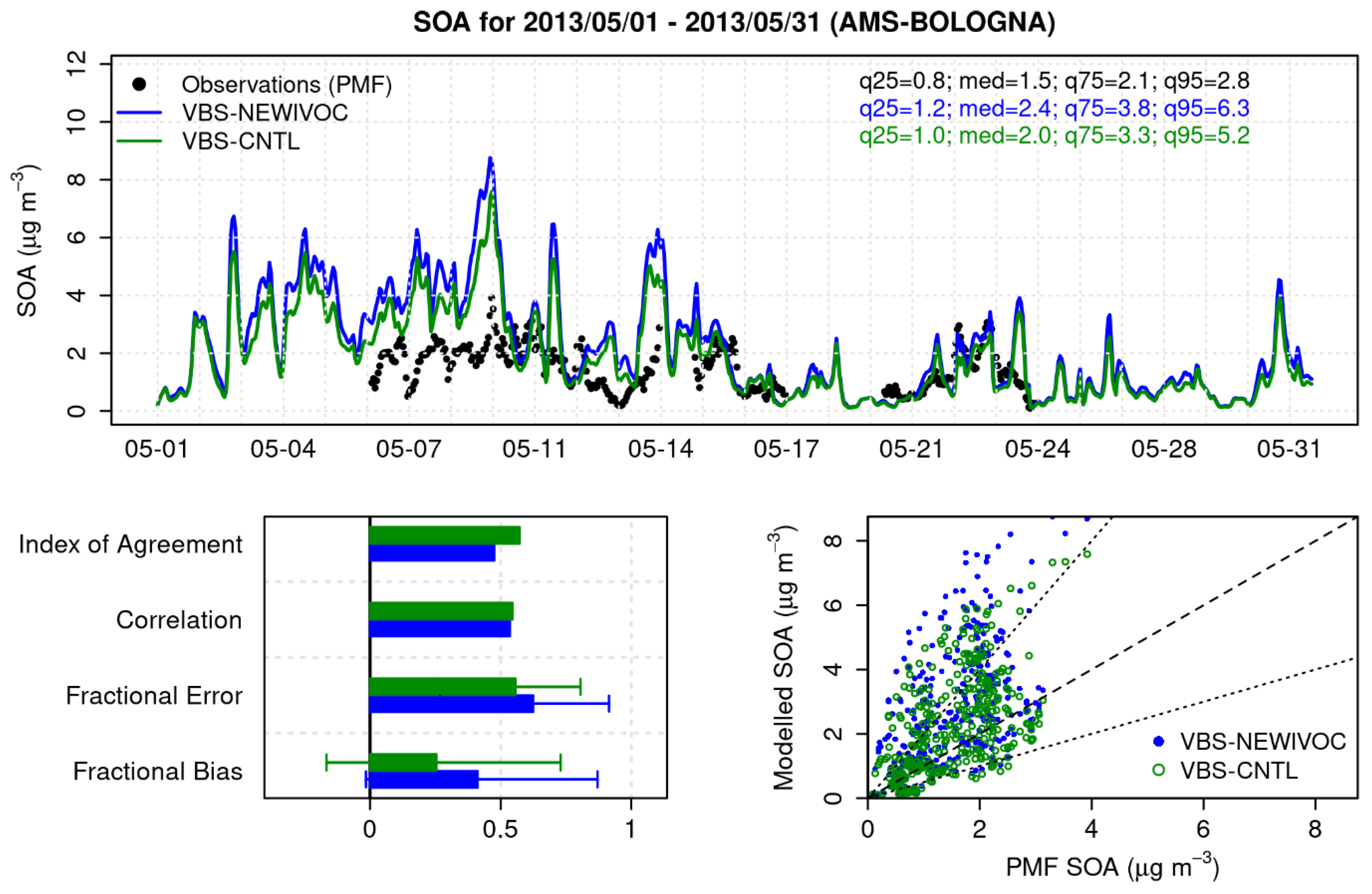
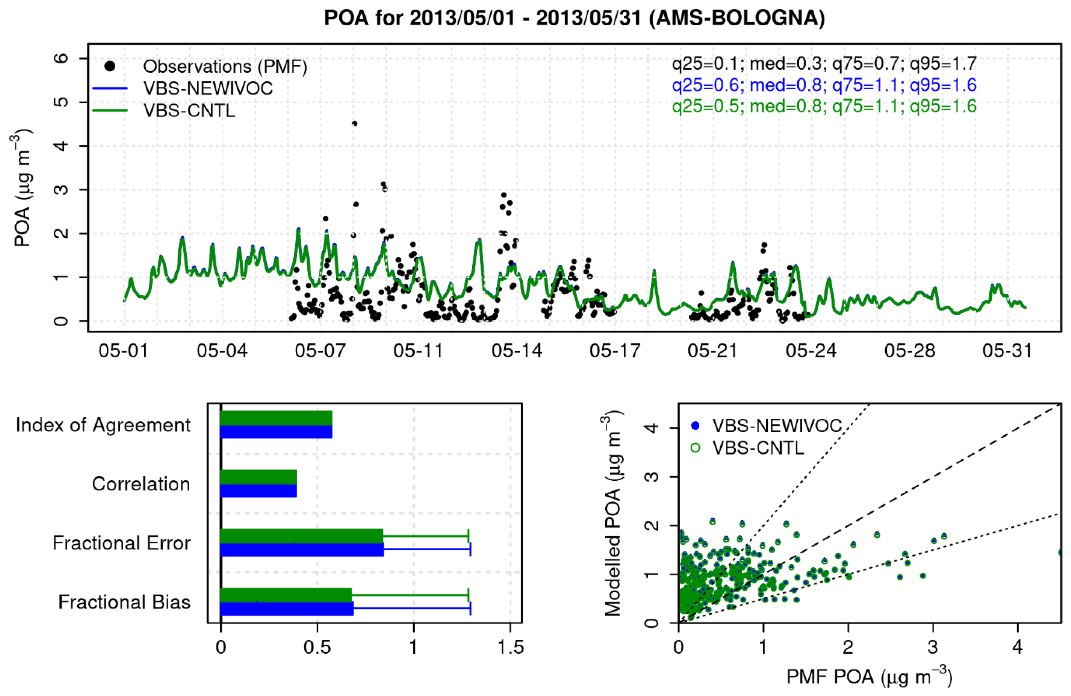
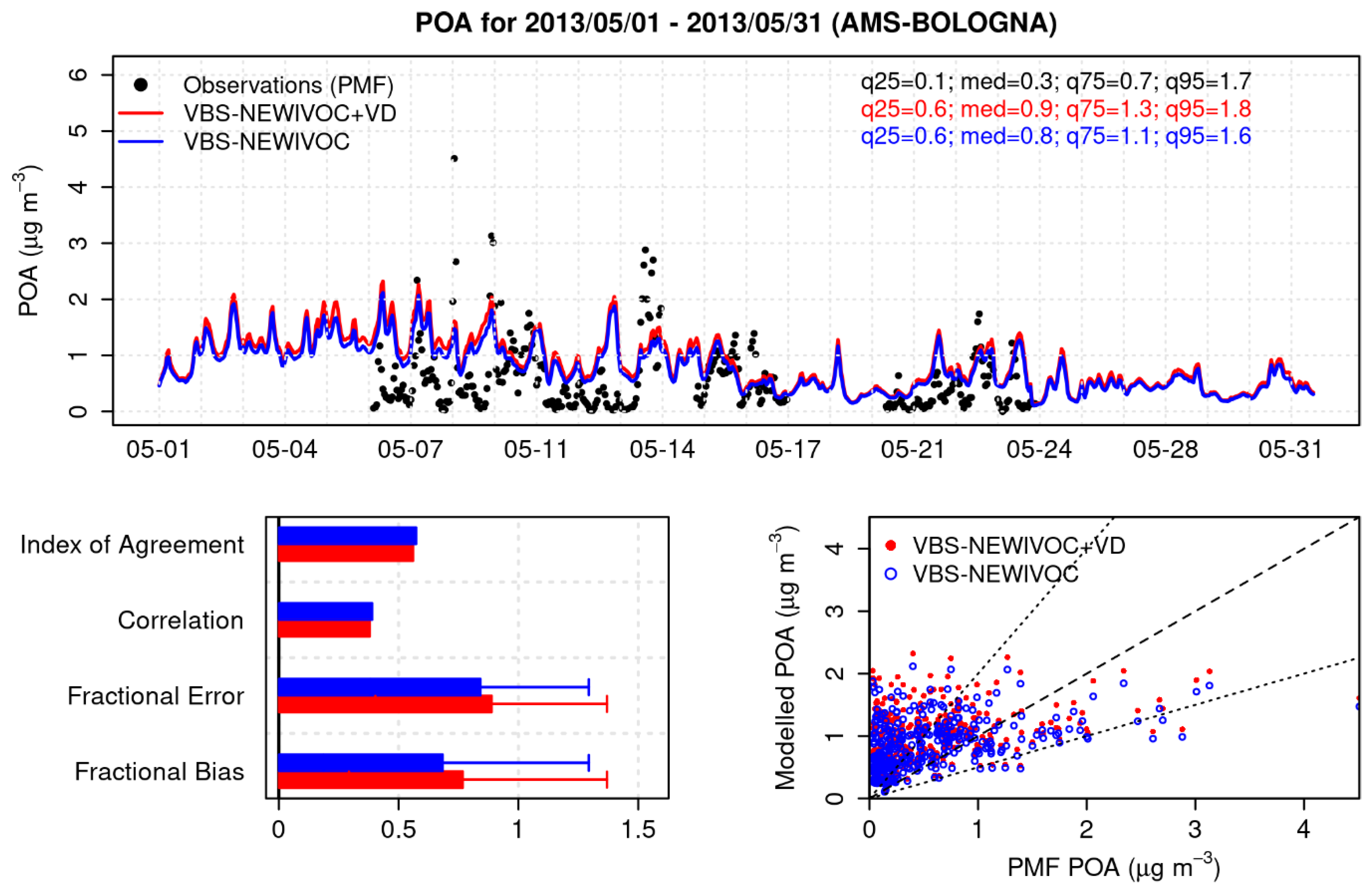
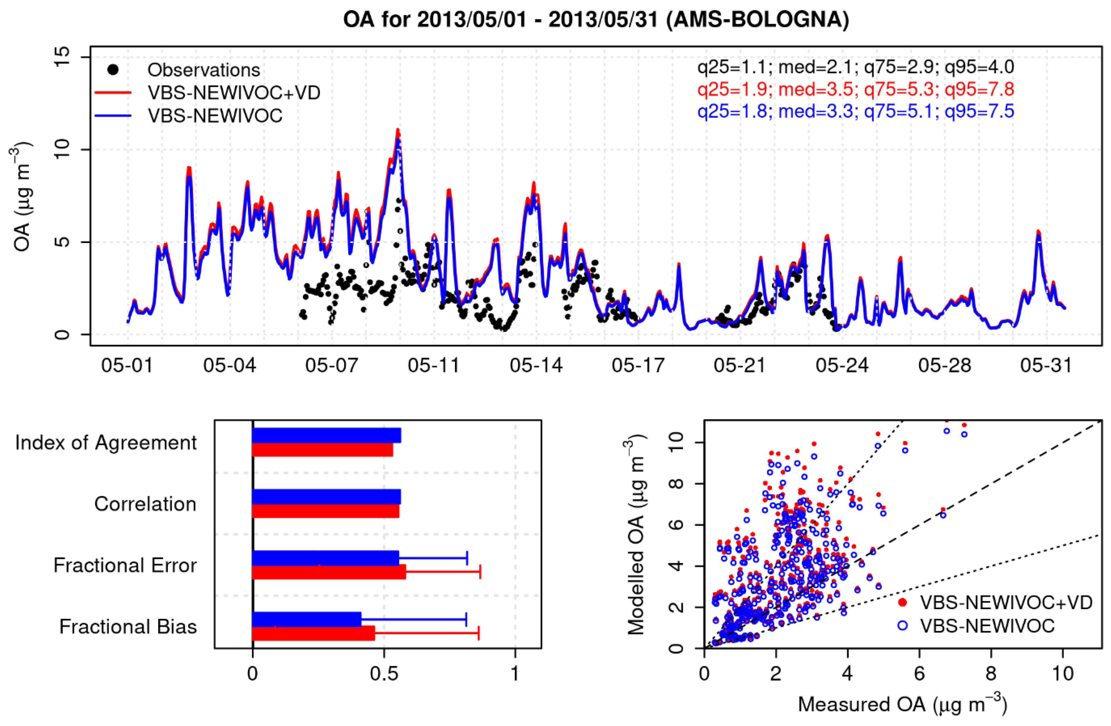
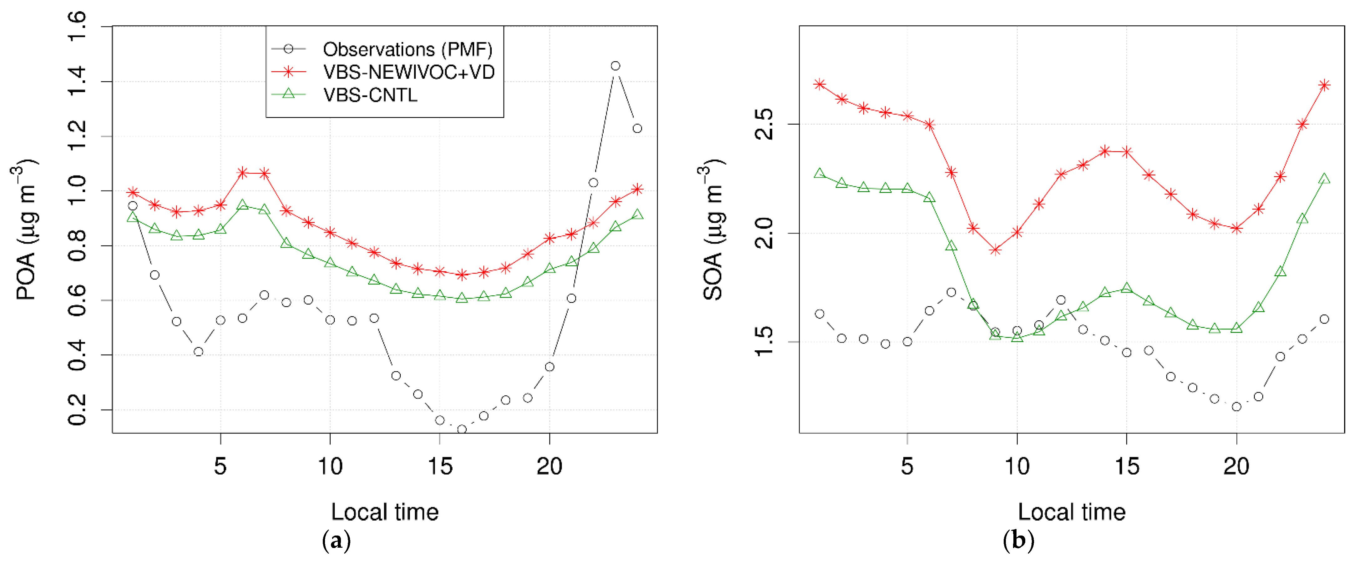
3.2.2. Bologna Site

At this site, OA data are available only for May (6th–24th), with hourly concentration levels usually below 4 µg m⁻³ and an isolated peak event on May 9th (values up to about 8 µg m⁻³). Values of the performance indicators computed for total OA and its components are summarized in comparison with the four simulations in Table S3. SOAP and VBS control simulations (Figure S17) give similar results but with lower agreement with observations and a larger overestimation tendency for SOAP (MB = 1.25 µg m⁻³, IOA=0.62, Table S3) than for the VBS scheme (MB = 0.98 µg m⁻³ IOA=0.65). In fact, the VBS scheme is more accurate on POA reproduction (MFB = 67.4% vs. 92.0% of SOAP), while behaving similarly to SOAP on SOA (MFB = 25.5% vs. 29.2% of SOAP).

The revised IVOC parametrization worsens the performance of the VBS scheme for OA (Figure 8), with a larger bias and error and a lower agreement (IOA = 0.65) because of the increased SOA levels (Figure 9). MB (1.23 µg m⁻³) and MFB (41.2%) for SOA are almost double than in the base case (0.76 µg m⁻³ and 25.5%, respectively), whilst POA concentration does not show relevant change (Figure 10) and remains slightly overestimated, overall (MFB = 68.5%) and in both its fractions (MFB = 78.5% for HOA and 62.7% for BBOA, Figure S18). The further revisions on OA volatility increase the overestimation of both SOA (Figure 11) and POA (Figure 12), and consequently of the overall OA concentration levels (Figure 13). For OA, MB rose up to 1.67 µg m⁻³ (from 0.98 µg m⁻³ in VBS base case) and MFB to 46.3% (from 29.3%), so that IOA is as low as 0.53 (from 0.62). The revisions mostly affect the BBOA fraction (Figure S19), whose MFB increase by 15% (up to 77.6%), whereas HOA (Figure S19) and SOA suffer only a 3% increase in their MFBs. Thus, the clear overestimation of OA concentrations at the beginning of the monitoring period, already present in the base case and affecting all OA fractions, increases even more with the introduction of VBS revisions and lowers the performance of the model.

The analysis of the daily patterns (Figure 14) clearly highlights the overestimation of both POA and SOA, which already affects the base case VBS simulation and is further increased by the IVOC and volatility revisions but shows that the shape of the concentration profiles was satisfactorily reproduced. However, the model simulations depict POA profiles that miss the fairly constant concentration levels observed in the morning, their sharp decrease in the afternoon, and the magnitude of the evening peak, actually driven by a few events (3 days with POA in the 2–3 µg/m³ range at 11 PM). As for the site of Ispra, the model difficulties with the time pattern are mainly caused by the wrong reproduction of HOA time profile (Figure S20), which is almost constant in the model results. Such a discrepancy is probably related to an underestimation of atmospheric dispersion, as shown by the underestimation of the wind speed in Bologna, particularly during afternoon hours (Figure S5) and also partially enhanced by the hourly emission profile (Figure S21) characterized by an almost flat profile during the central hours of the day. SOA levels are systematically overestimated throughout the whole day, with the only exception of morning hours in VBS-CNTL simulation when they exactly match the observations. Despite the overestimation, the time pattern of SOA is better reproduced, albeit with some difficulty in the early afternoon hours, due to the delay in the concentration decrease.

4. Discussion

In general, enhancing the VBS scheme with revisions on the IVOCs parameterizations and on the volatility classes does not show particularly clear effects on the results of the simulations for the spring–summer period. The revisions on IVOC emissions mainly lead to the increase in SOA concentrations, while those on OM volatility lead to the increase in POA concentrations. These effects are clearly highlighted in Figure 15, which shows the spatial distribution of the additional response of the VBS scheme, first to IVOC emission revisions (middle panels), then to OM volatility (right panels), in terms of contributions to the average concentrations of POA and SOA over the Po Valley for the summer quarter from May to July 2013. In particular, the variations of POA are localized around the main emission areas. Instead, those of SOA, precisely due to its secondary nature, are more uniformly distributed in the basin. However, larger variations still occur in correspondence with the more urbanized areas, where the emissions of precursors are greater.

Simulation results for the spring–summer period indicate that the new parametrizations lead to variations in estimated OA concentrations less relevant than those found for the winter case [13] and mostly related to SOA. With respect to the VBS base case, at the two reference sites the increase in POA and SOA monthly concentrations for May 2013 is in the 13.1–22.4% range (i.e., 0.10–0.15 µg m⁻³) and in the 16.2–26.7% range (i.e., 0.44–0.47 µg m⁻³), respectively; corresponding figures for March 2013 are in the 10.6–31.4% range (i.e., 0.90–1.21 µg m⁻³) for POA and in the 136.8–155.4% range (i.e., 2.02–2.60 µg m⁻³) for SOA. The smaller effect observed for the warm season estimates is reasonably due to the combination of different reasons:

• The changes in IVOC emissions only concern anthropogenic sources (road traffic and biomass combustion), but the effects of those relating to biomass combustion are counterbalanced by the significant reduction in the activity of this source in the warm season;
• In the warm season, SOA of biogenic origin contribute much more significantly to the overall mass of SOA, thus masking the effect of the increased anthropogenic emissions;
• Warm season conditions, namely, ambient temperature, favor the partitioning of organic compounds in the vapor phase rather than in the particulate one, contributing to further limiting the effect of the increased IVOC emissions on aerosol production.

Even though limited to a few tenths of µg m⁻³, the increase in POA and SOA concentrations has a different impact on total OA reproduction at the reference sites in the warm season, compared with the cold season, as shown by the pie charts (Figure 16 and Figure 17) in March and May of 2013. In the cold season, VBS-CNTL results largely underestimate OA concentration at both sites: at Ispra and Bologna missing OA mass is about 10.1 µg m⁻³ (67% of the observed 14.9 µg m⁻³) and 4.1 µg m⁻³ (50% of the observed 8.0 µg m⁻³), respectively. Thus, at both sites the larger amount of POA and SOA estimated by the enhanced VBS with emission revisions (VBS-NEWIVOC+VD) is beneficial for a better reproduction of OA concentrations, though still not complete: at Ispra the missing OA mass is reduced to 6.25 µg m⁻³ (still 41.8% of the observed OA) and at Bologna to 1.15 µg m⁻³ (only 14.3% of the observed OA). Conversely, in the warm season VBS-CNTL underestimates OA concentration at Ispra but slightly exceeds the observations at Bologna. Thus, the additional OA mass estimated by the enhanced VBS scheme (about 0.6 µg m⁻³ at both sites) improves its performance at the former site and worsens it at the latter, as shown by the values of the performance indicators in Tables S2 and S3.

Further investigation is needed to identify the origin of the remaining missing mass, although a few possible mechanisms can be hypothesized. The relevant sensitivity of CAMx results in changes in IVOC emissions and volatility distributions which suggest that formation processes related to anthropogenic sources play a relevant role, particularly during the cold season, that is probably not completely captured by CAMx. It is worth noting that CAMx considers only gas phase formation, while neglecting aqueous phase processes that can also contribute to OM formation. Additional uncertainties could be related to biogenic SOA (BSOA) production related to biogenic VOC emissions and the fine fraction of pollen emissions, which is not considered by the model but possibly relevant during the summer season.

The revisions reduce the missing OA mass from 1.24 µg m⁻³ to 0.65 µg m⁻³ (from 46.3% to 24.2%) at Ispra, while they increase the excess mass from 0.52 µg m⁻³ to 1.10 µg m⁻³ (from 25.1% to 53.1%) at the Bologna site. Such an opposite effect is influenced by the different OA levels observed at the two sites, with OA concentrations at Ispra about 50% higher than at Bologna (3.56 µg m⁻³ vs. 2.07 µg m⁻³). Therefore, the obtained results confirm that IVOC emissions and volatility revisions also give rise to an overall increment of OA concentration in the summer season, additionally contributing to a better allocation between primary and secondary fraction. However, such a result does not always give rise to a better reproduction of OA because the overall performance of the modeling system is related to several factors. CAMx shows a general overestimation of PM_2.5 and PM₁₀ observations, especially during May and the first half of June (Figure S8); therefore, it is reasonable that in Bologna OM concentrations are also overestimated. In this case, the modeling improvement due to the introduction of IVOC emissions and the revision of volatility does not result in a corresponding improvement in model performance. This is confirmed by the results obtained for the rural site of San Pietro Capofiume, located about 30 km from Bologna, characterized by even lower OA concentrations (1.4 µg m⁻³ in May 2013). Similarly to the Bologna site, at San Pietro Capofiume the overprediction of OA concentration already obtained with the VBS-CNTL simulation (MB = 0.65 µg m⁻³) is further increased (MB = 0.99 µg m⁻³) by the introduction of all the revisions (Table S4, Figure S22).

At the Ispra site, the domain-wide overestimation related to wind speed underestimation and partial relative humidity overestimation seems to be partially smoothed by local effects. Indeed, Ispra is a rural site close to the hilly area of the Prealps and, as a consequence, neither the spatial emission distribution (particularly from road transport) nor the local circulation features are well captured at 5 km resolution. These local scale inconsistencies lead to an excessive dilution of pollution and therefore to the underestimation of the observed values. Such local effects in Ispra seem to prevail compared with the previously mentioned domain-wide effect that promotes pollutant accumulation. The resulting underestimation of OM concentration in Ispra is partially solved by the modeling improvements.

Figure 16 and Figure 17 also show that the divergence between observed and modeled OA concentrations, both as under- and overestimates, is mainly due to SOA reproduction; conversely, the estimated POA (i.e., HOA + BBOA) better matches the observations, except for Ispra in the cold season, when both its components are also underestimated by the VBS-NEWIVOC+VD simulation. Concerning the excess SOA predicted at Bologna in May, it is worth noticing that the monthly average is strongly affected by the clear overestimation at the beginning of the monitoring period (Figure 9), when model results are 2–3 times higher than the observations. As already mentioned, this is probably due to issues with the reproduction of the meteorological conditions over the eastern part of the Po Valley, as clearly pointed out by the corresponding overestimation of the inorganic PM compounds. As already discussed, Figure 16 and Figure 17 show that the revisions lead to small variations of the estimated total POA concentrations in the warm season and mostly affect SOA levels, both in terms of anthropogenic SOA (ASOA, i.e., SOA from precursors emitted by human activities, namely, road traffic) and biogenic SOA (BSOA), which includes SOA due to precursors from natural emission and biomass burning activity.

5. Conclusions

Results of the sensitivity analysis of the CAMx model in reconstructing the organic aerosol (OA) concentrations in the Po Valley with different chemical schemes are presented. Model simulations refer to the warm season quarter May–July 2013 and include control cases with the default SOAP and VBS scheme, and those with the VBS scheme with revisions in the estimates of emissions of intermediate volatility organic compounds (IVOC) and with new distributions of volatility for primary organic matter. Model results are compared with sets of OA composition obtained from the PMF analysis of experimental data from measurement campaigns carried out at two sites in the area.

Simulation results show that, in general, the VBS scheme leads to slight underestimation of the OA concentration than the SOAP scheme because of the partial transfer to the vapor phase of the primary organic aerosol (POA). This improves the performance of the model over the rural and suburban areas in the eastern part of the Po Valley, characterized by low OA levels, overestimated by SOAP; conversely, it worsens the performance in the northwestern part, where OA levels, almost twice as high, are underestimated by SOAP. The enhancement of the VBS scheme with revisions of IVOC emissions and of the volatility characteristics of primary emissions lead to an increase in the estimated concentrations of both the primary (POA) and secondary components (SOA) of the organic aerosol because of the overall increase in the organic component of the anthropogenic emissions (road traffic and biomass combustion), likely still underestimated in the current emission inventories.

Although limited to a few tenths of µg m⁻³, the revisions on IVOC emissions lead to an increase in SOA concentrations, while those on volatility mainly lead to an increase in POA concentrations. These additional contributions to the estimated OA mass determine improvements or worsening of the model performance depending on the concentration levels locally observed. However, with reference to the total OA, the introduction of these revisions does not produce clear effects in the results of the summer simulations, as opposed to the winter case discussed in previous studies. In fact, the changes introduced concern anthropogenic emissions that in summer have less importance than in the winter period: the contribution of biomass combustion source is greatly reduced and, on the contrary, emissions of biogenic origin increase. In addition, the revisions act on the particulate component which decreases in the warm season because of the greater volatility of organic compounds as a result of the higher atmospheric temperature.

The new IVOC parameterizations used in this work seem to provide coherent results with the previous application focused on the winter season, but further experimental studies would be needed (especially over a European domain) to better evaluate the emissions of organic compounds with intermediate volatility and thus use less general and more site-specific parameterization methods for the different study areas. Furthermore, given the systematic overestimation of the OA component associated with biomass combustion emissions in the summer period, it would be necessary to check the accuracy of the inventory data for this source and to revise the seasonal regime of sources’ activity. Finally, it is evident that a correct meteorological simulation is essential to accurately reproduce the atmospheric processes that impact on the reproduction of the OA concentration. In fact, values showing significant divergences between observed and modeled OA concentrations are probably due to a difficult and inaccurate reproduction of the local meteorological conditions.

In conclusion, the VBS scheme with emission revisions looks promising for a better reproduction of organic aerosol. However, further modeling studies and, most of all, experimental campaigns for speciated organic aerosol are required in order to strengthen our results and overcome the limitations of this work, which is essentially related to the short time period analyzed and to the limited number of reference sites considered.

References

- Targa, J.; Ripoll, A.; Banyuls, L.; González, A.; Soares, J. Status Report of Air Quality in Europe for Year 2020, Using Validated Data (Eionet Report—ETC/HE 2022/2). 2022. Available online: https://www.eionet.europa.eu/etcs/etc-he/products/etc-he-products/etc-he-reports/etc-he-report-2022-2-status-report-of-air-quality-in-europe-for-year-2020-using-validated-data (accessed on 6 November 2022).
- Nault, B.A.; Jo, D.S.; McDonald, B.C.; Campuzano-Jost, P.; Day, D.A.; Hu, W.; Schroder, J.C.; Allan, J.; Blake, D.R.; Canagaratna, M.R.; et al. Secondary organic aerosols from anthropogenic volatile organic compounds contribute substantially to air pollution mortality. Atmos. Chem. Phys. 2021, 21, 11201–11224. [Google Scholar] [CrossRef]
- Chang, X.; Zhao, B.; Zheng, H.; Wang, S.; Cai, S.; Guo, F.; Gui, P.; Huang, G.; Wu, D.; Han, L.; et al. Full-volatility emission framework corrects missing and underestimated secondary organic aerosol sources. One Earth 2022, 5, 403–412. [Google Scholar] [CrossRef]
- Patoulias, D.; Kallitsis, E.; Posner, L.; Pandis, S.N. Modeling Biomass Burning Organic Aerosol Atmospheric Evolution and Chemical Aging. Atmosphere 2021, 12, 1638. [Google Scholar] [CrossRef]
- Bergström, R.; van der Gon, H.A.C.D.; Prévôt, A.S.H.; Yttri, K.E.; Simpson, D. Modelling of organic aerosols over Europe (2002–2007) using a volatility basis set (VBS) framework: Application of different assumptions regarding the formation of secondary organic aerosol. Atmos. Chem. Phys. 2012, 12, 8499–8527. [Google Scholar] [CrossRef]
- Woody, M.C.; Baker, K.R.; Hayes, P.L.; Jimenez, J.L.; Koo, B.; Pye, H.O.T. Understanding sources of organic aerosol during CalNex-2010 using the CMAQ-VBS. Atmos. Chem. Phys. 2016, 16, 4081–4100. [Google Scholar] [CrossRef]
- Hodzic, A.; Jimenez, J.L.; Madronich, S.; Aiken, A.C.; Bessagnet, B.; Curci, G.; Fast, J.; Lamarque, J.-F.; Onasch, T.B.; Roux, G.; et al. Modeling organic aerosols during MILAGRO: Importance of biogenic secondary organic aerosols. Atmos. Chem. Phys. 2009, 9, 6949–6981. [Google Scholar] [CrossRef]
- Donahue, N.M.; Epstein, S.A.; Pandis, S.N.; Robinson, A.L. A two-dimensional volatility basis set—Part 1: Organic-aerosol mixing thermodynamics. Atmos. Chem. Phys. 2011, 11, 3303–3318. [Google Scholar] [CrossRef]
- Donahue, N.M.; Kroll, J.H.; Pandis, S.N.; Robinson, A.L. A two-dimensional volatility basis set—Part 2: Diagnostics of organic-aerosol evolution. Atmos. Chem. Phys. 2012, 12, 615–634. [Google Scholar] [CrossRef]
- Huang, L.; Wang, Q.; Wang, Y.; Emery, C.; Zhu, A.; Zhu, Y.; Yin, S.; Yarwood, G.; Zhang, K.; Li, L. Simulation of secondary organic aerosol over the Yangtze River Delta region: The impacts from the emissions of intermediate volatility organic compounds and the SOA modeling framework. Atmos. Environ. 2020, 246, 118079. [Google Scholar] [CrossRef]
- Ots, R.; Young, D.E.; Vieno, M.; Xu, L.; Dunmore, R.E.; Allan, J.D.; Coe, H.; Williams, L.R.; Herndon, S.C.; Ng, N.L.; et al. Simulating secondary organic aerosol from missing diesel-related intermediate-volatility organic compound emissions during the Clean Air for London (ClearfLo) campaign. Atmos. Chem. Phys. 2016, 16, 6453–6473. [Google Scholar] [CrossRef]
- Dunmore, R.E.; Hopkins, J.R.; Lidster, R.T.; Lee, J.D.; Evans, M.J.; Rickard, A.R.; Lewis, A.C.; Hamilton, J.F. Diesel-related hydrocarbons can dominate gas phase reactive carbon in megacities. Atmos. Chem. Phys. 2015, 15, 9983–9996. [Google Scholar] [CrossRef]
- Giani, P.; Balzarini, A.; Pirovano, G.; Gilardoni, S.; Paglione, M.; Colombi, C.; Gianelle, V.L.; Belis, C.A.; Poluzzi, V.; Lonati, G. Influence of semi- and intermediate-volatile organic compounds (S/IVOC) parameterizations, volatility distributions and aging schemes on organic aerosol modelling in winter conditions. Atmos. Environ. 2019, 213, 11–24. [Google Scholar] [CrossRef]
- Ciarelli, G.; El Haddad, I.; Bruns, E.; Aksoyoglu, S.; Möhler, O.; Baltensperger, U.; Prévôt, A.S.H. Constraining a hybrid volatility basis-set model for aging of wood-burning emissions using smog chamber experiments: A box-model study based on the VBS scheme of the CAMx model (v5.40). Geosci. Model Dev. 2017, 10, 2303–2320. [Google Scholar] [CrossRef]
- Zhao, Y.; Nguyen, N.T.; Presto, A.A.; Hennigan, C.J.; May, A.A.; Robinson, A.L. Intermediate Volatility Organic Compound Emissions from On-Road Diesel Vehicles: Chemical Composition, Emission Factors, and Estimated Secondary Organic Aerosol Production. Environ. Sci. Technol. 2015, 49, 11516–11526. [Google Scholar] [CrossRef] [PubMed]
- Zhao, Y.; Nguyen, N.T.; Presto, A.A.; Hennigan, C.J.; May, A.A.; Robinson, A.L. Intermediate volatility organic compound emissions from on-road gasoline vehicles: Chemical composition, emission factors, and estimated secondary organic aerosol production. Environ. Sci. Technol. 2016, 50, 4554–4563. [Google Scholar] [CrossRef] [PubMed]
- Denier van der Gon, H.A.C.; Bergström, R.; Fountoukis, C.; Johansson, C.; Pandis, S.N.; Simpson, D.; Visschedijk, A.J.H. Particulate emissions from residential wood combustion in Europe—Revised estimates and an evaluation. Atmos. Chem. Phys. 2015, 15, 6503–6519. [Google Scholar] [CrossRef]
- ENVIRON. CAMx (Comprehensive Air Quality Model with Extensions) User’s Guide, Version 6.40; ENVIRON International Corporation: Novato, CA, USA, 2016. [Google Scholar]
- Meroni, A.; Pirovano, G.; Gilardoni, S.; Lonati, G.; Colombi, C.; Gianelle, V.; Paglione, M.; Poluzzi, V.; Riva, G.; Toppetti, A. Investigating the role of chemical and physical processes on organic aerosol modelling with CAMx in the Po Valley during a winter episode. Atmos. Environ. 2017, 171, 126–142. [Google Scholar] [CrossRef]
- Skamarock, W.C.; Klemp, J.B.; Dudhia, J.; Gill, D.O.; Barker, D.M.; Duda, M.G.; Huang, X.-Y.; Wang, W.; Powers, J.G. A Description of the Advanced Research WRF; Version 3; NCAR Technical Note -475+STR; University Corporation for Atmospheric Research: Boulder, CO, USA, 2008. [Google Scholar] [CrossRef]
- UNC—University of North Carolina, Institute for the Environment. SMOKE v3.5 User’s Manual. Chapel Hill. 2013. Available online: https://www.cmascenter.org/smoke/ (accessed on 6 November 2022).
- ISPRA Italian National Inventory Data. Available online: http://emissioni.sina.isprambiente.it/inventario-nazionale/ (accessed on 6 November 2022).
- INEMAR—ARPA Lombardia. Emission Inventory: 2012 Emission in Region Lombardy—Public Review. ARPA Lombardia Settore Aria. 2015. Available online: http://www.inemar.eu/ (accessed on 6 November 2022).
- Guenther, A.; Karl, T.; Harley, P.; Wiedinmyer, C.; Palmer, P.I.; Geron, C. Estimates of global terrestrial isoprene emissions using MEGAN (Model of Emissions of Gases and Aerosols from Nature). Atmos. Chem. Phys. 2006, 6, 3181–3210. [Google Scholar] [CrossRef]
- Gong, S.L. A parameterization of sea-salt aerosol source function for sub- and super-micron particles. Glob. Biogeochem. Cycles 2003, 17, 1097. [Google Scholar] [CrossRef]
- Strader, R.; Lurmann, F.; Pandis, S.N. Evaluation of secondary organic aerosol formation in winter. Atmos. Environ. 1999, 33, 4849–4863. [Google Scholar] [CrossRef]
- Koo, B.; Knipping, E.; Yarwood, G. 1.5-Dimensional volatility basis set approach for modeling organic aerosol in CAMx and CMAQ. Atmos. Environ. 2014, 95, 158–164. [Google Scholar] [CrossRef]
- Fountoukis, C.; Megaritis, A.G.; Skyllakou, K.; Charalampidis, P.E.; van der Gon, H.A.C.D.; Crippa, M.; Prévôt, A.S.H.; Fachinger, F.; Wiedensohler, A.; Pilinis, C.; et al. Simulating the formation of carbonaceous aerosol in a European Megacity (Paris) during the MEGAPOLI summer and winter campaigns. Atmos. Chem. Phys. 2016, 16, 3727–3741. [Google Scholar] [CrossRef]
- Robinson, A.L.; Donahue, N.M.; Shrivastava, M.K.; Weitkamp, E.A.; Sage, A.M.; Grieshop, A.P.; Lane, T.E.; Pierce, J.R.; Pandis, S.N. Rethinking Organic Aerosols: Semivolatile Emissions and Photochemical Aging. Science 2007, 315, 1259–1262. [Google Scholar] [CrossRef] [PubMed]
- Tsimpidi, A.P.; Karydis, V.A.; Zavala, M.; Lei, W.; Molina, L.; Ulbrich, I.M.; Jimenez, J.L.; Pandis, S.N. Evaluation of the volatility basis-set approach for the simulation of organic aerosol formation in the Mexico City metropolitan area. Atmos. Chem. Phys. 2010, 10, 525–546. [Google Scholar] [CrossRef]
- May, A.A.; Levin, E.J.T.; Hennigan, C.J.; Riipinen, I.; Lee, T.; Collett, J.L.; Jimenez, J.L.; Kreidenweis, S.M.; Robinson, A.L. Gas-particle partitioning of primary organic aerosol emissions: 3. Biomass burning. J. Geophys. Res. Atmos. 2013, 118, 11327–11338. [Google Scholar] [CrossRef]
- Pernigotti, D.; Thunis, P.; Cuvelier, C.; Georgieva, E.; Gsella, A.; De Meij, A.; Pirovano, G.; Balzarini, A.; Riva, G.M.; Carnevale, C.; et al. POMI: A model inter-comparison exercise over the Po Valley. Air Qual. Atmos. Health 2013, 6, 701–715. [Google Scholar] [CrossRef]
- Bressi, M.; Cavalli, F.; Belis, C.A.; Putaud, J.-P.; Fröhlich, R.; dos Santos, S.M.; Petralia, E.; Prévôt, A.S.H.; Berico, M.; Malaguti, A.; et al. Variations in the chemical composition of the submicron aerosol and in the sources of the organic fraction at a regional background site of the Po Valley (Italy). Atmos. Chem. Phys. 2016, 16, 12875–12896. [Google Scholar] [CrossRef]
- Gilardoni, S.; Massoli, P.; Paglione, M.; Giulianelli, L.; Carbone, C.; Rinaldi, M.; Decesari, S.; Sandrini, S.; Costabile, F.; Gobbi, G.P.; et al. Direct observation of aqueous secondary organic aerosol from biomass-burning emissions. Proc. Natl. Acad. Sci. USA 2016, 113, 10013–10018. [Google Scholar] [CrossRef]
- Paglione, M.; Gilardoni, S.; Rinaldi, M.; Decesari, S.; Zanca, N.; Sandrini, S.; Giulianelli, L.; Bacco, D.; Ferrari, S.; Poluzzi, V.; et al. The impact of biomass burning and aqueous-phase processing on air quality: A multi-year source apportionment study in the Po Valley, Italy. Atmos. Chem. Phys. 2020, 20, 1233–1254. [Google Scholar] [CrossRef]