Air Quality Assessment along China-Pakistan Economic Corridor at the Confluence of Himalaya-Karakoram-Hindukush

Abstract

Recently, analyses of the air quality in Pakistan have received significant interest, especially regarding the impact of air pollutant concentrations on human health. The Atlas of Baseline Environmental Profiling along the China-Pakistan Economic Corridor (CPEC) at five locations in Gilgit-Baltistan (GB) is a major landmark in this regard due to the presence of massive glaciers in the region, which are considered as water reserves for the country. Using various statistical measurements, the air quality was analyzed at the studied geographic locations. Further, air quality was evaluated based on air pollutant data acquired from ambient air monitoring laboratories. For example, 24 h concentrations of particulate matter (PM_2.5) were found to range from 25.4 to 60.1 µg/m³, with peaks in the winter season at Gilgit. It was found that PM_2.5 values were 1.7 and 1.3 times greater than National Environmental Quality Standards (NEQS) standards only at Gilgit and Chilas, respectively, and 1.5 to 4 times greater than the World Health Organization (WHO) standards at all locations. Similarly, PM_2.5 concentrations were found to range from 31.4 to 63.9 µg/m³, peaking at Chilas in summer 2020. The observed values were 1.1 to 1.8 times and 2 to 4.2 times greater than the NEQS and WHO standards, respectively, at all locations. In addition, the average peaks of black carbon (BC) were measured at Gilgit, both in winter (16.21 µg/m³) and summer (7.83 µg/m³). These elevated levels could be attributed to the use of heavy diesel vehicles, various road activities and different meteorological conditions. Pollutants such as carbon monoxide (CO), sulfur dioxide (SO₂), nitrogen oxides (NO_X) and ozone (O₃) were found to be within NEQS and WHO limits. Based on air quality metrics, the effect of PM_2.5 on air quality was found to be moderate in Sost, Hunza and Jaglot, while it was at unhealthy levels at Gilgit and Chilas in the winter of 2019; moderate levels were observed at Sost while unhealthy levels were detected at the remaining locations in the summer of 2020. There are no specific guidelines for BC. However, it is associated with PM_2.5, which was found to be a major pollutant at all locations. The concentrations of CO, SO₂ and O₃ were found to be at safe levels at all locations. The major fraction of air masses is received either locally or from transboundary emissions. This study demonstrates that PM_2.5 and BC are the major and prevailing air pollutants within the study region, while other air pollutants were found to be within the permissible limits of the WHO and NEQS.

1. Introduction

With the rapid increase of population and overexploitation of natural resources, air pollution has become a serious global environmental concern. According to the World Health Organization (WHO), air pollution levels are substantially increasing worldwide; more than 90% people breathe polluted air and approximately 7 million deaths are caused by outdoor and indoor aerosol pollutants on a yearly basis [1,2]. Outdoor (ambient) air pollution due to high concentrations of different species, including airborne particulate matter (PM), ozone (O₃), nitrogen oxide (NO), nitrogen dioxide (NO₂), volatile organic compounds (VOC), carbon monoxide (CO), and sulfur dioxide (SO₂) have adverse health effects [3,4,5]. Air pollution and emissions of greenhouse gases (GHGs) due to anthropogenic activities, along with their associated impacts on the environment and health, have drawn much attention from scientists worldwide [6].

Numerous environmental problems are associated with ambient air pollutants [7,8]. Normally, pollutants are assessed based on the standard values available in each region worldwide. However, this approach is insufficient to assess air quality, because such assessments should not be limited to single air pollutants. Therefore, ambient air is characterized based on to a mixture of different air pollutants [9,10,11], and air quality is assessed by investigating air pollution, which is further analyzed in terms of its associated environmental and health impacts [12]. Air pollutants cause about 0.8 million deaths and affect the health of around 4.6 million people each year; however, numbers may differ regionally [13,14]. The simultaneous increase in population, industrialization and the number of automobiles on roads is causing alarming increases in air pollutant levels in urban areas [15,16,17]. It is a well-known fact that anthropogenic activities have devastating impacts on air quality and the ecosystem [18].

It is accepted that air pollution is now affecting human health as well as the global climate. Recent studies have shown that a high percentage of affected cities are in low and middle-income countries [19,20]. Since 1990, Pakistan’s entire population has been exposed to PM_2.5 [21]. Such exposure may affect human health, with effects on the lungs and cardiovascular system [22]. Mean concentrations of 58 μg/m³, which exceed the WHO Interim Target-1 (e.g., <35 μg/m³), were found in 2017. The winter of 2019–2020 witnessed a spike in smog, which was fueled by the buildup of anthropogenic aerosols, of which 65% originated from within Pakistan [23]. The principal cause for smog formation is nitrogen oxides (NOx), which are emitted primarily from Pakistan’s 23.6 million transport vehicles (58%), followed by industry and power, which account for 34% of emissions [24]. In this context, extensive ambient air quality monitoring was carried out in winter and summer 2019–2020 along the China-Pakistan Economic Corridor (CPEC), in the Hindukush-Karakoram-Himalaya (HKH) region in Gilgit-Baltistan (GB).

During transportation events along the CPEC, the NOx emitted from vehicles can photochemically react with other atmospheric constituents to form nitric acid (HNO₃), resulting in the formation of secondary inorganic ammonium nitrate (NH₄NO₃) in a process of dynamic equilibrium with ammonium gas (NH₃). These processes enhance local air pollution. Emissions from vehicles produce NH₃ via water gas-shift reaction using CO, hydrogen gas and NO [20]. Organic gas emissions then undergo an atmospheric oxidation process leading to the formation of low-volatility compounds which may be divided into aerosol-phase and associated secondary organic aerosols [25]. The CPEC is expected to provide a breakthrough in the creation of infrastructure in Pakistan. However, for sustainable development, equal attention must be paid to the environmental implications of the project. As such, there is a pressing need for the enforcement of environmental regulations along the CPEC route due to the increasing pressure of environmental pollution resulting from development activities.

The Atlas of Baseline Environmental Profiling along CPEC in GB is a major landmark in this regard. Hence, the aim of this study is to assess the ambient concentrations of PM_2.5, BC, NO, O₃, NO₂, CO and SO₂ and to characterize their spatiotemporal distribution at five locations. The levels of exposure to these pollutants by individuals living along CPEC are not widely known. In addition to wind (speed and direction), other meteorological factors such as air temperature, relative humidity, and air pressure are often highly correlated with local air quality. Yet, no permanent atmospheric observatory exists in the glaciated region of Northern Pakistan. There is a dearth of knowledge about the amplitude of atmospheric pollutants and the magnitude of their threat to air quality in the future. To fill these voids, field measurements were carried out to provide additional insights into the varying concentrations of the aforementioned pollutants. These data will be important for decision and policy makers seeking to reduce the pollution risk.

2. Area Description

The Gilgit-Baltistan Region, with a total area of approximately 72,496 km² and a population of 1.5 million, is administratively divided into three divisions, namely, Gilgit, Baltistan and Diamer-Astore [17]. The CPEC starts near the border with China at Sost. Being the entrance point to the CPEC, it is an important town, as all traffic and cargo trucks crossing the Pakistan-China border throughout the year pass through this town, except during the winter season. Due to heavy snowfall, the border is closed to all types of traffic in the winter season. Hunza and Chilas are small towns in a mountainous valley located between Sost and Gilgit city. These towns observe heavy traffic in the daytime, especially in the summer season, due to commercial and tourism activities. Gilgit is the capital city of Gilgit-Baltistan and the region’s major commercial area. Jaglot is situated at the junction of three major mountain ranges. The town observes heavy traffic during summer, as it is situated alongside the main Karakoram Highway. Therefore, baseline environmental profiling is based on the season. The GB region is uniquely situated at the confluence of the world’s three great mountain ranges. The CPEC constitutes a network of roads, railway tracks, oil and gas pipelines and economic zones linking the western part of China to Gwadar Port in Pakistan, running some 3000 km from Xinjiang province to Gwadar via the Khunjerab Pass in the GB regions of Pakistan. Ambient air quality monitoring was conducted in five cities in GB, i.e., Sost, Hunza, Gilgit, Jaglot and Chilas, as shown in Figure 1.

3. Data and Methods

3.1. Temporal Concentrations of Air Pollutants

The air quality in GB along the CPEC route was monitored through a network of mobile monitoring stations. The selected stations at Sost, Hunza, Gilgit, Jaglot and Chilas are located in traffic and residential sites. Detailed information about the different instruments/analyzers and the associated data for each analyte are given in

Table 1. Ambient air quality and monitoring methods [26].

Pollutants	Method	Instruments/Analyzers
Nitrogen Oxides	Reference Method RFNA-0809–186 by US EPA (40 CFR, Part 53)	NOx Analyzer, Ecotech, Australia
Sulfur Dioxide	Equivalent Method EQSA-0509–188 by US EPA (40 CFR, Part 53)	SO2 Analyzer, Ecotech, Australia
Carbon Monoxide	Reference Method RFCA-0509–174 by US EPA (40 CFR, Part 53)	CO Analyzer, Ecotech, Australia
Ozone	Equivalent Method EQOA-0809–187 by US EPA (40 CFR, Part 53)	Ozone Analyzer, Ecotech, Australia
Particulate Matter	Reference Method RFPS-0498–116 by US EPA (40 CFR Part 50)	PQ 200 BGI, USA
Black Carbon	Dual Spot Measurement Method	Aethalometer AE33, Magee Scientific, USA

and Table S1. Some of the study locations experience low traffic, while others are located in commercial and residential mixed areas with high traffic. The major air pollutants are PM_2.5, SO_2, NO/NO₂, CO, O₃ and light absorbing aerosols (black carbon). These compounds were measured on a daily basis in winter and summer in 2019–2020. In addition, PM_2.5 was collected on a filter paper by running an aerosol sampler for 24 h at each site. Air sampling was continuously conducted over the winter and summer during the study period.

3.2. Meteorological Data

Meteorological data for each site were collected on an hourly/daily basis during the study period. Meteorological parameters, including wind speed, wind direction, temperature and relative humidity, were monitored using a Davis Vantage Pro2 Automatic Weather Station, installed in an ambient air monitoring mobile laboratory.

3.3. Statistical Analysis

It is very difficult to quantify the impact of a single analyte on air quality. Equations (1) and (2) were used to create a short-term air quality index. Further, Equation (3) was used to calculate the AQI values and quantify the air stress due to selected quantities of analytes at different locations [6,27,28].

$${\mathrm{AQI}}_{\mathrm{i}}=\frac{{\mathrm{C}}_{\mathrm{i}}}{{\mathrm{S}}_{\mathrm{i}}}\times 100$$

(1)

$$\mathrm{AQI}=\max \left({\mathrm{IAQI}}_i\right)$$

(2)

$$\mathrm{AQI}=\left\{\frac{({\mathrm{PM}}_{\mathrm{obs}}-{\mathrm{PM}}_{\min })\left({\mathrm{AQI}}_{\max }-{\mathrm{AQI}}_{\min }\right)}{\left({\mathrm{PM}}_{\max }-{\mathrm{PM}}_{\min }\right)}\right\}+{\mathrm{AQI}}_{\min }$$

(3)

In Equation (1), C_i is the average concentration of the monitored pollutant and S_i is the reference value of each pollutant according to the NEQS/WHO standards. In Equation (3), PM_obs is the 24 h average concentration, PM_max and PM_min are maximum and minimum concentrations, respectively, in PM_obs, while AQI_max and AQI_min correspond to the maximum and minimum range of PM_obs. The average concentrations of analytes are dependent on the time period. These equations are based on arithmetic summations of the relative concentrations of different analytes and levels of exceedance within a given time period. Despite the different geographical environments in different counties, this paper refers the guidelines for air quality suggested by the US-EPA and China’s Ministry of Environmental Protection.

3.4. Trajectory Analysis

To visualize and identify the direction and origin of air masses at the study sites, TrajStat GIS-based software was run using 5-day back trajectory calculation based on the Hybrid Single-Particle Lagrangian Integrated Trajectory Model (HYSPLIT) at altitudes of 500 m above the ground level [29]. TrajStat is a free software for weather data visualization and analysis. It is also used to identify the direction and sources of air pollution at receptor sites. It is used as a plug-in for meteorological information archive data from the Global Data Assimilation System (GDAS). In this study, GDAS data for back-trajectories at a height of 500 m above ground level during winter 2019 and summer 2020 were selected.

4. Results and Discussion

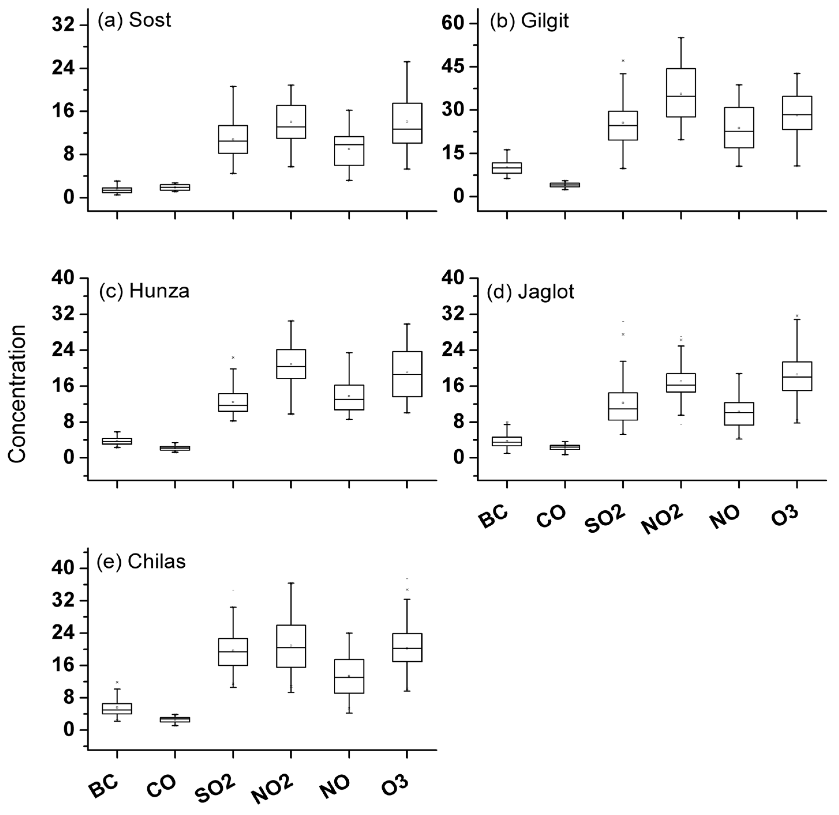
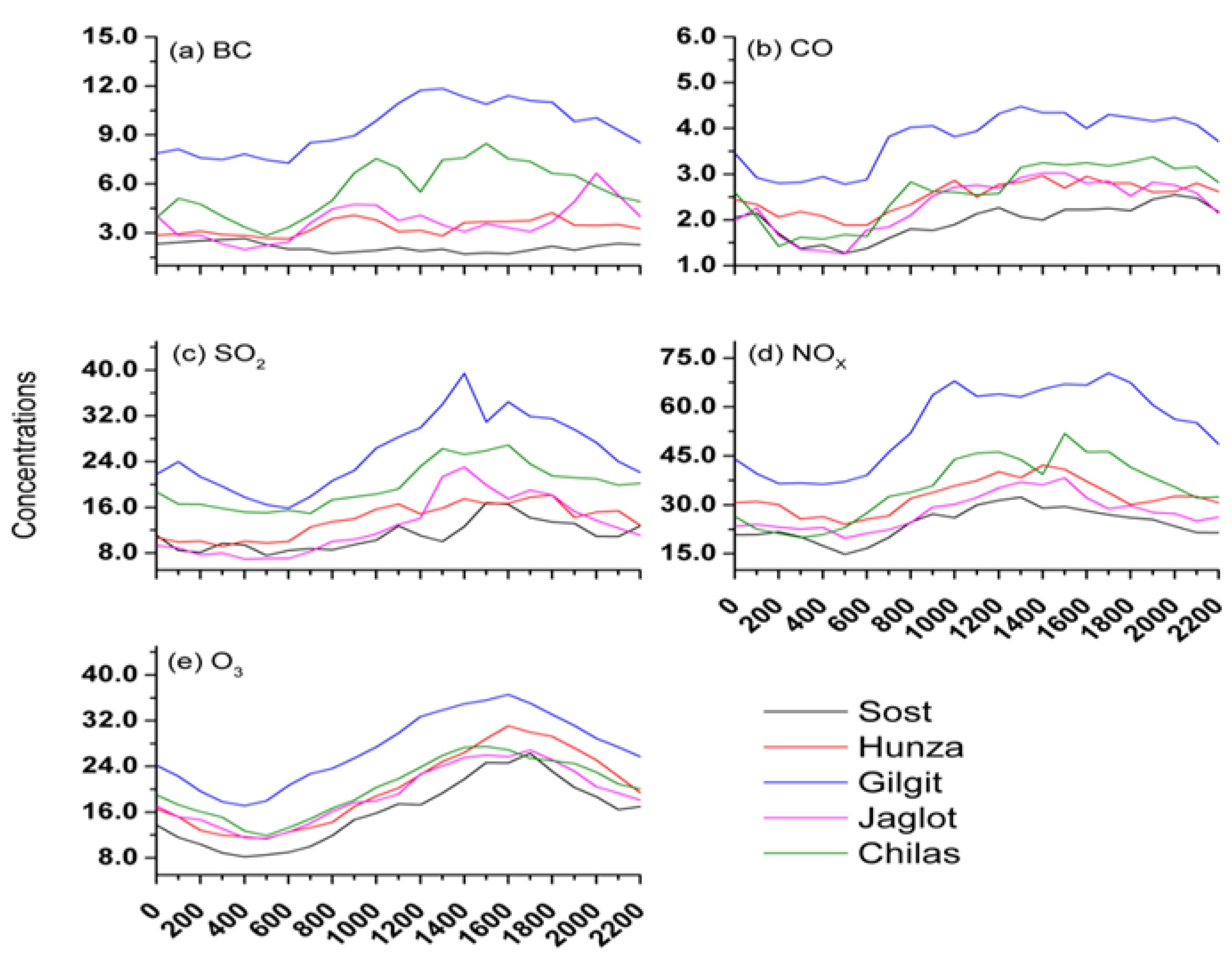
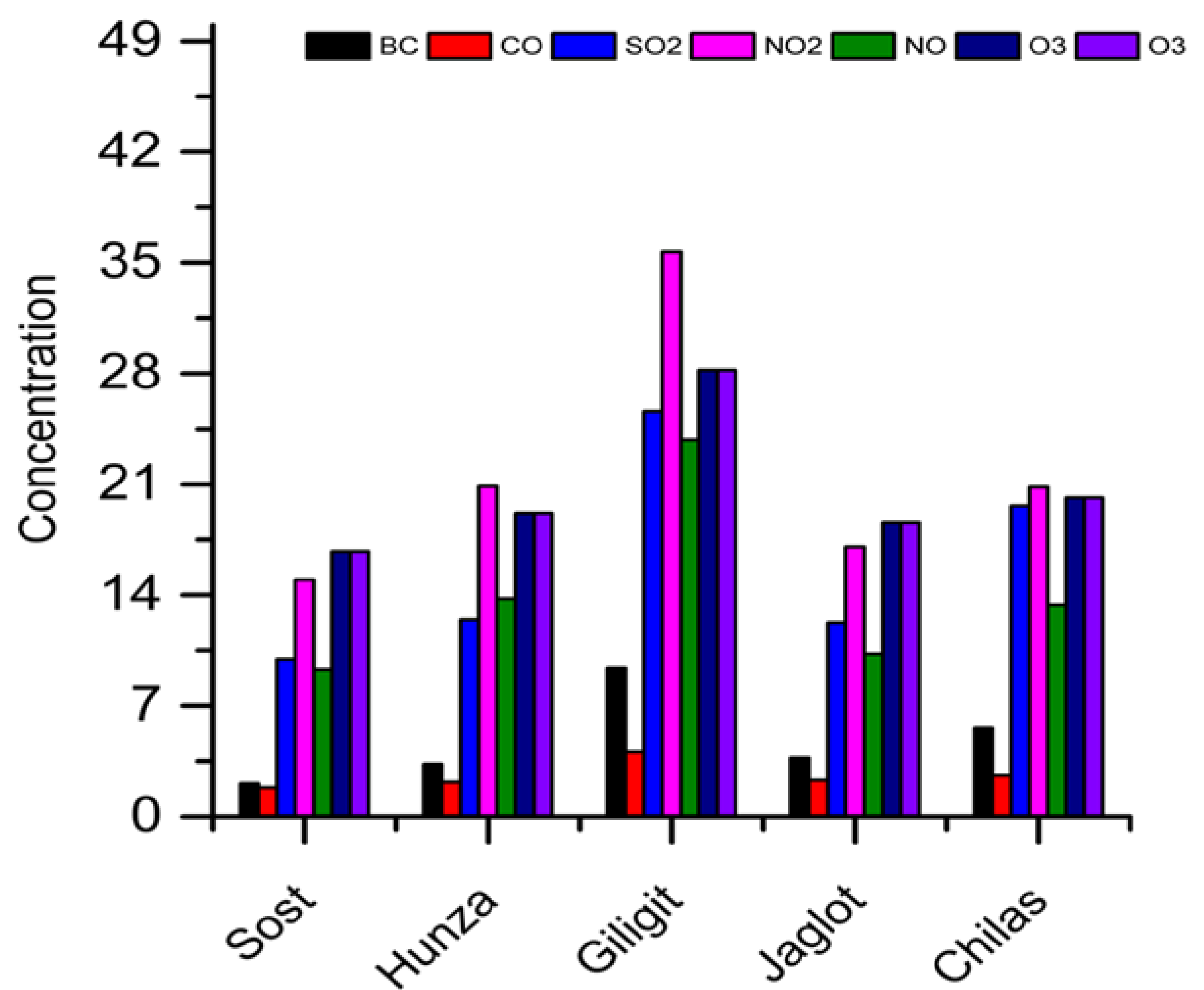
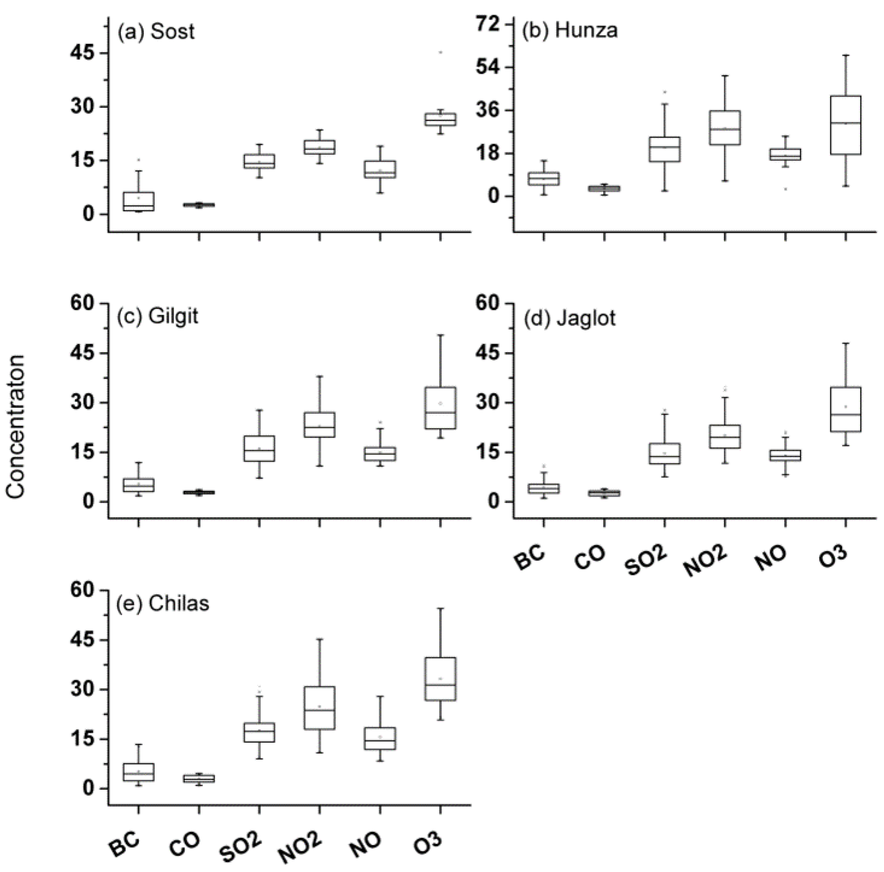
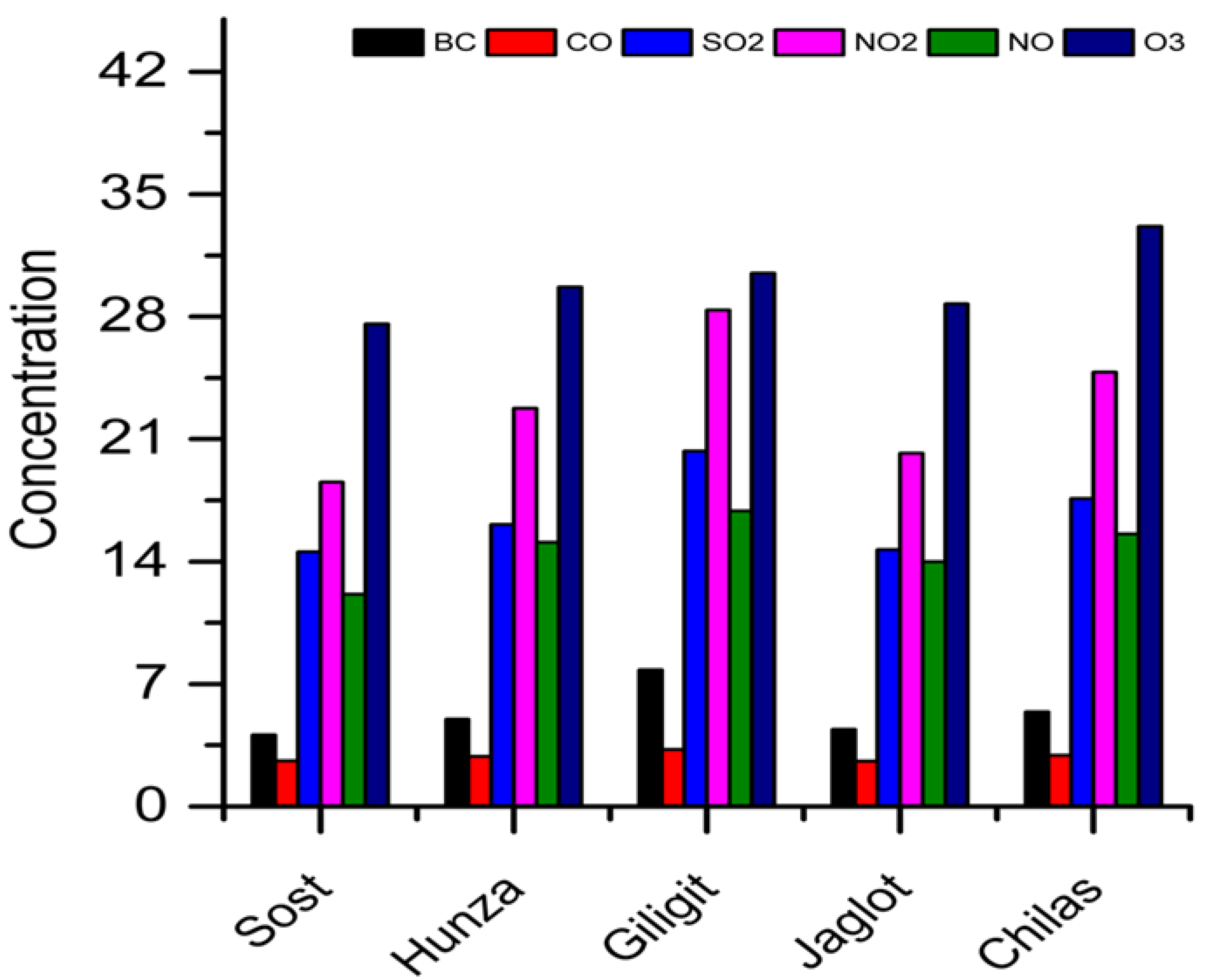
4.1. Spatiotemporal Variation of Air Pollutants

Current study mainly focuses on the determination of PM_2.5, BC, CO, SO₂, NO_X and O₃ concentrations and their associated effects on air quality. Research has illustrated that the concentrations of these analytes are minimal in winter and high in summer.

4.1.1. Variations in PM_2.5 Concentrations

The main criterion for assessments of air quality is the quantification of PM_2.5. In winter, 24 h continuous sampling of PM_2.5 was carried out on daily basis. As shown in

Table 2. Concentrations of selected air pollutants in GB cities during winter, 2019.

Parameters			Sost			Hunza			Gilgit			Jaglot			Chilas
	WHO	NEQS	Min	Max	Avg	Min	Max	Avg	Min	Max	Avg	Min	Max	Avg	Min	Max	Avg
* PM2.5 (µg/m3)	15	35	-	-	25.4	-	-	34.2	-	-	60.1	-	-	29.3	-	-	48.8
BC (µg/m3)			1.7	3.7	2.6	2.3	5.8	3.7	6.3	16.2	10.1	1.0	8.1	3.7	2.2	11.8	5.5
CO (mg/m3)	4	5	0.7	2.9	1.9	1.3	3.5	2.4	1.8	5.5	3.7	0.6	3.5	2.2	1.0	3.8	2.5
SO2 (µg/m3)	40	120	4.5	20.6	11.1	8.1	24.7	13.4	9.8	47.0	25.2	5.1	30.4	12.2	10.5	34.4	19.6
NO (µg/m3)		40	3.2	16.2	9.2	7.7	23.4	12.6	10.1	38.7	21.0	4.1	18.8	10.2	4.2	23.9	13.3
NO2 (µg/m3)		80	5.6	20.9	14.5	9.8	30.4	19.4	15.6	55.0	32.8	7.5	27.0	17.0	9.3	36.3	20.8
O3 (µg/m3)	100	130	5.2	30.6	15.8	8.8	36.9	19.4	10.1	42.7	27.0	7.7	31.7	18.6	9.6	37.3	20.1

* The minimum and maximum values of PM_2.5 are missing during winter because sampling was performed on a 24 h basis, while in summer, it was on a 12 h basis.

, the highest average peak concentrations were observed at Gilgit (60.1 µg/m³), followed by Chilas (48.8 µg/m³), Hunza (34.20 µg/m³) and Jaglot (29.3 µg/m³), while the lowest values were recorded in Sost (25.4 µg/m³). In this season, the 24 h average values were found to be below the NEQS standard (35 µg/m³) at all locations except for Gilgit and Chilas. In contrast to NEQS, these values significantly exceeded the WHO limits (15 µg/m³), i.e., 3.8 times at Gilgit, 2.7 times Chilas, 2 times at Jaglot, 1.7 times at Hunza and 1.3 times at Sost. These elevated concentrations of PM_2.5 may have been due to increased biomass burning from residential heating and cooking purposes in winter [30]. Due to low temperature inversion, particulates are trapped in the lower atmospheric volume. In summer, sampling of PM_2.5 was conducted twice every 24 h, i.e., for 12 h, from 6:00 am to 6:00 pm and for 12 h from 6:00 pm to 6:00 am. During the daytime, the average levels were found to be above 35 μg/m³ in Chilas (52.9 μg/m³), Jaglot (48.9 μg/m³), Hunza (48.7 μg/m³), Gilgit (46.8 μg/m³) and Sost (35.0 μg/m³). These values exceeded the WHO standards by 3.5 times at Chilas, 3.2 times at both Jaglot and Hunza and 3.1 times at Gilgit (see

Table 3. Concentrations of selected air pollutants in GB cities during summer, 2020.

Parameters			Sost			Hunza			Gilgit			Jaglot			Chilas
	WHO	NEQS	Min	Max	Avg	Min	Max	Avg	Min	Max	Avg	Min	Max	Avg	Min	Max	Avg
PM2.5 (µg/m3)	15	35	31.4	39.0	35.0	45.0	52.4	48.7	41.9	51.8	46.8	41.9	55.9	48.9	54.6	63.9	52.9
BC (µg/m3)			0.6	16.2	4.1	1.84	11.9	4.8	0.6	19.8	7.8	1.1	11.3	4.2	0.8	13.4	5.21
CO (mg/m3)	4	5	0.8	3.2	2.3	1.5	3.6	2.7	0.5	5.1	3.2	1.2	3.9	2.6	1.0	4.6	2.9
SO2 (µg/m3)	40	120	4.8	21.4	13.5	6.7	27.7	16.3	2.3	43.7	22.8	7.6	27.8	14.6	9.0	30.9	17.6
NO (µg/m3)		40	5.8	19.0	12.0	9.8	24.1	14.2	3.1	29.8	17.6	7.6	21.5	14.0	8.3	27.9	15.5
NO2 (µg/m3)		80	8.8	25.4	17.9	10.9	38.4	22.2	6.5	50.5	28.1	11.7	34.8	20.1	10.9	45.2	24.8
O3 (µg/m3)	100	130	13.9	45.2	26.9	19.3	50.4	30.0	4.3	59.1	31.4	17.1	48.0	28.7	20.8	54.5	33.1

).

In comparison, the increasing mass concentration in summer could be attributed to road activities, heavy traffic and high wind speeds, which cause mass particles to loft upward. According to [31], major causes of PM_2.5 accumulations may be industrial emissions, vehicle exhausts and dust. The changing concentrations of PM are related to the presence of other analytes. For example, the sources of PM_2.5 may also be responsible for the presence of sulfur and NO_X, which are consequently converted into PM_2.5. SO₂ and NO are considered to be precursors which vary with the varying concentrations of PM_2.5. In addition, while CO is not directly related to PM_2.5, spatially, it has shown similar trends. Increased concentrations of O₃ may trigger the formation of secondary particles through atmospheric oxidation conditions, which will enhance the concentrations of PM_2.5. The concentration of O₃ may be associated with changes in the concentrations of NO_X and PM_2.5. During the COVID-19 lockdown, non-significant changes were observed in the concentrations of PM_2.5 and the other pollutants, as limitations on road and infrastructure activities led to increase indoor and biomass burning [32]. Finally, the role of meteorological conditions cannot be ignored; variations in PM_2.5 concentrations were associated with high humidity, low wind speed, lower temperatures and the associated inversion layer.

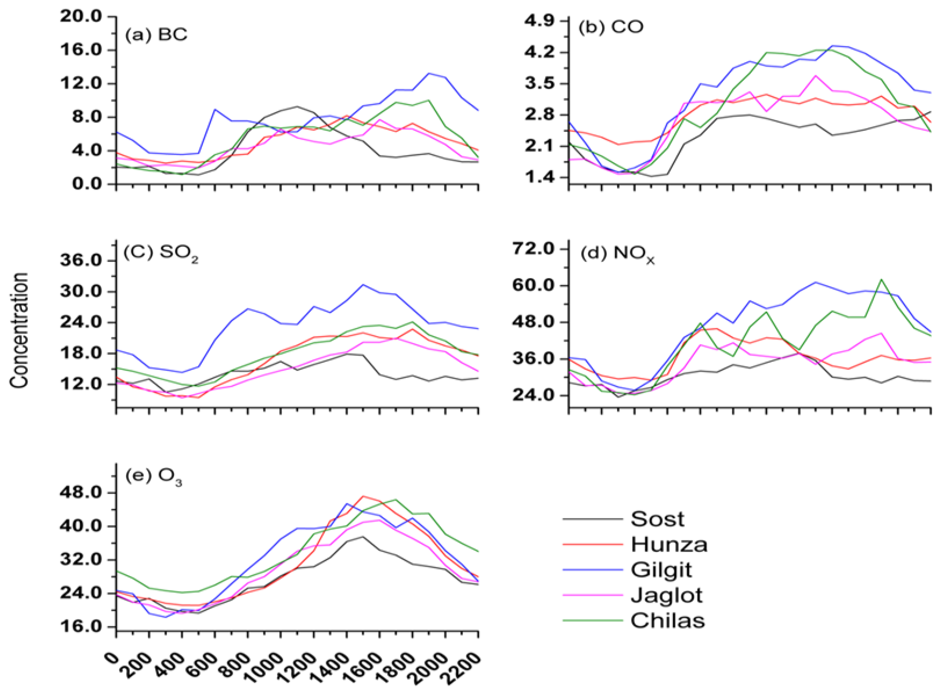
4.1.2. Variations in BC Concentrations

In winter, the average atmospheric values of BC in Sost, Hunza, Gilgit, Jaglot and Chilas ranged from 2.11 to 9.40 µg/m³ (see Figure 2). However, maximum values were found up to 16.2 µg/m³ (at Gilgit); Table 2. Different temporal variations at different study locations with their associated air quality are shown in Figure 3a and Figure 4. Similarly, the average atmospheric values of BC in summer ranged from 4.11 to 7.83 µg/m³ in the five cities, with the maximum value of 19.89 µg/m³ at Gilgit; see Figure 5 and Table 3. In Sost, the diurnal variations of BC concentrations illustrate instantaneous increases by 2–3 times in the morning (7:00 am to 11:00 am) as compared to summer nighttime values at all locations; see Figure 6a. During this period, heavy-duty diesel vehicles stationed at the Sost dry port are started. In Sost, when the Pakistan-China border was open and road activities were maximal, the concentration of BC also rose in the summer. The emission of BC is attributed to the incomplete or inefficient combustion of wood and coal; it therefore tends to come from local urban areas. In winter, this trend was not observed due to insubstantial road activities; however, higher concentrations of BC were observed at night, probably due to household burning activities.

Figure 4 and Figure 7 illustrate that the maximum concentrations of BC were found at Gilgit in both seasons, i.e., 3.2 times higher than the WHO guidelines and 1.5 times higher than the summer values set out by the UK Black Carbon Network for roadside locations [33]. However, there are no specific guidelines in the NEQS for BC values. In general, the summer concentrations of BC were low compared to those in winter. This was attributed to the higher wind speeds, i.e., due to the high temperature inversion layer, particles are dispersed and lofted high in the atmosphere. Details about the observed meteorological conditions are given in

Table 4. Meteorological conditions at the study locations during the winter and summer seasons.

	Winter Season 2019				Summer Season 2020
City	T (°C)	H (%)	WS (m/s)	Wind Direction	T (°C)	H (%)	WS (m/s)	Wind Direction
Sost	−0.8	80.2	Calm-5.7	NW & NE	21.9	33.9	0.5 to 4.5	NW & SE
Hunza	0.4	78.3	Calm-4.5	NW & SE	22.2	36.5	0.5 to 2.0	SW & NW
Gilgit	2.0	74.8	Calm-2.4	NW & S	22.8	59.3	0.4 to 4.0	NW & SW
Jaglot	4.8	70.3	Calm-2.1	NW & S	21.4	57.8	0.4 to 4.0	NW & SE
Chilas	6.4	69.8	Calm-1.9	NW & SE	23.7	52.6	0.4 to 2.0	NW & SW

.

4.1.3. Variations in CO Concentrations

Based on average daily sampling, Figure 2 illustrates different concentrations ranges of CO at the selected locations. In winter, the overall average atmospheric concentrations of CO in Sost, Hunza, Gilgit, Jaglot and Chilas were in the range of 1.97 to 3.75 mg/m³ which is within the permissible limits of the NEQS (5 mg/m³) and WHO (4 mg/m³).

In winter, the maximum concentration of CO, i.e., 5.1 mg/m³ at City Park near Gilgit Airport, matching the NEQS limit and exceeding the WHO standards by 1.3 times in the afternoon and at night. However, this increase was not observed for more than two consecutive hours. High concentrations of CO were observed in the evening and nighttime; see Figure 3b and Table 2. In summer, overall average atmospheric concentrations of CO in all cities were in the range of 2.33 to 3.21 mg/m³, i.e., within permissible limits, although they slightly exceeded the NEQS (5.1 mg/m³) and WHO standards in Gilgit; see Figure 5. The Gilgit station detected a maximum concentration of CO that was beyond the NEQS limit, but not for more than 1 h during summer; see Figure 6b and Table 3. In general, the high mean concentrations of CO may have been due to an increased influx of vehicles and traffic. Being an intermediate product of vehicle and combustion activities emissions, it may not directly impact PM_2.5 levels. Different wind cycles in the winter and summer according to the altitude and the terrain also affect the CO concentrations in the study area [34].

The varying concentrations of CO may be linked to its origins and different meteorological conditions at a local level [6].

4.1.4. Variations in SO₂ Concentrations

In winter, the hourly averaged mass concentrations of SO₂ ranged between 11.17 µg/m³ and 25.28 µg/m³ at all study locations; see Figure 2. These values were found to be within the permissible limits of the NEQS (120 µg/m³) and WHO (40 µg/m³); see Table 2. In summer, the average atmospheric values of SO₂ were found to be between 13.95 µg/m³ to 22.85 µg/m³, i.e., within the permissible limits of the NEQS and WHO; see Figure 5 and Table 3. The maximum concentrations of SO₂ also remained below the NEQS and WHO recommended limits; however, it is interesting to note that higher concentrations of SO₂ were mostly observed during late afternoon or early in the morning, as shown in the diurnal graphs of SO₂ for all study sites; see Figure 3c and Figure 6c,f. The concentrations of SO₂ are considered as an important indicator for the formation of PM_2.5; therefore, similar trends were found in both seasons. This rise could have been due to household burning of coal for heating purposes in winter, as well as thermal inversion phenomena in winter.

4.1.5. Variation in NO and NO₂ Concentrations

In this study, the term nitrogen oxides is being used to include for nitric oxide and nitrogen dioxide (NO_X). NO is considered as a major air pollutant, but there are no reference data or standard limits for it, as it rapidly oxidizes with oxygen in ambient conditions to form NO₂. In winter, the average atmospheric values ranged between 9.23 and 21.02 µg/m³ in Sost, Hunza, Gilgit, Jaglot and Chilas, i.e., within permissible limits of the NEQS (40 µg/m³). No specific limits are cited by the WHO; see Figure 2. The same figure shows that for NO₂, the average atmospheric values in all cities were between 14.53 µg/m³ and 32.80 µg/m³, i.e., within the NEQS limit of 80 µg/m³ but exceeding the WHO value (25 µg/m³) by 1.2 times at Gilgit in winter; see Table 2.

The concentrations of NO₂ showed maximum values of 30.4 µg/m³ at Hunza, 55 µg/m³ at Gilgit and 36 µg/m³ at Chilas in winter; see Table 2. The same behavior was found for Gilgit in summer, with maximum values of 38.4 µg/m³ at Hunza, 50.5 µg/m³ at Gilgit, 34.8 µg/m³ at Jaglot and 45.2 µg/m³ at Chilas, exceeding the WHO limits; see Table 3. Similarly, in summer, the overall average concentrations of NO were between 12.40 and 17.68 µg/m³ in all selected cities, i.e., within the NEQS limit (40 µg/m³); see Figure 5. On the other hand, the overall average values of NO₂ (17.95 to 28.18 µg/m³) in all cities also reached the NEQS limits; see Table 3. During combustion, a mixture of NO₂ and NO (e.g., NOx) is formed at high temperatures by the oxidation of nitrogen in fuel. Like SO₂, nitrogen oxides may also effectively affect the concentrations of PM_2.5. As such, high concentrations can be found across the CPEC Route.

As there are no specific WHO guidelines for NO, this study focused on the combined effect of NO and NO₂. The average diurnal variation of NO_X (see Figure 3d and Figure 6d) depicts an increasing trend in the afternoon. The main anthropogenic sources of nitrogen oxides are road transport, gas heaters, and industrial boilers. High concentrations can be found, especially near busy roads and indoor environments [35,36]. The maximum concentrations of NOx were observed in Gilgit in both seasons; see Figures S1 and S2. These concentrations can contribute to the development of acute or chronic bronchitis [36]. NOx acts mainly as an irritant, affecting the mucus membranes of eyes, nose, throat, and respiratory tract.

4.1.6. Variation in O₃ Concentrations

In winter, the average hourly mass concentrations of O₃ ranged between 15.86 and 27.02 μg/m³ (see Figure 2), while in summer, they ranged between 26.33 and 33.16 μg/m³ (see Figure 5). In both seasons, these values were within the permissible limits of the NEQS (130 μg/m³) and WHO (100 μg/m³); see Table 2 and Table 3. An increasing trend was observed in the afternoon in both seasons; see Figure 3e and Figure 6e. However, in this study, O₃ concentrations showed variations in both seasons at different locations (see Figures S1 and S2). The decrease (increase) in winter (summer) was due to the relatively lower and more intense radiations, respectively. Generally, increased solar radiation supports the photochemical production of surface O₃ in such periods. As such, it is considered a secondary pollutant which is produced photo-chemically in the troposphere by its precursors i.e., nitrogen oxides and CO, which are emitted by vehicles along CPEC. The decreasing trend of O₃ and its precursors may be linked to variations in the concentrations of NO_X, VOC, and meteorological conditions. These effects are caused by the reduced daylight duration and solar radiation. In contrast, enhanced photochemical oxidation of O₃ and its precursors occurs with long daylight duration and intense solar radiation [37]. As such, the increased temperature in the northern part of Pakistan during summer leads to an increase in O₃. Comparatively, the subtle increase in O₃ observed in summer during the COVID-19 pandemic suggests little effect on the mitigation of air pollution [32].

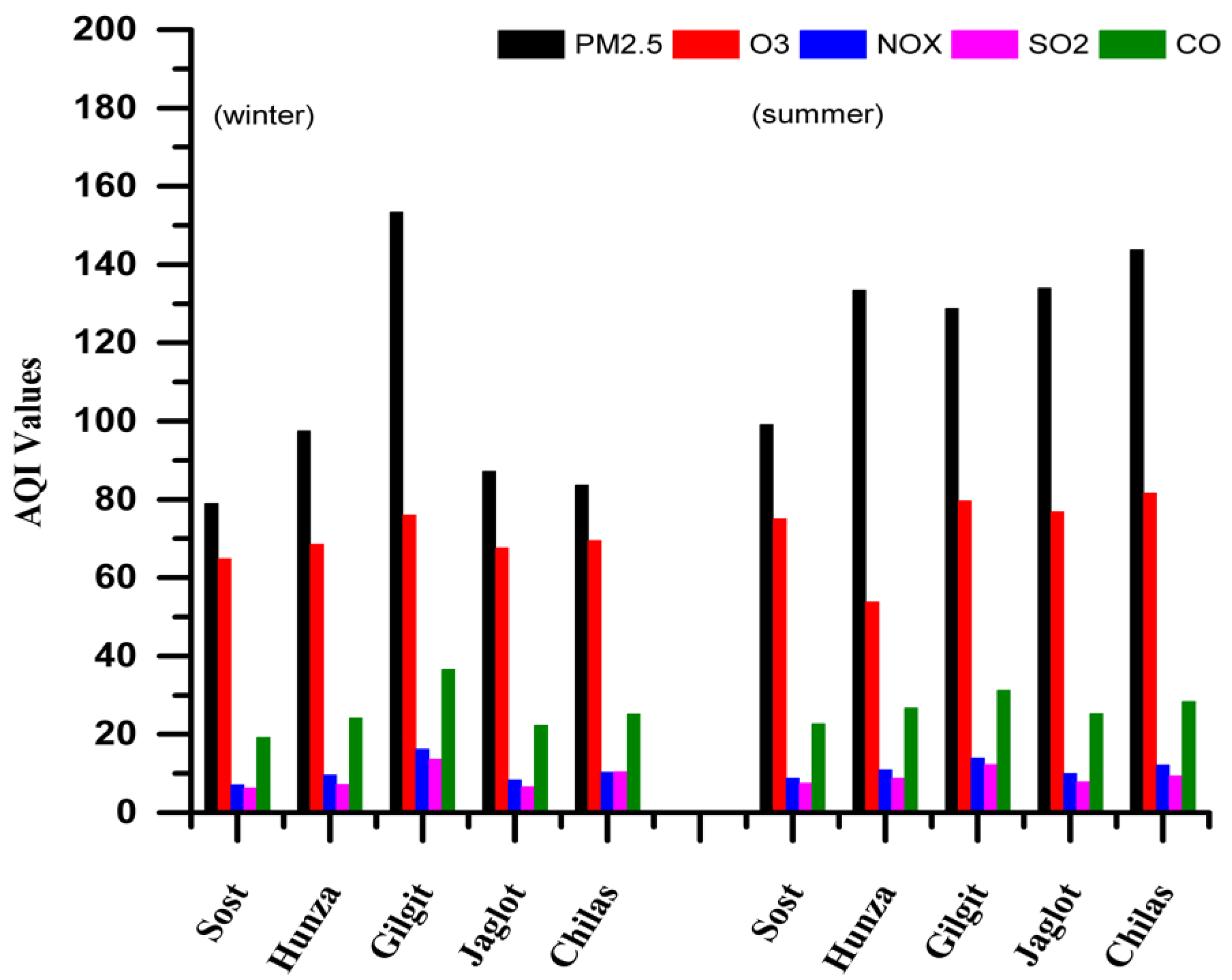
4.2. Air Quality Assessment

Air quality indices (AQI) can be used to assess air quality and its short-term implications. Higher values of AQI indicate high levels of air pollution. Based on Equations (1)–(3), the AQI were calculated for Sost, Hunza, Gilgit, Jaglot, and Chilas during winter 2019 and summer 2020. The AQI standard for each pollutant was based on the WHO standard limits. Additionally, these values were compared with rating scales [38,39]. The highest values, especially those of PM_2.5 and CO, were observed at Gilgit. Overall, high levels of air pollutants were observed in summer in other cities. A seasonal comparison showed that higher pollutant levels were observed in Gilgit and Chilas in winter than in summer, whereas in other cities i.e., Hunza, Jaglot and Sost, overall higher pollutant levels were observed in summer than in winter.

The dry weather conditions and frequent inversion layers during winter, together with traffic congestion in populated areas and the burning of wood or other fuel for heating purposes, resulted in a relatively higher pollution load in Gilgit and Chilas. PM_2.5 value which are considered unhealthy for sensitive groups were observed at Gilgit (60.1 μg/m³) and Chilas (48.8 μg/m³) in winter, while moderate levels were observed at Sost, Hunza and Jaglot during winter, 2019. For these peaks, the AQI values are given

Table 5. AQI values for selected analytes in winter, 2019.

No.	Station	PM2.5	O3	NOX	SO2	CO
1	Sost	79.0	64.9	7.1	6.3	19.2
2	Hunza	97.5	68.6	9.6	7.2	24.2
3	Gilgit	153.4 *	76.0	16.2	13.6	36.6
4	Jaglot	87.2	67.7	8.4	6.6	22.3
5	Chilas	83.7	69.5	10.3	10.4	25.2

Values with “*” in Table 5 and Table 6 represent unhealthy levels of air pollutants.

. An AQI value in the range of 151–200 is considered unhealthy.

However, in summer, unhealthy levels were observed at Hunza (48.7 μg/m³), Gilgit (46.8 μg/m³⁾, Jaglot (48.9 μg/m³) and Chilas (52.9 μg/m³); the AQI values are given in

Table 6. AQI values for selected analytes in summer, 2020.

S. No.	Station	PM2.5	O3	NOX	SO2	CO
1	Sost	99.2	75.1	8.8	7.5	22.7
2	Hunza	133.5 *	53.8	11.0	8.8	26.8
3	Gilgit	128.8 *	79.7	13.9	12.3	31.3
4	Jaglot	134.0 *	76.9	10.0	7.9	25.3
5	Chilas	143.8 *	81.6	12.2	9.4	28.4

Values with “*” in Table 5 and Table 6 represent unhealthy levels of air pollutants.

. There are no specific guidelines for BC from the NEQS or WHO; however, the WHO uses some specific values from the UK Black Carbon Network. Based on the BC datasets, the study area was found to be unsafe for most of both seasons. PM_2.5 has been noted as dominating pollutant compared to gaseous pollutants, which is alarming and underlines the need for continuous monitoring at critical locations. Based on the AQI and average hourly sampling of CO, good and acceptable values, i.e., in the range of 0–50, were observed at all study locations; however, unsafe levels were detected at different times at Gilgit in the winter [6]. Similar observations were made in the summer. SO₂ affects plants and animals; concentrations of this compound in the range of 0–35 are considered to be satisfactory. The SO₂ in the atmosphere is mainly caused by industrial activities and fuel consumption. In both seasons, the AQI values for NO_X in the range of 0–53 were considered good. Therefore, in the present study, it was found that NO_X poses no major threat to air quality. AQI values for O₃ in the range of 50–100 are considered to be moderate; however, certain people should take precautionary measures when performing physical activities outdoors. In summer, the increase in ozone concentration may adversely affect human health [40,41]. Comparatively, high AQI values were observed for PM_2.5 and O₃ in summer 2020, while other analytes showed uneven distribution among the study sites; see Figure 8.

Overall, based on air quality indices, concentrations of SO₂, NO_X and O₃ were found to be within the NEQS and WHO limits, with good and satisfactory conditions in both seasons at all study locations.

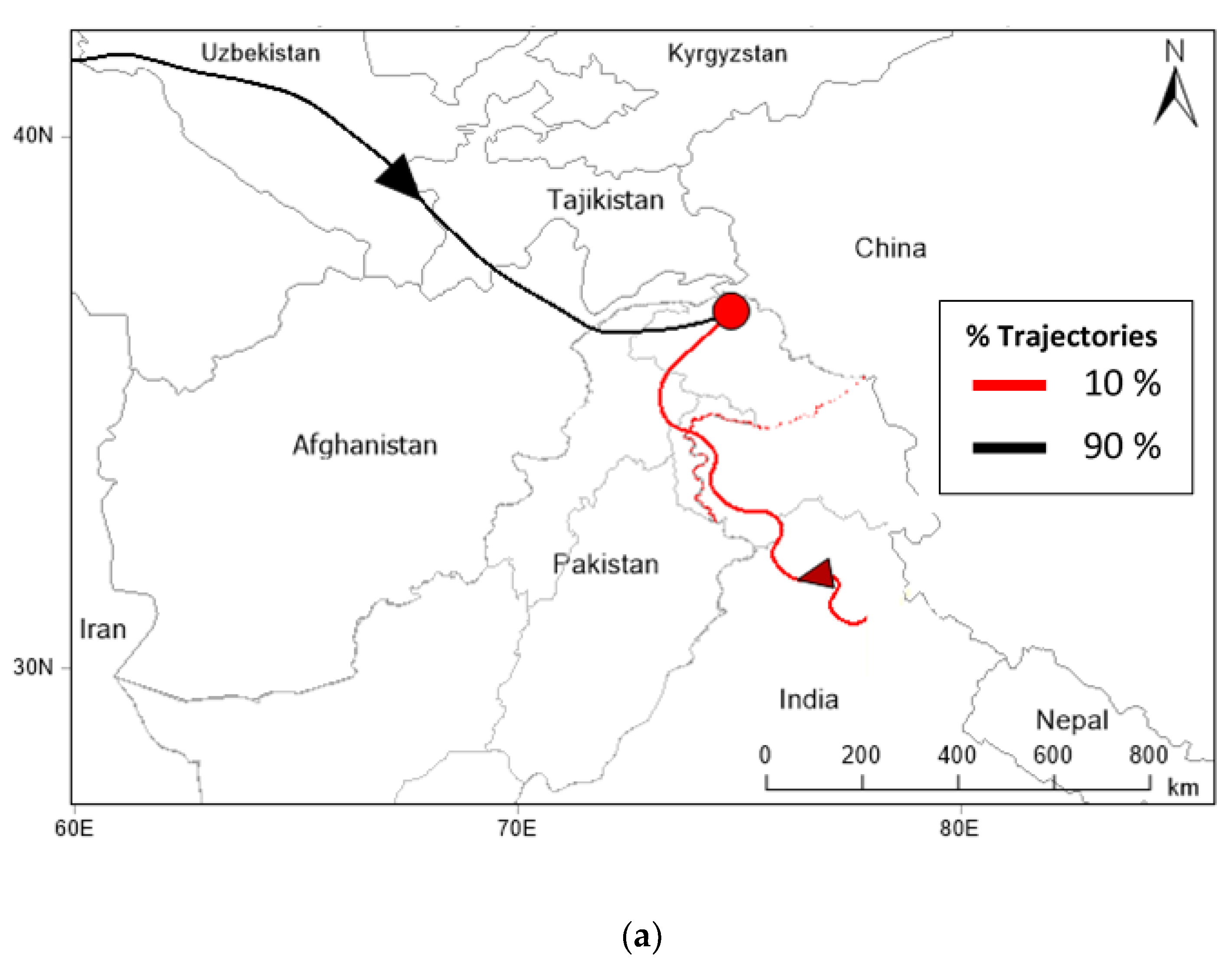
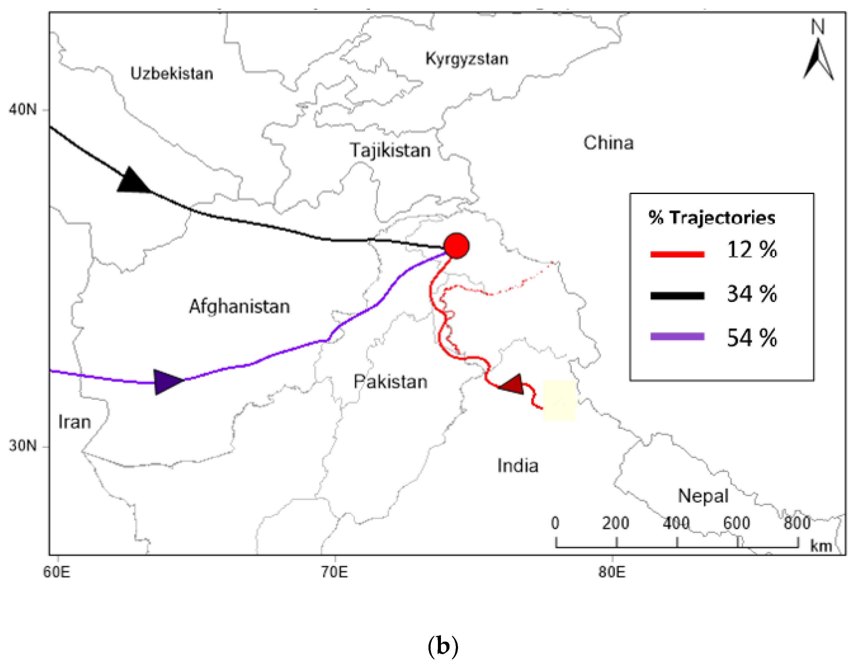
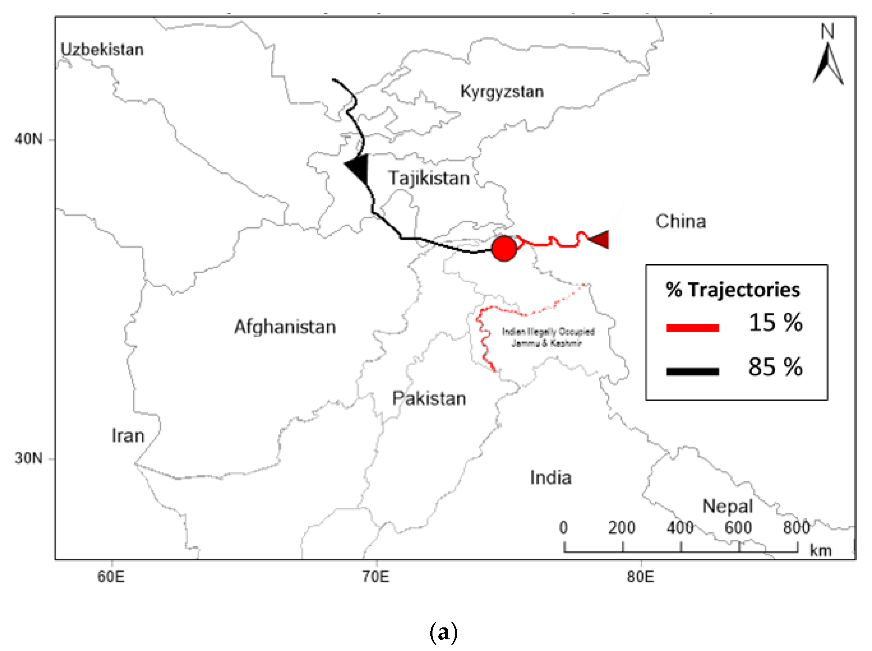
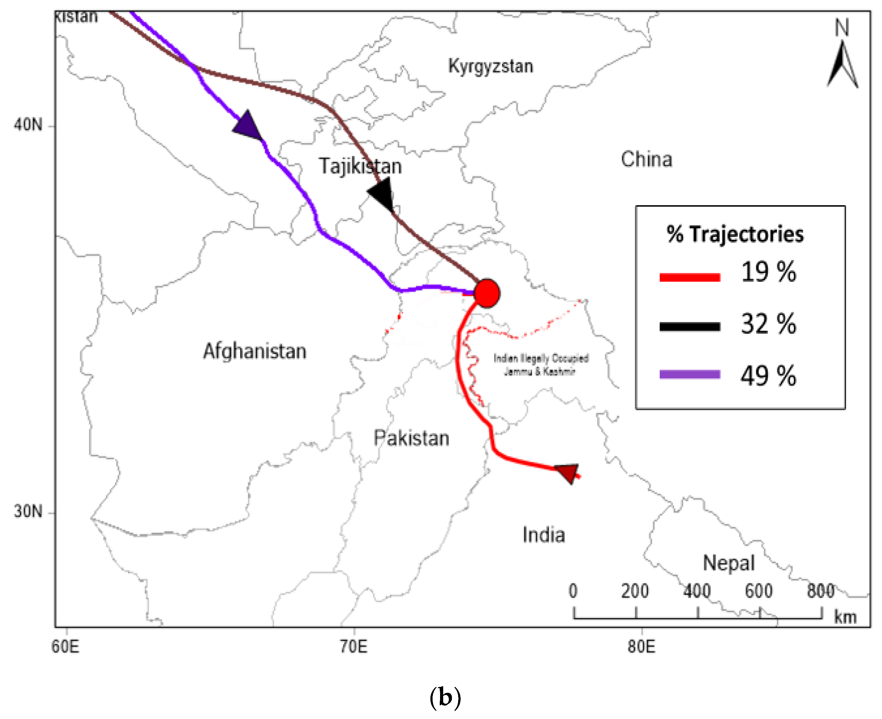
4.3. Influence of Air Masses on Air Pollutants

Figure 9a,b illustrates that the major fraction of received air masses originated primarily from the Black Sea or Caspian Sea regions and traveled over Eastern Europe and central Asia. Regions of the Mediterranean Sea and Middle East were secondary sources of westerlies passing over Iran, Afghanistan and Pakistan before reaching the study sites in Gilgit-Baltistan except Sost, the northernmost part of Gilgit-Baltistan. The major source of pollutants at the study sites could be the fractions of eastern winds originating from northern India or the central region of Pakistan that could also carry smoke from household burning and vehicular emissions. Figure 10a,b illustrates that during summer, in Sost, the major fraction of air masses arrived from central Asia, whereas minor fractions from China also intruded. Elsewhere in the study region i.e., Hunza, Gilgit, Jaglot and Chilas, the major fraction of air masses originated primarily from the Black Sea or Caspian Sea regions and traveled over Eastern Europe and central Asia. The secondary source of pollutants to all monitoring sites except Sost was likely easterly winds originating over northern India that carried emissions from household burning and vehicular emissions. Figure 11 presents the average (day/night) wind speed and wind direction in Sost, Hunza, Gilgit, Jaglot and Chilas in the summer and winter seasons. During the study period, in all cities, low speed winds (0.1 to 5 m/s) prevailed. For the wind class frequency distribution at each study site, see Figure S3. Most of the winds at the study sites came from northwest and southwest directions, followed by southeast. The “wind rose” method can be used to track the influence of local wind (i.e., originating in the last 2 or 3 h before reaching the station), but in the longer term, its data can be misleading. For example, valley winds in mountainous regions can be different to the general circulation and the synoptic scale wind-field [42]. The general weakness of using wind roses is that one cannot assume that the wind direction measured at a point is consistent with the synoptic scale flow. The turbulent and synoptic nature of wind always leads to changes in wind direction over a region, and this is not shown from local or point wind direction measurements. To overcome this gap, Hybrid Single-Particle Lagrangian Integrated Trajectory Model (HYSPLIT) was used in the present study.

5. Conclusions

Using field measurements of CO, SO₂, NOx (NO/NO₂), O₃ and aerosol pollutants including BC and PM_2.5 concentrations near and along the CPEC Route, this study focused on minute scale variations in the concentrations of these pollutants. It is the first study of its kind, providing insights into dynamic variations at five sites in the glaciated region of northern Pakistan during winter (2019) and summer (2020). Significant insights into air quality and the seasonal variation of major pollutant levels, taking into account associated local and transboundary air masses, was presented. The baseline data in the Atlas provide comprehensive information of present trends and can serve as a reference to examine future changes in the ecosystem of Gilgit-Baltistan. The highest values of all pollutants were recorded in Gilgit city, particularly in the vicinity of City Park and the airport. Maximum concentrations of selected analytes of all pollutants were below NEQS limits, except for CO, which exceeded the guideline values during peak traffic hours. In summer, the average atmospheric concentrations of gaseous pollutants (CO, SO₂, NO, NO₂ and O₃) in all selected cities were also found to be within limits of NEQS. Like in winter, higher values of all pollutants were recorded around Gilgit City Park and Airport, where maximum concentrations of CO, i.e., slightly higher than standard limit, were recorded during peak traffic hours. In general, the atmospheric concentrations (day/night) of PM_2.5 in all cities met the NEQS guidelines (for 24 h); however, this was not the case in Gilgit and Chilas. In our seasonal comparison, it was found that in winter, higher values of air pollutants were present in Gilgit and Chilas than in summer, whereas in other cities, i.e., Hunza, Jaglot and Sost, overall higher values were observed in summer. Although BC aerosols are not listed as pollutants and, as such, no NEQS guidelines exist for them, these aerosols have recently have received a great deal of attention due to their strong ability to absorbing sunlight. This database may be used to compare their atmospheric concentrations during the post-operational phase of CPEC, as well as in mathematical simulations to estimate atmospheric warming and its impact on snow albedo in the future. Local and transboundary emissions can have profound effects on the concentrations of gaseous and aerosol pollutants. In order to make informed environmental management decisions and to take timely and effective measures to control anthropogenic emissions in GB during the operational phase of CPEC, the following technical/administrative actions are recommended:

• Permanent air quality monitoring stations should be established at critical locations along the CPEC in GB for year-round monitoring of gaseous and aerosol pollutants. The collected data should be disseminated to an atmosphere knowledge hub that may be established at GB-EPA to develop the air pollution database.
• A GIS-based emission inventory of air pollutants from mobile and stationary sources should be developed and integrated with computer modeling and satellite data to identify pollutant sources and forecast future emission loads in GB.
• The GB government should adopt its own air emission standards, keeping in view the local situation and ecosystem.
• District-wise studies should be initiated in collaboration with research organizations and universities on the sources of pollutants and their impacts on health, the ecosystem and the economy.

References

1. Maleki, H.; Sorooshian, A.; Alam, K.; Fathi, A.; Weckwerth, T.; Moazed, H.; Jamshidi, A.; Babaei, A.A.; Hamid, V.; Soltani, F.; et al. The impact of meteorological parameters on PM10 and visibility during the Middle Eastern dust storms. J. Environ. Health Sci. Eng. 2022, 20, 495–507. [Google Scholar] [CrossRef] [PubMed]
2. WHO. 9 out of 10 People Worldwide Breathe Polluted Air, but More Countries Are Taking Action; WHO: Geneva, Switzerland, 2018. [Google Scholar]
3. Farsani, M.H.; Shirmardi, M.; Alavi, N.; Maleki, H.; Sorooshian, A.; Babaei, A.; Asgharnia, H.; Marzouni, M.B.; Goudarzi, G. Evaluation of the relationship between PM10 concentrations and heavy metals during normal and dusty days in Ahvaz, Iran. Aeolian Res. 2018, 33, 12–22. [Google Scholar] [CrossRef]
4. Mannucci, P.M.; Franchini, M. Health effects of ambient air pollution in developing countries. Int. J. Environ. Res. Public Health 2017, 14, 1048. [Google Scholar] [CrossRef]
5. Bari, M.A.; Kindzierski, W.B. Concentrations, sources and human health risk of inhalation exposure to air toxics in Edmonton, Canada. Chemosphere 2017, 173, 160–171. [Google Scholar] [CrossRef] [PubMed]
6. Wang, Y.; Zhao, M.; Han, Y.; Zhou, J. A fuzzy expression way for air quality index with more comprehensive information. Sustainability 2017, 9, 83. [Google Scholar] [CrossRef] [Green Version]
7. Monks, P.S.; Granier, C.; Fuzzi, S. Atmospheric composition change-global and regional air quality. Atmos. Environ. 2009, 43, 5268–5350. [Google Scholar]
8. Isaksen, I.S.A.; Granier, C.; Myhre, G.; Berntsen, T.; Dalsøren, S.B.; Gauss, M.; Klimont, Z.; Benestad, R.; Bousquet, P.; Collins, T. Chapter 12-Atmospheric Composition Change: Climate–Chemistry Interactions. In The Future of the World’s Climate, 2nd ed.; Ann, H.-S., Kendal, M., Eds.; Elsevier: Boston, MA, USA, 2012; pp. 309–365. [Google Scholar]
9. He, H.D.; Lu, W.Z. Urban aerosol particulates on Hong Kong roadsides: Size distribution and concentration levels with time. Stoch. Environ. Res. Risk Assess. 2012, 26, 177–187. [Google Scholar]
10. Tiwary, A.; Robins, A.; Namdeo, A.; Bell, M. Air flow and concentration fields at urban road intersections for improved understanding of personal exposure. Environ. Int. 2011, 37, 1005–1018. [Google Scholar] [CrossRef] [PubMed]
11. Galatioto, F.; Zito, P. Traffic parameters estimation to predict road side pollutant concentrations using neural networks. Environ. Model. Assess. 2009, 14, 365–374. [Google Scholar] [CrossRef]
12. Lurie, K.; Nayebare, S.R.; Fatmi, Z.; Carpenter, D.O.; Siddique, A.; Malashock, D.; Khan, K.; Zeb, J.; Hussain, M.M.; Khatib, F.; et al. PM2.5 in a Megacity of Asia (Karachi): Source Apportionment and Health Effects. Atmos. Environ. 2019, 202, 223–233. [Google Scholar] [CrossRef]
13. Landrigan, P.J. Air pollution and health. Lancet Pub. Health 2016, 2, e4–e5. [Google Scholar] [CrossRef] [PubMed] [Green Version]
14. Forouzanfar, M.H.; Afshin, A.; Alexander, L.T.; Anderson, H.R.; Bhutta, Z.A. Global, regional, and national comparative risk assessment of 79 behavioral, environmental and occupational, and metabolic risks or clusters of risks, 1990–2015: A systematic analysis for the Global Burden of Disease Study 2015. Lancet 2016, 388, 1659–1724. [Google Scholar] [CrossRef]
15. Wang, P.; Mihaylova, L.; Chakraborty, R.; Munir, S.; Mayfield, M.; Alam, K.; Khokhar, M.F.; Zheng, Z.; Jiang, C.; Fang, H. A Gaussian Process Method with Uncertainty Quantification for Air Quality Monitoring. Atmosphere 2021, 12, 1344. [Google Scholar] [CrossRef]
16. Ahmad, M.; Alam, K.; Tariq, S.; Blaschke, T. Contrasting changes in snow cover and its sensitivity to aerosol optical properties in Hindukush-Karakoram-Himalaya region. Sci. Total Environ. 2020, 699, 134356. [Google Scholar] [CrossRef] [PubMed]
17. Zeb, B.; Alam, K.; Sorooshian, A.; Chishtie, F.; Ahmad, I.; Bibi, H. Temporal characteristics of aerosol optical properties over the glacier region of northern Pakistan. J. Atmos. Sol. Terr. Phys. 2019, 186, 35–46. [Google Scholar] [CrossRef] [PubMed]
18. Ahmad, M.; Alam, K.; Tariq, S.; Anwar, S.; Nasir, J.; Mansha, M. Estimating fine particulate concentration using a combined approach of linear regression and artificial neural network. Atmos. Environ. 2019, 219, 117050. [Google Scholar] [CrossRef]
19. WHO. WHO Global Ambient Air Quality Database (Update 2018); WHO: Geneva, Switzerland, 2018. [Google Scholar]
20. Link, M.F.; Kim, J.; Park, G.; Lee, T.; Park, T.; Babar, Z.B.; Sung, K.; Kim, P.; Kang, S.; Kim, J.S.; et al. Elevated production of NH4NO3 from the photochemical processing of vehicle exhaust: Implications for air quality in the Seoul Metropolitan Region. Atmos. Environ. 2017, 156, 95–101. [Google Scholar] [CrossRef]
21. Health Effects Institute. State of Global Air 2019: A Special Report on Global Exposure to Air Pollution and Its Disease Burden; Health Effects Institute: Boston, MA, USA, 2019. [Google Scholar]
22. Babar, Z.B.; Park, J.H.; Kang, J.; Lim, H.J. Characterization of a smog chamber for studying formation and physicochemical properties of secondary organic aerosol. Aerosol Air Qual. Res. 2016, 16, 3102–3113. [Google Scholar] [CrossRef] [Green Version]
23. Amnesty International. Pakistan: Hazardous Air Puts Lives at Risk. Available online: https://www.amnesty.org/en/latest/news/2019/10/pakistan-hazardous-air/ (accessed on 1 June 2019).
24. UNDP. Sustainable Urbanization. Dev. Advocate Pak. 2019, 5, 4. [Google Scholar]
25. Babar, Z.B.; Park, J.H.; Lim, H.J. Influence of NH3 on secondary organic aerosols from the ozonolysis and photooxidation of α-pinene in a flow reactor. Atmos. Environ. 2017, 164, 71–84. [Google Scholar] [CrossRef]
26. EPA. List of Designated Reference and Equivalent Methods; EPA: Washington, DC, USA, 2016; Volume 17, p. 202016-2.
27. Yazdani, M.; Baboli, Z.; Maleki, H.; Birgani, Y.T.; Zahiri, M.; Chaharmahal, S.S.H.; Goudarzi, M.; Mohammadi, M.J.; Alam, K.; Sorooshian, A.; et al. Contrasting Iran’s air quality improvement during COVID-19 with other global cities. J. Environ. Health Sci. Eng. 2021, 19, 1801–1806. [Google Scholar] [CrossRef]
28. Kassomenos, P.A.; Kelessis, A.; Petrakakis, M.; Zoumakis, N.; Christidis, T.; Paschalidou, A.K. Air quality assessment in a heavily polluted urban Mediterranean environment through air quality indices. Ecol. Indic. 2012, 18, 259–268. [Google Scholar] [CrossRef]
29. Wang, Y.; Zhang, X.; Draxler, R.R. TrajStat: GIS-based software that uses various trajectory statistical analysis methods to identify potential sources from long-term air pollution measurement data. Environ. Model. Softw. 2009, 24, 938–939. [Google Scholar] [CrossRef]
30. Chen, P.; Kang, S.; Yang, J.; Pu, T.; Li, C.; Guo, J.; Tripathee, L. Spatial and temporal variations of gaseous and particulate pollutants in six sites in Tibet, China, during 2016–2017. Aerosol Air Qual. Res. 2019, 19, 516–527. [Google Scholar] [CrossRef] [Green Version]
31. Li, L.; Lin, G.Z.; Liu, H.Z.; Guo, Y.; Ou, C.Q.; Chen, P.Y. Can the Air Pollution Index be used to communicate the health risks of air pollution? Environ. Pollut. 2015, 205, 153–160. [Google Scholar] [CrossRef] [PubMed]
32. Khan, R.; Kumar, K.R.; Zhao, T. The impact of lockdown on air quality in Pakistan during the COVID-19 pandemic inferred from the multi-sensor remote sensed data. Aerosol Air Qual. Res. 2021, 21, 200597. [Google Scholar] [CrossRef]
33. Butterfield, D.; Beccaceci, S.; Quincey, P.; Sweeney, B.; Lilley, A.; Bradshaw, C.; Fuller, G.; Green, D.; Font, A. 2015 Annual Report for the UK Black Carbon Network; (NPL Report ENV7. 17 August 2020); National Physical Laboratory: Teddington, UK, 2016. [Google Scholar]
34. Ur Rehman, S.A.; Cai, Y.; Siyal, Z.A.; Mirjat, N.H.; Fazal, R.; Kashif, S.U.R. Cleaner and sustainable energy production in Pakistan: Lessons learnt from the Pak-TIMES model. Energies 2019, 13, 108. [Google Scholar] [CrossRef] [Green Version]
35. Popescu, F.; Ionel, I. Anthropogenic Air Pollution Sources; Air Quality; Kumar, A., Ed.; Intech: London, UK, 2010; pp. 1–22. [Google Scholar]
36. Theophanides, M.; Anastassopoulou, J.; Theophanides, T. Air Polluted Environment and Health Effects. Indoor and Outdoor Air Pollution. Air Pollut. Environ. Health Eff. 2011, 3–28. [Google Scholar]
37. Liu, H.; Liu, S.; Xue, B.; Lv, Z.; Meng, Z.; Yang, X.; Xue, T.; Yu, Q.; He, K. Ground-level ozone pollution and its health impacts in China. Atmos. Environ. 2018, 173, 223–230. [Google Scholar] [CrossRef]
38. Kumar, G.; Kumar, S. Air quality index. A comparative study for assessing the status of air quality before and after lockdown for Meerut. Mater. Today Proc. 2002, 1, 3497–3500. [Google Scholar] [CrossRef]
39. Kaushik, C.P.; Ravindra, K.; Yadav, K.; Mehta, S.; Haritash, A.K. Assessment of ambient air quality in urban centres of Haryana (India) in relation to different anthropogenic activities and health risks. Environ. Monit. Assess. 2006, 122, 27–40. [Google Scholar] [CrossRef] [PubMed] [Green Version]
40. Kumar, K.R.; Sivakumar, V.; Reddy, R.R.; Gopal, K.R. Ship-borne measurements of columnar and surface aerosol loading over the bay of Bengal during W-ICARB campaign: Role of air mass transport, latitudinal and longitudinal gradients. Aerosol Air Qual. Res. 2013, 13, 818–837. [Google Scholar] [CrossRef]
41. Zhou, T.; Jian, S.; Huan, Y. Temporal and Spatial Patterns of China’s Main Air Pollutants: Years 2014 and 2015. Atmosphere 2017, 8, 137. [Google Scholar] [CrossRef] [Green Version]
42. Fleming, Z.L.; Monks, P.S.; Manning, A.J. Review: Untangling the influence of air-mass history in interpreting observed atmospheric composition. Atmos. Res. 2012, 104, 1–39. [Google Scholar] [CrossRef]
Figure 1. A detailed map of the study area showing Sost, Hunza, Gilgit, Jaglot and Chilas.
Atmosphere 13 01994 g001
Figure 2. Variation in concentration ranges of BC ( μ g/m3), CO (mg/m3), SO2, NO, NO2 and O3 in μ g/m3 at selected sites in Gilgit-Baltistan during winter, 2019.
Atmosphere 13 01994 g002
Figure 3. Diurnal variation of (a) BC (in µg/m3), (b) CO (in mg/m3), (c) SO2 (in µg/m3), (d) NOX (in µg/m3) and (e) O3 (in µg/m3) at selected study sites in Gilgit-Baltistan during winter, 2019.
Atmosphere 13 01994 g003
Figure 4. Daily average air quality indicators at all study sites during winter, 2019.
Atmosphere 13 01994 g004
Figure 5. Variation in concentration ranges of BC ( μ g/m3), CO (mg/m3), SO2, NO, NO2 and O3 in μ g/m3 at selected sites in Gilgit-Baltistan during summer, 2020.
Atmosphere 13 01994 g005
Figure 6. Diurnal variation of (a) BC (in µg/m3), (b) CO (in mg/m3), (c) SO2 (in µg/m3), (d) NOX (in µg/m3) and (e) O3 (in µg/m3) at selected study sites in Gilgit-Baltistan during summer, 2020.
Atmosphere 13 01994 g006
Figure 7. The daily average air quality indicators at all study sites during summer, 2020.
Atmosphere 13 01994 g007
Figure 8. Comparative analysis of AQI values for selected analytes at all locations.
Atmosphere 13 01994 g008
Figure 9. (a). Percentage of five-day back air trajectory clusters reached over Sost during winter, 2019. (b). Average percentage of five-day back air trajectory clusters reached over Hunza, Gilgit, Jaglot and Chilas during winter, 2019.
Atmosphere 13 01994 g009aAtmosphere 13 01994 g009b
Figure 10. (a). Percentage of five-day back air trajectory clusters reached over Sost during summer, 2020. (b). Average percentage of five-day back air trajectory clusters reached over Hunza, Gilgit, Jaglot and Chilas during summer, 2020.
Atmosphere 13 01994 g010aAtmosphere 13 01994 g010b
Figure 11. Wind direction graph based on data collected at Sost, Hunza, Gilgit, Jaglot and Chilas.
Atmosphere 13 01994 g011