Article

WRF Rainfall Modeling Post-Processing by Adaptive Parameterization of Raindrop Size Distribution: A Case Study on the United Kingdom

1
Key Laboratory of VGE of Ministry of Education, Nanjing Normal University, Nanjing 210023, China
2
Department of Civil Engineering, University of Bristol, Bristol BS8 1TR, UK
*
Author to whom correspondence should be addressed.
Atmosphere 2022, 13(1), 36; https://doi.org/10.3390/atmos13010036
Submission received: 18 November 2021 / Revised: 22 December 2021 / Accepted: 24 December 2021 / Published: 27 December 2021

Abstract

:
Raindrop size distribution (RSD) is a key parameter in the Weather Research and Forecasting (WRF) model for rainfall estimation, with gamma distribution models commonly used to describe RSD under WRF microphysical parameterizations. The RSD model sets the shape parameter (μ) as a constant of gamma distribution in WRF double-moment bulk microphysics schemes. Here, we propose to improve the gamma RSD model with an adaptive value of μ based on the rainfall intensity and season, designed using a genetic algorithm (GA) and the linear least-squares method. The model can be described as a piecewise post-processing function that is constant when rainfall intensity is <1.5 mm/h and linear otherwise. Our numerical simulation uses the WRF driven by an ERA-interim dataset with three distinct double-moment bulk microphysical parameterizations, namely, the Morrison, WDM6, and Thompson aerosol-aware schemes for the period of 2013–2017 over the United Kingdom at a 5 km resolution. Observations were made using a disdrometer and 241 rain gauges, which were used for calibration and validation. The results show that the adaptive-μ model of the gamma distribution was more accurate than the gamma RSD model with a constant shape parameter, with the root-mean-square error decreasing by averages of 23.62%, 11.33%, and 22.21% for the Morrison, WDM6, and Thompson aerosol-aware schemes, respectively. This model improves the accuracy of WRF rainfall simulation by applying adaptive RSD parameterization and can be integrated into the simulation of WRF double-moment microphysics schemes. The physical mechanism of the RSD model remains to be determined to improve its performance in WRF bulk microphysics schemes.

1. Introduction

Raindrop size distribution (RSD) provides fundamental information for characterizing the microphysical properties of precipitation and is an important factor in determining the accuracy of rainfall retrieval for radar-based quantitative precipitation estimation and rainfall simulation of numerical weather prediction systems [1,2,3]. Moreover, RSD also plays an important role in calculating rainfall kinetic energy [4], which is a dominant parameter affecting soil erosion [5,6].
Ground-based disdrometers are a precise tool for measuring RSD, studying rain microphysics, and verifying the rainfall retrievals obtained through remote sensing via radar and satellite or numerical weather forecast models [7]. However, disdrometer measurements can only represent point information on rainfall characteristics and have a limited ability to spatially represent larger areas. The numerical Weather Research and Forecasting (WRF) model can provide RSD spectra for each grid in the simulating results to cover a broader area than that obtained with the disdrometer [8].
The WRF model, with advanced dynamics, physics, and numerical schemes [9,10], has been increasingly used in water resource studies and hydrologic modeling [11]. However, predicting rainfall is extremely challenging for numerical models due to the lack of physical representation of rainfall generation and the limitation in computation that must simplify droplet generation as well as the limitation in grid resolution, among others. The WRF model exhibits relatively poor performance for estimating rainfall because there are many model biases. The cloud microphysical scheme with various RSD parameterizations is one of the main factors leading to the uncertainty of WRF rainfall simulation [2,12]. Bulk microphysics parameterization (BMP) schemes, which are standard approaches in representing cloud processes used in the WRF model [13,14,15,16], assume a hydrometeor particle size distribution function in the form of a gamma distribution with three parameters (intercept parameter N 0 , shape parameter μ , and slope parameter λ ). The BMP schemes can be classified into one-, two-, and three-moment schemes based on physical quantities. Several studies have shown that the two-moment BMP schemes outperformed one-moment schemes in a convection-scale simulation and supercell storm and performed similarly to the three-moment schemes with higher computational complexity [13,14,17,18]. Two-moment schemes apply a specific case of the gamma distribution in which the value of the shape parameter is set to 0, with a few exceptions (e.g., WDM6 scheme with μ = 1) [14]. Thus, these schemes reduce the gamma RSD model from three parameters to two.
However, Ulbrich [19] found that the three-parameter gamma RSD model can characterize a broader range of raindrop size distributions than two-parameter (e.g., exponential) distributions while flexibly describing the relative number concentration of large raindrops. The shape parameter is directly related to the median volume diameter D 0 [19,20]. Milbrandt and Yau [21] suggested that it may be an improvement over using a fixed value of μ in two-moment schemes using a monotonically increasing function of the mean-mass drop diameter, and the shape parameter μ. Yang et al. [2] suggested that a gamma RSD model with an adaptive value of μ should be developed using the WRF model. Other studies [22,23] revealed that D m increases with the rain rate, suggesting that the value of μ is also related to rainfall intensity. Nevertheless, studies aimed at improving the accuracy of WRF rainfall simulation from the perspective of investigating an adaptive or dynamic shape parameter framework of the RSD model in WRF double-moment microphysical schemes remain limited.
Therefore, we predicted that the gamma RSD model with an adaptive shape parameter could improve the accuracy of WRF rainfall simulation compared to the model with a fixed shape parameter of double-moment microphysics parameterizations (MPs). Additionally, we hypothesized that the shape parameter is related to rainfall intensity and can be used to construct an adaptive-μ model of gamma distribution for WRF double-moment bulk schemes [2].
To test this hypothesis, we conducted several long-term experiments and data assessments covering the period from 2013 to 2017. We downscaled five years of ERA-Interim [24,25] data to 5 km spatial and 1 h temporal resolutions using the WRF model based on three different double-moment microphysics schemes. Measurements from a disdrometer in southern England were used to constrain the value of the shape parameter of the gamma RSD model within a reasonable range, and measurements from 241 rain gauges with hourly resolution spread across the United Kingdom (UK) were used to evaluate the WRF model rainfall simulation results. Among the rain gauges, 211 were selected to construct the adaptive-μ model, whereas the others were used to validate the proposed model against three different error indices. This paper is organized as follows: Section 2 describes the study area and data source; Section 3 describes the WRF model configurations, RSD model, experimental designs, and evaluation indicators; Section 4 presents the results and validation of the proposed method; and Section 5 and Section 6 provide a comprehensive discussion and conclude the main points of this study, respectively.

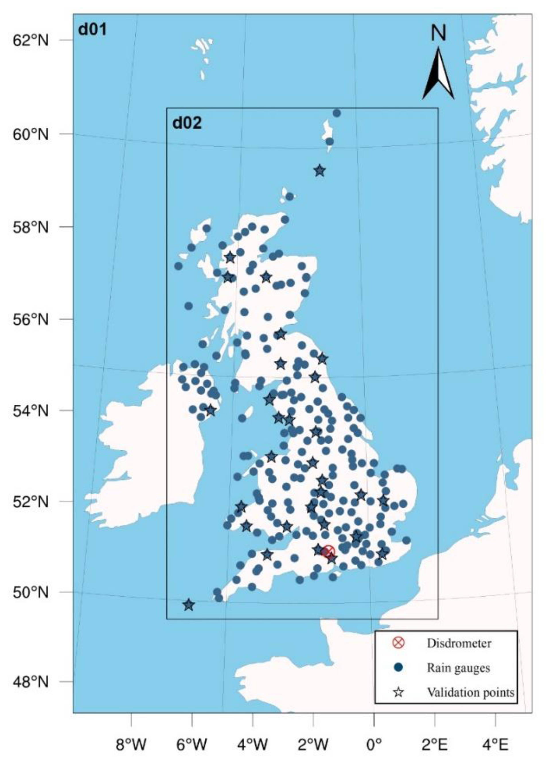
2. Study Area and Data

The study area is in the UK off the northwest coast of Europe within a range of 49°46′ N–60°43′ N and 8°25′ W–3°35′ E. This region covers approximately 248,532 km2 and comprises mainly lowland terrain with a maximum elevation of 1345 m.
The ERA-Interim datasets from the third generation of the European Centre for Medium-Range Weather Forecasts (ECMWF) reanalysis [26] were used to drive the WRF model used in the study. ERA-Interim is a significant atmospheric data source covering a data-rich period from January 1979 to the (near-real-time) present with a spatial resolution of approximately 80 km and a 3 h time interval [26]. A 2006 release of the Integrated Forecasting System (IFS-Cy31r2) was used to support the data assimilation system to produce the ERA-Interim. The system includes a four-dimensional variational analysis with a 12 h analysis window. In this study, we selected the ERA-Interim reanalysis dataset since it has been used extensively in WRF downscaling modeling studies [27,28] and performs well in rainfall simulation [29,30,31]. More details on the ERA-Interim dataset can be found on the ECMWF website at http://apps.ecmwf.int/ (accessed on 20 September 2020). For our study, five years of ERA-Interim data covering the study area from January 2013 to December 2017 were downscaled using the WRF model at temporal and spatial resolutions of 1 h and 5 km, respectively.
The tipping bucket rain gauge data were sourced from the Met Office Integrated Data Archive System Land and Marine Surface Stations data set (1853–present) [32]. These data comprise daily, hourly, and sub-hourly rain measurements, including land and marine surface observations. The bucket size was 0.2 mm, and the tip time was up to 10 s time resolution [33]. Measurements from 241 rain gauges with 1 h rainfall accumulations collected from 2013 to 2017 by the UK Met Office weather station network were selected to evaluate the accuracy of WRF rainfall simulation. Thirty rain gauges were randomly selected to validate the experimental results. The locations of the rain gauges and validation points are shown in Figure 1.
An impact-type Joss–Waldvogel (JW) disdrometer was used to analyze the appropriate interval of the shape parameter. The disdrometer was sited in southern England at 51°08′ N, 1°26′ W (Figure 1) and measured drop sizes in 127 bins from 0.3 to 5.0 mm with a sampling period and collector area of 10 s and 50 cm2, respectively. The disdrometer data provided by the British Atmospheric Data Centre cover an extended period from April 2003 to July 2018; in this study, data covering 2013 to 2017 were used to correspond with the rain gauge data. There are some uncertainties in the JW disdrometer data; for example, drops larger than approximately 5.0 mm diameter cannot be distinguished and the effect of vertical air motion on drop fall speed is neglected [34]. Therefore, raindrops larger than 5.0 mm and drizzle (rainfall intensity < 0.1 mm/h) recorded by a disdrometer were excluded from analysis in this study. In addition, to filter out the time variation previously reported [22,35,36], 10 s data measurements were averaged into 1 min periods.

3. Methodology

3.1. WRF Model Configurations

WRF model version 3.8, an Advanced Research WRF dynamical core, was used to downscale the ERA-Interim reanalysis data. The doubly nested domain configuration used in the WRF model was centered at 55°19′ N, 2°21′ W and applied at a downscaling ratio of 1:5, a finest grid of 5 km, and a temporal resolution of 1 h. In this study, we selected the 1:5 downscaling ratio rather than the 1:3 ratio, since it provides higher resolution results than the 1:3 ratio and also results in good performance of the WRF model [37]. Combining the domain center, domain size, and grid spacing, most areas in the UK can be covered as shown in Figure 1. A detailed list of the parameters used in this domain configuration is provided in Table 1. Both domains include 28 vertical pressure levels, with the top-level set at 50 hPa in each.
The simulations were performed using three different bulk double-moment microphysical parameterizations, namely, the Morrison [38], WDM6 (WRF double-moment 6-class) [15,39], and aerosol-aware Thompson [40] schemes. The Morrison scheme can predict the number concentrations of ice, snow, rain, and graupel particles; the WDM6 scheme can predict the number concentrations of cloud droplets, rain, and cloud condensation nuclei [15,39]; and the Thompson aerosol-aware scheme can predict the number concentrations of cloud droplets and ice, rain, cloud condensation nuclei, and ice nuclei [40]. For the cumulus scheme, the Kain–Fritsch scheme [41] is used, whereas the cumulus scheme is not used in the inner domain because convective rainfall generation is definitely resolved when the model grid spacing is ≤5 km [37,42]. Other physical parameterizations include the Mellor–Yamada–Janjić planetary boundary layer scheme [43], RRTM longwave radiation scheme [44], Dudhia shortwave radiation scheme [45], and Noah land-surface model [46].

3.2. Gamma RSD Model

The normalized gamma distribution is widely used to model RSD spectra because it facilitates straightforward comparisons of the microphysical characteristics of rainfall, such as raindrop diameter and number concentration [36,47], which are in the form of:
D   = N w f μ D D m μ e x p 4 + μ D D m
f μ   = 6 4 + μ μ + 4 4 4 Γ μ + 4
where N w (mm−1 mm−3), μ , and D m (mm) are the generalized intercept, shape, and mass-weighted mean diameter parameters defining the RSD spectra N D ; D is the equivalent volume diameter in mm; and Γ n is the Euler gamma function. However, a three-parameter gamma distribution [19,47,48] is used to model RSD spectra in the WRF model, which is expressed as:
N D   = N 0 D μ e λ D ,
where N 0 and λ are the intercept and slope parameters. In two-moment microphysical schemes of the WRF model, the intercept and slope parameters are obtained from the predicted number concentration N, mixing ratio q, and fixed μ as follows [38]:
N 0 = N λ μ + 1 Γ μ + 1 ,
λ = c N Γ μ + d + 1 q Γ μ + 1 1 d ,
where c and d are the coefficients of an assumed power law between mass and diameter m = c D d [38]. Based on a comparison of Equations (1) and (3), μ in the two formulas is the same, and the N 0 and λ parameters of the three-parameter gamma distribution can be converted to D m and N w parameters of normalized gamma distribution using the following equations:
D m = 4 + μ λ ,
N w = N 0 4 + μ λ μ f μ .
The RSD measured by the JW disdrometer at time instant t (s) can be obtained as follows [22,36]:
N m D i ,   t = n i t A · Δ t · V i · Δ D i ,
where m is a measured quantity, N m D i ,   t is the number of raindrops per unit volume in channel i at time t  mm 1 m 3 , n i t is the number of raindrops counted in channel i at t, A is the sensor area ( m 2 ) ,   Δ D i is the width of channel i (mm), and V i is the terminal speed of the raindrops [49] (m/s), which is expressed as:
V i = 3.78 · D i 0.67 .
The distribution of N m D i ,   t was adopted from the normalized gamma distribution fit N D [19,50,51]. μ , D m , and N w , can be estimated based on N D i . The n-order matrix m n of N D i can be calculated by:
m n = j = 1 n c D i n N D i Δ D i .
μ can be estimated as follows [52]:
μ = 7 11 γ 7 11 γ 2 4 γ 1 30 γ 12 2 γ 1 .
where γ = m 4 2 m 2 m 6 . D m is calculated by:
D m = m 4 m 3 ,
and N w can be estimated from:
N w = 256 6 m 3 5 m 4 4 .
The rainfall intensity (mm/h) R in each rainfall step of the WRF or JW disdrometer is obtained from the RSD as:
R = 6 π · 10 4 0 D 3 V D N D d D .

3.3. Experimental Designs

We determined whether a gamma RSD model with an adaptive shape parameter of WRF double-moment microphysical parameterization could improve the accuracy of WRF rainfall retrieval. An adaptive-μ model of the gamma distribution based on rainfall intensity was tested over six scenarios comprising three double-moment schemes and two seasons. To focus on liquid precipitation analyses, hail and snow were excluded from this study according to temperature, drop size, and ground weather reports.
Figure 2 presents the experimental flowchart of this study. As an initial step, five years of ERA-Interim data were downscaled by applying the WRF model under different double-moment schemes, i.e., Morrison, WDM6, and Thompson aerosol-aware MPs, to obtain long-term WRF simulation results. To simulate the continuous WRF results for each year, we ran the model monthly with a spin-up time of 12 h [53] for the three MPs using the configurations described in Section 3.1. This study only used the lowest-level and inner-domain of the WRF results. The RSDs of different double-moment schemes were calculated based on the predicted number concentration and mixing ratio variables of the WRF outputs using Equations (4) and (5).
Second, we analyzed the characteristics of the WRF RSD simulation results of three schemes. The D m l o g 10 N w relationship and D m R relationship of the three schemes in the WRF model were investigated by comparison of these relationships with the JW disdrometer in this study. The rainfall characteristics of different seasons are very different, which is worth studying. Concerning the climatic seasonal characteristics of the UK, we separated the four seasons into cold (23 September–19 March) and warm seasons (20 March–22 September) [22]. Based on the five years of disdrometer-observed RSD, the constraint interval of the shape parameter for different seasons was calculated.
Third, we used the three-parameter RSD model by applying the adaptive-μ method to improve the performance of WRF rainfall simulation. We modified the shape parameter μ in the RSD model to introduce one extra degree of freedom to it to improve its fitness. We searched for the optimal μ within the constraint interval of rainfall intensities following the principle of minimizing the WRF rainfall simulation error by comparing observed rainfall data for different seasons with results produced by three double-moment microphysics schemes. According to the three-parameter gamma RSD model and Equations (4) and (5), the N 0 and λ parameters are computed based on the shape parameter μ; thus, the N 0 and λ parameters will also be changed by μ. The root-mean-square error (RMSE) in mm was selected as the objective function of the optimization algorithm, as shown in Equation (15), and can range from zero to infinity, with a lower value corresponding to a better fit to the observed data:
RMSE = 1 N i = 1 N R i G i 2 ,
where G i and R i are the rainfall intensity of each rainfall step at time i derived from the rain gauge rainfall data and the corresponding location of the WRF RSD data, respectively, and N is the total number of rainfall steps. The genetic algorithm (GA), which is inspired by natural selection processes involved in biological evolution [54], can solve both constrained and unconstrained optimization problems and can avoid being trapped at locally optimal solutions [55]. The main characteristics of GA include coding of the parameter set rather than the parameters themselves, initiating its search from multiple points rather than a single point, applying payoff information rather than derivatives, and using probabilistic transition rules rather than deterministic ones [56]. There are three main genetic operators of GA, namely, reproduction, crossover, and mutation [56]. The optimization search procedure in GA is based on the principle of natural selection and natural genetics. We implemented GA optimization to minimize the value of the RMSE when searching for the optimal μ at different rainfall intensities. Depending on the relationship between the optimal μ and rainfall intensity, a linear adaptive-μ model was proposed for each combination of the season and double-moment scheme.
Finally, we applied the adaptive-μ models to the 30 validation points to test their reliability and applicability relative to a fixed-μ model. As the adaptive-μ models were established to improve the precision of WRF rainfall simulation, two other commonly used model performance evaluation indices, mean bias error (MBE) and standard deviation (SD) (Equations (16) and (17), respectively), were used in addition to RMSE to validate the model [37,57]:
MBE = 1 N i = 1 N R i G i ,
SD = 1 N 1 j = 1 N R i G i MBE 2 ,
A perfect MBE score of 0 indicates a low overall magnitude of bias in the simulated data, which is essential in hydrological applications. The SD can be used to measure random error; a low value indicates a slight variation from the MBE.

4. Results

4.1. WRF RSD Simulation Results of Different Double-Moment MPs

To build a model that produces an optimal gamma distribution shape parameter reflecting changes in rainfall intensity by season, we ran the WRF model under different double-moment schemes using long-term ERA-Interim data. The three-dimensional values of N 0 and λ parameters in the gamma RSD model were calculated from the N and q variables of the lowest level in the WRF simulation outputs based on Equations (4) and (5). Using Equations (6) and (7), the values of D m and N w were then calculated. Figure 3 shows the map of the average values of D m and l o g 10 N w and the annual rainfall from 2013 to 2017 under the Morrison scheme. This figure indicates that the spatial distribution trend of the average D m and l o g 10 N w as well as that of annual rainfall in different years was consistent, although the number varied by year. The value of average D m presented a trend of gradual increase from north to south and west to east, whereas the values of l o g 10 N w and annual rainfall showed a trend of gradual decrease from north to south and from west to east. These trends indicate that rainfall information can be reflected through the values of the RSD parameters in the WRF model, such that a smaller average value of D m or larger average value of l o g 10 N w indicates higher annual rainfall. The annual average value of RSD and annual rainfall results of WDM6 and Thompson aerosol-aware schemes displayed similar patterns; therefore, the analysis does not present these schemes separately.
The D m and N w in the observation were calculated from the raindrop data recorded by the JW disdrometer. To accurately compare the observed and simulated D m and N w , we extracted the grid (coordinates are 51°08′ N and 1°26′ W with a grid size of 5 km × 5 km) in the WRF simulation that was closest to the JW disdrometer with the same time span. Figure 4 shows the occurrences of the relationship between D m and l o g 10 N w of the Morrison, WDM6, and Thompson aerosol-aware schemes, and the JW disdrometer. The D m l o g 10 N w density scatter plots show a fan shape centered at the D m between approximately 0.5 mm and 1.5 mm. The D m l o g 10 N w relation showed a negative correlation, which can be fitted by a quadratic polynomial function in the form of l o g 10 N w  = a D m 2 + b D m + c [58]. The fitting curves between D m and l o g 10 N w and corresponding R-squared (R2) statistic of different schemes and the JW disdrometer are also presented in Figure 4. R2 is a metric that measures the degree of dependence between variables in a regression model with a range of 0 to 1, where a higher value of R2 generally reflects a better fit between the model and data. Compared to the fitting curve of the JW disdrometer, the fitting coefficients of the WRF model were quite close to those of the JW disdrometer, with the values of R2 larger than 0.70. Among the three schemes, the fitting curve of Morrison showed the highest degree of similarity with that of the JW disdrometer. These results demonstrate that the WRF model can identify relationships between D m and l o g 10 N w , whereas there are some uncertainties between different schemes.
Figure 5 shows the occurrences of the relationship between R and D m of the Morrison, WDM6, and Thompson aerosol-aware schemes, and the JW disdrometer. R and D m showed a positive correlation, that is, the size of raindrops increased gradually with increasing rainfall intensity. The R - D m relationship can be fitted by a power-law function in the form of D m = a R b [59,60]. The fitting curves between R and D m and the corresponding R2 of different schemes and the JW disdrometer are also presented in Figure 5. All double-moment schemes identified a power-law relationship between R and D m , whereas the values of fitting coefficients and R2 of different schemes showed a certain gap. Among the three schemes, the fitting curve of the Morrison scheme was closest to that of the JW disdrometer, whereas the R2 value of the Thompson aerosol-aware scheme was relatively small.

4.2. Shape Parameter Constraint Interval

Figure 6 shows the reasonable ranges of the gamma RSD model shape parameter for warm and cold seasons, respectively, based on the five years of disdrometer data. Given these wide ranges, the middle 95% values were adopted as constraint intervals (gray-highlighted regions in the figure) to improve the efficiency of the optimization algorithm. The warm season had a wider constraint interval, ranging from 0 to 48, than the cold season, which ranged from 0 to 39.

4.3. Empirical Formula of Adaptive Shape Parameter in the WRF RSD Model

We modified the shape parameter μ in the RSD model to bring one extra degree of freedom to it to improve its fitness. The shape parameter μ is computed based on the μ–R relationship by adopting the GA method to search for the optimal μ for different seasons and microphysical schemes. The search goal of GA is to minimize the value of RMSE between the observed and WRF-simulated rainfall. There are five phases in the GA search procedure, including initial population, fitness function, selection, crossover, and mutation. Since extreme rainfall data were insufficient within the study area, the optimal μ value under a rainfall intensity >9.5 mm/h will not be representative and can lead to uncertainty for the adaptive-μ model. Therefore, only rainfall with intensities of ≤9.5 mm/h was considered in this study. Figure 7 shows the 211 rain gauges observed and the corresponding WRF-simulated rainfalls produced at fixed and optimal values of μ for the two seasons and three double-moment schemes. For all three schemes, adopting the optimal μ resulted in a distinct decrease in RMSE relative to the fixed-μ case, although in each case, this difference was difficult to distinguish when the rainfall intensity was <1.5 mm/h, indicating that at rainfall intensities <1.5 mm/h, the adaptive-μ model cannot improve the performance of WRF rainfall simulation. Therefore, the fixed-μ gamma RSD model is suitable for double-moment microphysics in this low-rainfall-intensity regime. In other words, μ equaled 0 for the Morrison and Thompson aerosol-aware schemes and μ equaled 1 for the WDM6 scheme when rainfall intensities were <1.5 mm/h. We restricted our further investigation of the relationship between optimal μ and rainfall intensity to intensities > 1.5 mm/h.
Figure 8 shows the optimal μ of rainfall intensity by scenarios. The optimal value of μ tended to increase as rainfall intensity increased, with a clear linear relationship between optimal μ and rainfall intensity for all three schemes. We applied the ordinary least-squares regression method to select a linear function to relate the rainfall intensity and optimal μ data points at intensities ≥1.5 mm/h. The R2 statistic for each scheme is also shown in Figure 8. Overall, the R2 values between rainfall intensity and optimal μ indicate that the selected linear functions represented reasonable models for fitting the data. Notably, the values were higher in the cold season than in the warm season for all three double-moment schemes, suggesting that the linear relationship between rainfall intensity and optimal μ is more prominent during cold seasons.
Despite good fit, there remain differences among the respective linear empirical formulas. The constant term of the empirical Morrison scheme formula was higher than that in the Thompson aerosol-aware scheme, which was higher than that in the WDM6 scheme. In contrast, the independent variable coefficient under the Thompson scheme was lower than in the others.
The differing results by seasons suggest that the respective adaptive-μ models of the gamma RSD distribution under WRF double-moment bulk schemes based on rainfall intensity (mm/h) can be expressed as piecewise functions (equations listed in Table 2). In addition, as this study excluded rainfall data with R > 9.5 mm/h, we could not confirm whether the adaptive-μ model proposed in this study is suitable for extreme rainfall over the study area. This study suggests that the fixed-μ gamma RSD model can be adopted, i.e., it is not necessary to adjust the value of WRF-simulated R for extreme rainfall.

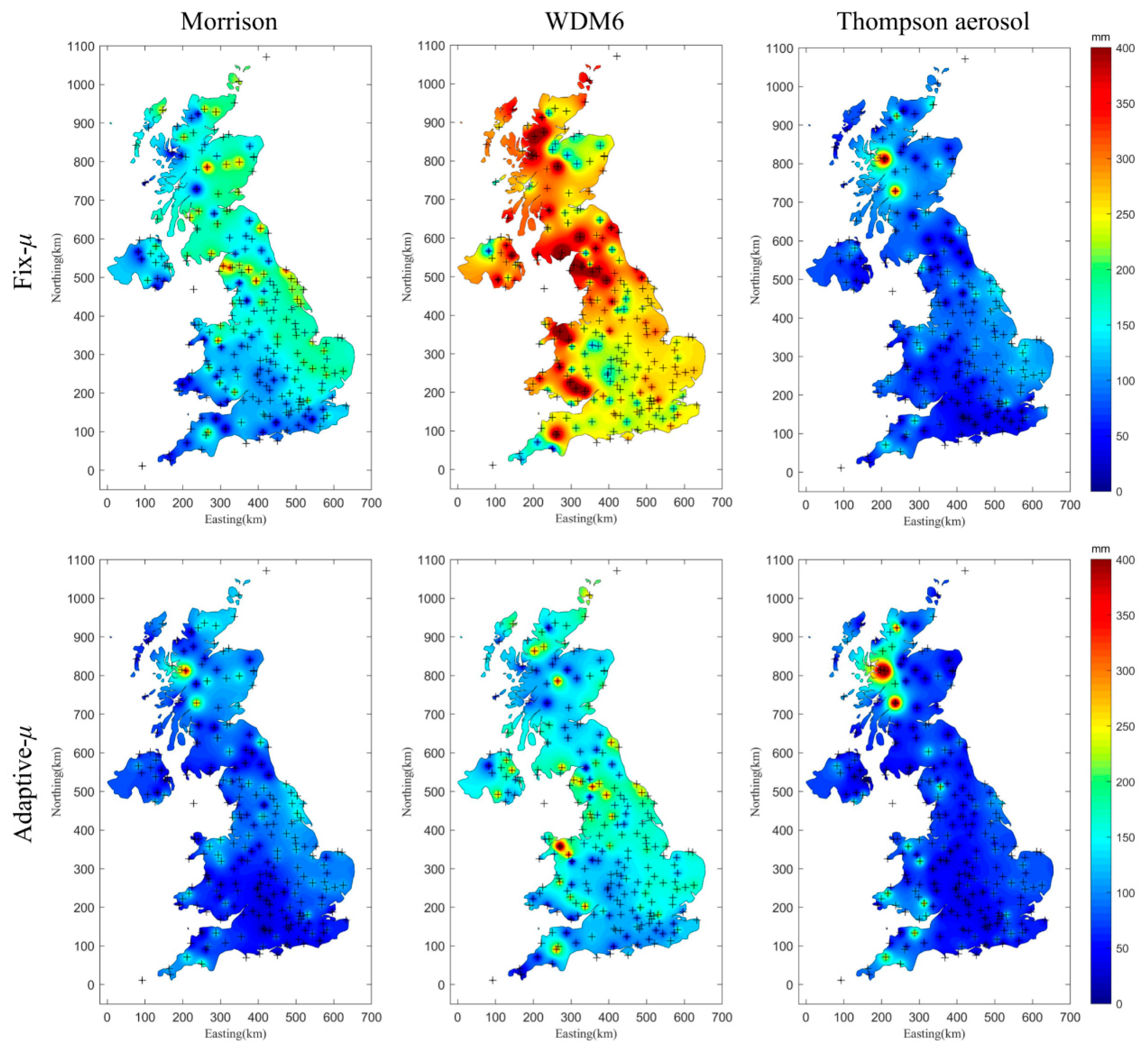
4.4. WRF Rainfall Results of Different Scenarios

We computed the WRF rainfall using the adaptive-μ models of the gamma RSD distribution. Using the rain gauge rainfall as a benchmark, we calculated the WRF and rain gauge rainfall difference using the fixed- μ and adaptive- μ RSD models. Figure 9 and Figure 10 show the spatial distribution of the absolute value of the annual rainfall amount difference between the WRF simulation and rain gauge of different scenarios in 2013 and 2016 (the results in 2014, 2015, and 2017 are shown in the Figures S1–S3). Values other than the position of the rain gauge were interpolated via the kriging method [61,62]. Kriging is an interpolation method stemming from regionalized variable theory for geographical information systems [61]. Due to the nature of the spatial interpolation process, the extreme values are typically associated with the rain gauge locations. From these two figures, among three schemes, the annual rainfall simulated by the Thompson aerosol-aware scheme was closest to the actual value, whereas the WDM6 results were the least concordant. Compared with the annual rainfall difference of the fixed- μ RSD model, the map’s color had a larger area of blue for the adaptive-μ RSD model, particularly for the WDM6 model. This illustrates that for most sites, the annual rainfall differences in the adaptive-μ RSD model were smaller than those of the fixed- μ RSD model for different double-moment schemes. From the perspective of the spatial distribution of the annual rainfall difference, the adaptive-μ RSD models of Morrison and Thompson aerosol-aware schemes showed good performance in the eastern and southern regions of the UK, whereas some sites exhibited relatively poor performance in the northern region of the UK.

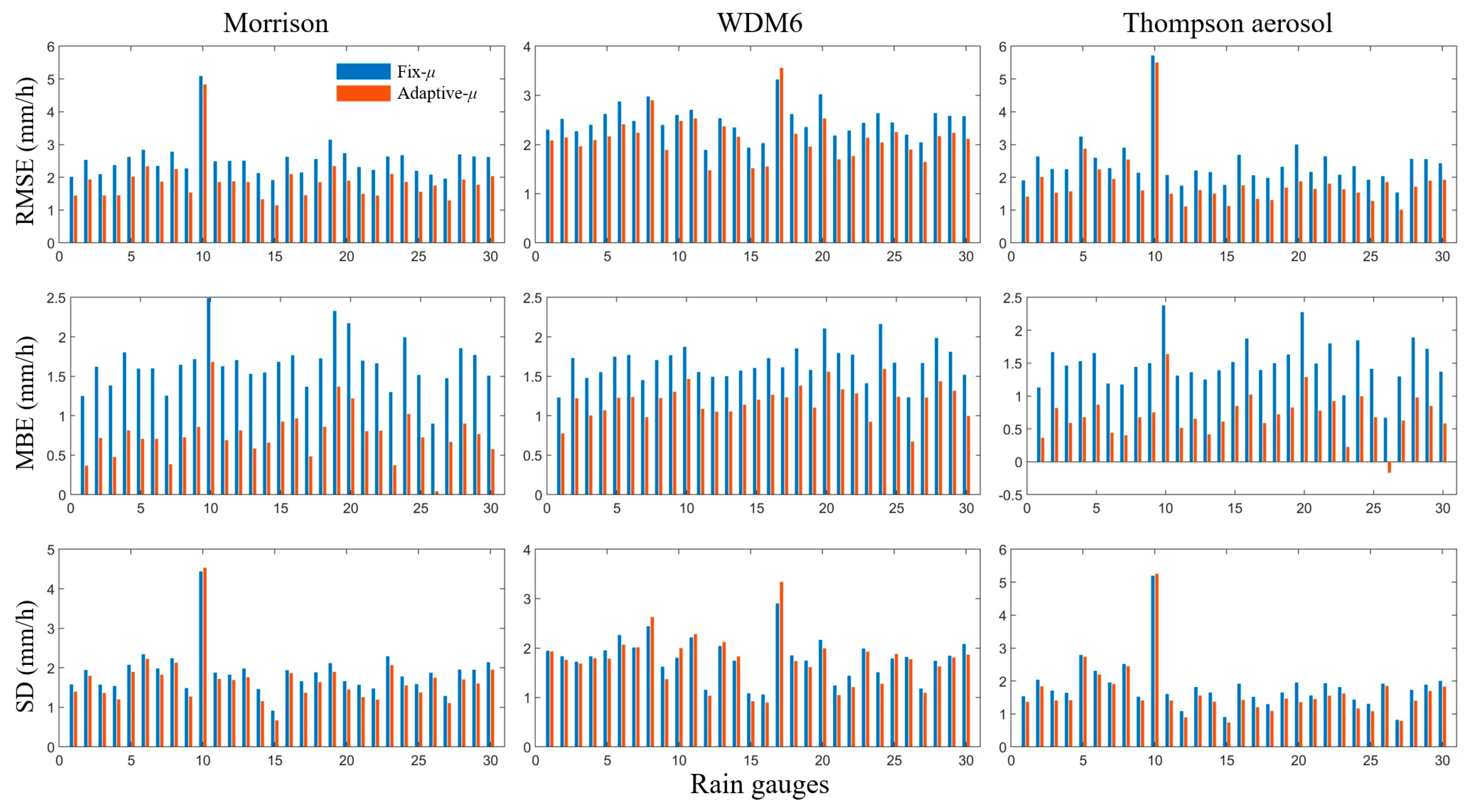
4.5. Validation of the Adaptive-μ Model

Five years of WRF simulation and rain gauge data from 30 validation points were used to examine the applicability of the adaptive-μ model proposed in Section 3.2 to the study region. The RMSE, MBE, and SD error indices were used to investigate whether the adaptive-μ model for the WRF double-moment microphysics schemes could enhance the accuracy of WRF rainfall retrieval and to quantify any improvements obtained. Figure 11 shows the results of the fixed- and adaptive-μ indices at rainfall intensities higher than 1.5 mm/h for 30 validation points and different schemes. Compared with the results obtained using the fixed-μ model, all validation points of the Morrison and Thompson aerosol-aware schemes and 29 validation points of the WDM6 showed smaller RMSE values, and all rain gauges of the three schemes showed smaller MBE values. In contrast, only one point of the Morrison and Thompson aerosol-aware schemes and seven rain gauges of the WDM6 had larger SD values using the adaptive-μ model. These results demonstrate that the adaptive-μ model had better performance than the fix-μ model in almost all validation sites.
Table 3, Table 4 and Table 5 list the values of the fixed- and adaptive-μ indices at rainfall intensities higher than 1.5 mm/h for each of the three models along with the improvements (IMPROV% columns) obtained using adaptive-μ parameters as measured using each index. For each combination of the warm and cold seasons and application of the Morrison, WDM6, and Thompson aerosol-aware double-moment schemes, the RMSEs were decreased by 18.46%, 28.77%, 7.27%, 15.38%, 18.18%, and 26.24%, respectively. Similarly, the MBEs were decreased by 54.12%, 65.67%, 27.68%, 34.51%, 50.88%, and 58.27% for the respective combinations. Finally, the SDs were improved by 7.17%, 20.61%, 0.98%, 7.30%, 7.66%, and 19.15% under the respective season and scheme combinations.
These validation results demonstrate that the linear adaptive-μ model can more accurately capture rainfall intensity than the fixed-μ model. Applying the adaptive-μ model during the cold season results in a more remarkable improvement in the accuracy of the WRF rainfall simulation results than is achieved by applying this model during the warm season. The relatively low level of improvement obtained for the WDM6 scheme suggests that the sensitivity to the adaptive-μ model sensitivity differed for each scheme.

5. Discussion

This study was conducted based on the assumption that double-moment bulk microphysical parameterizations of the WRF model using a fixed value of the gamma RSD model shape parameter can be improved. To improve WRF rainfall retrieval, we used an adaptive-μ model to study the rainfall records covering most of the UK landmass over five years (2013 to 2017). Under the assumption that the μ-value might vary by rainfall intensity, the GA method was used to search for optimal values of μ by rainfall intensity during different seasons and under varying double-moment bulk microphysics. Empirical formulas relating rainfall intensity to optimal μ were then built using the ordinary least-squares linear regression method and, based on these, adaptive-μ models of the gamma distribution were proposed for the respective scenarios. Our experimental results were used to address the three following primary issues.
The first issue related to whether using an adaptive value of the shape parameter of the gamma RSD model could improve the performance of WRF rainfall simulation. The results revealed a significant decline in the RMSE using the optimal μ of different rainfall intensities rather than the constant value of μ in the gamma RSD model, particularly for high rainfall intensity. However, the optimal μ of low rainfall intensity (R < 1.5 mm/h) did not clearly reduce the WRF-simulated rainfall error, indicating that the fixed-μ gamma RSD model is suitable when rainfall intensity is low (<1.5 mm/h) for the studied microphysics schemes. Given that the calculation efficiency could be reduced using the adaptive-μ model and the performance of WRF rainfall retrieval could not be improved, for low rainfall intensity, there is no need to determine the relationship between rainfall intensity and the optimal μ, and fixing the value of the shape parameter to 0 or 1 of the gamma RSD model is feasible for WRF double-moment microphysics schemes.
The second issue was whether a suitable model can accurately describe the relationship between rainfall intensity and the optimal μ under multiple scenarios. Our results demonstrate that, at rainfall intensities of ≥1.5 mm/h, a linear function can fit rainfall intensity to the optimal μ exceedingly well for different seasons and under various double-moment schemes. However, although there was a robust linear relationship between rainfall intensity and the optimized μ, the empirical formulas differed by scenario, suggesting that no unified adaptive-μ parameter formulation fits all scenarios (i.e., different seasons and microphysics schemes) over the specific study area. The empirical formulas for the Morrison scheme were relatively similar by seasons, whereas those for the other two schemes differed significantly. Thus, the adaptive-μ empirical formulas proposed in this study are universally applicable to the microphysics schemes and regions studied.
The third issue was validating the empirical formulas and examining how well the adaptive-μ model could improve WRF-simulated rainfall accuracy. Our validation results indicate that the adaptive-μ gamma RSD model outperformed a fixed-μ WRF double-moment microphysics model in terms of at least three error indices. The results also indicate that the improvements in WRF rainfall retrieval obtained by applying the adaptive-μ gamma RSD model differed by scenario.
The proposed model performed better during cold seasons and the various double-moment schemes assessed had distinct sensitivities to the model, which are reflected in the fact that the R2 values of the fitted lines produced by the adaptive-μ model were higher in the warm season than in the cold season. These results may also relate to differences in the probability distribution of rainfall intensity between seasons. As shown in Figure 12, in the region studied, the cold season had a higher probability density for low rainfall intensity (i.e., R < 2.8 mm/h) and a lower probability density for high rainfall intensity than the warm season. This differentiation by season may enhance the WRF rainfall simulation accuracy during the cold season when applying the adaptive-μ model.
The RMSEs obtained under the Morrison and Thompson aerosol-aware schemes were decreased by more than 15% and 25%, respectively, during the cold season, whereas the respective MBEs were decreased by more than 50% and 55%, and the SDs were decreased by approximately 7% and close to 20%, respectively. The degree of error reduction under the WDM6 scheme, however, was much lower. The significant reduction in the error of WRF rainfall retrieval under the former two schemes using the adaptive-μ model suggests that the adaptive-μ model can successfully be combined with these schemes.
Because the data from 241 rain gauges used to validate the WRF rainfall simulations produced limited information on rainfall microphysics and RSD, the adaptive-μ gamma RSD models assessed in this study could only be examined through statistical error analysis. In contrast, the physical mechanisms underlying the model could not be explored. Two important data sources for validating numerically simulated WRF precipitation microphysics—disdrometer observations and dual-polarization radar reflectivity data—could be applied to the mechanistic modification of the gamma RSD model of WRF double-moment microphysics. As disdrometer samplings were already imitated within the study area, in future studies, dual-polarization radar data will be used to further examine the adaptive-μ gamma RSD model in terms of additional variables (e.g., median drop diameter D0, differential reflectivity ZDR, and specific differential phase KDP) related to the microphysics of RSD.

6. Conclusions

To construct a model that would produce an optimal gamma distribution shape parameter reflecting changes in rainfall intensity by season, five years of ERA-Interim data were downscaled by applying the WRF model under different double-moment schemes; the results were compared with observations taken at 241 rain gauges and one disdrometer during the same period. We concluded the following from the analysis results.
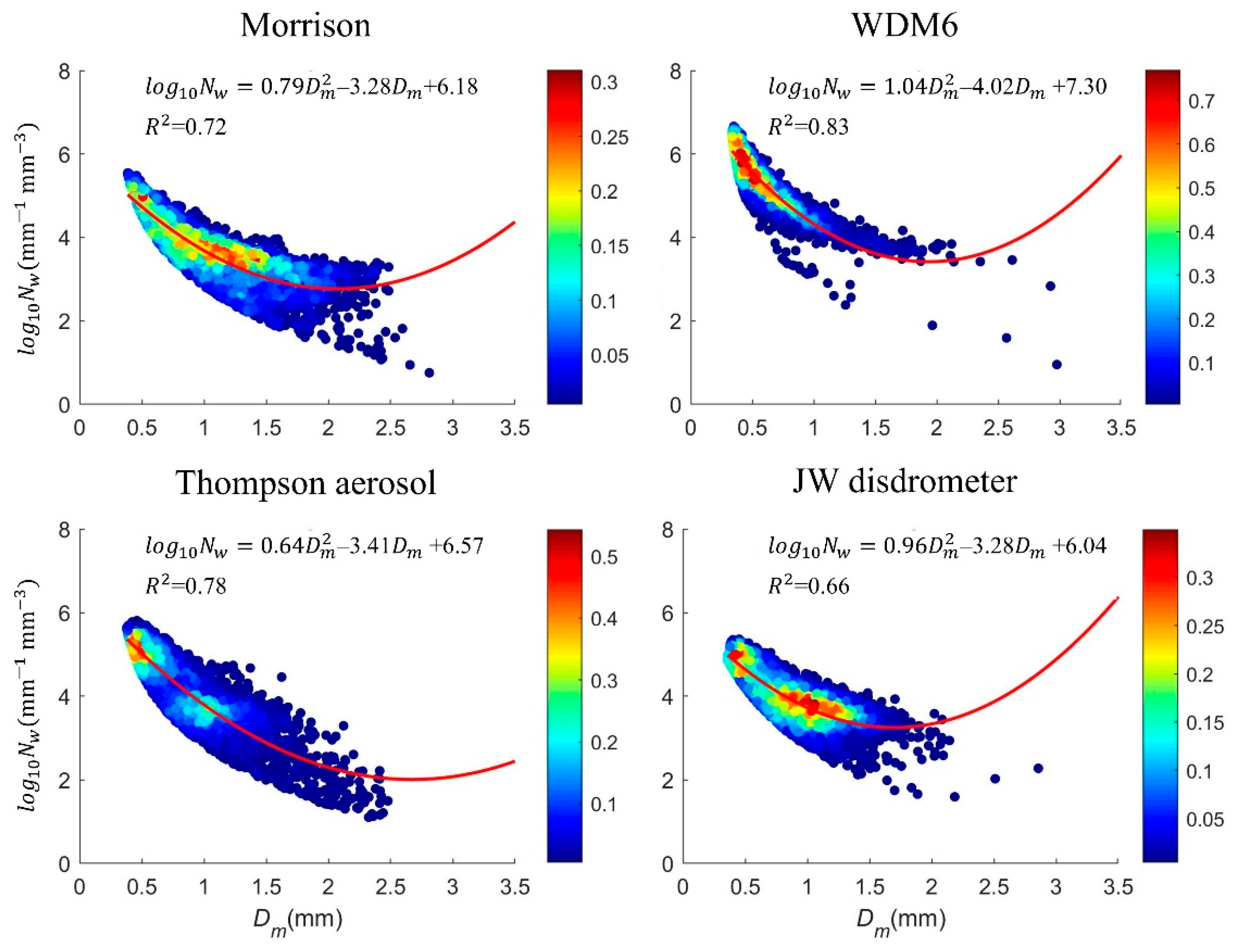
  • The spatial characteristics of rainfall can be reflected by the WRF-simulated RSD, with a smaller average value of D m or larger average value of l o g 10 N w , associated with higher annual rainfall. Similar to the RSD results of the JW disdrometer, the three tested WRF double-moment schemes showed a strong quadratic relationship between D m and l o g 10 N w and a clear power-law relationship between R and D m , although there were some uncertainties between different schemes.
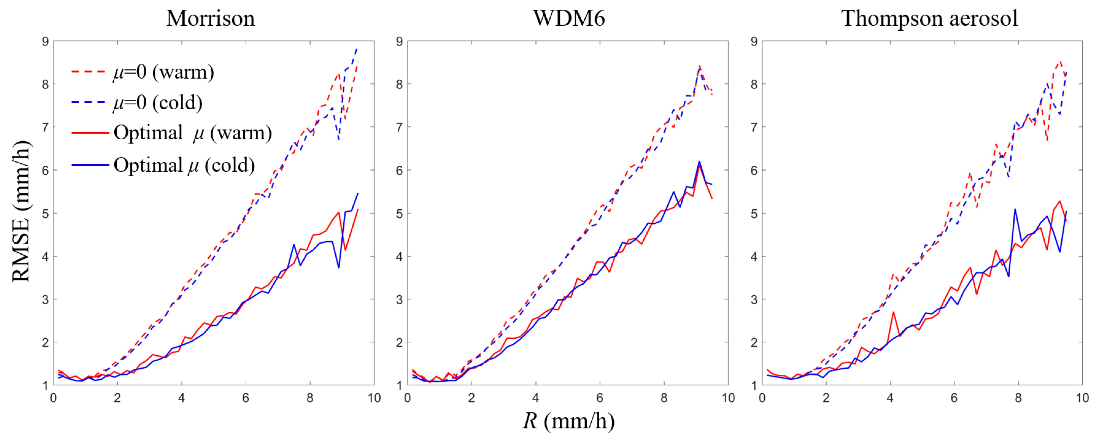
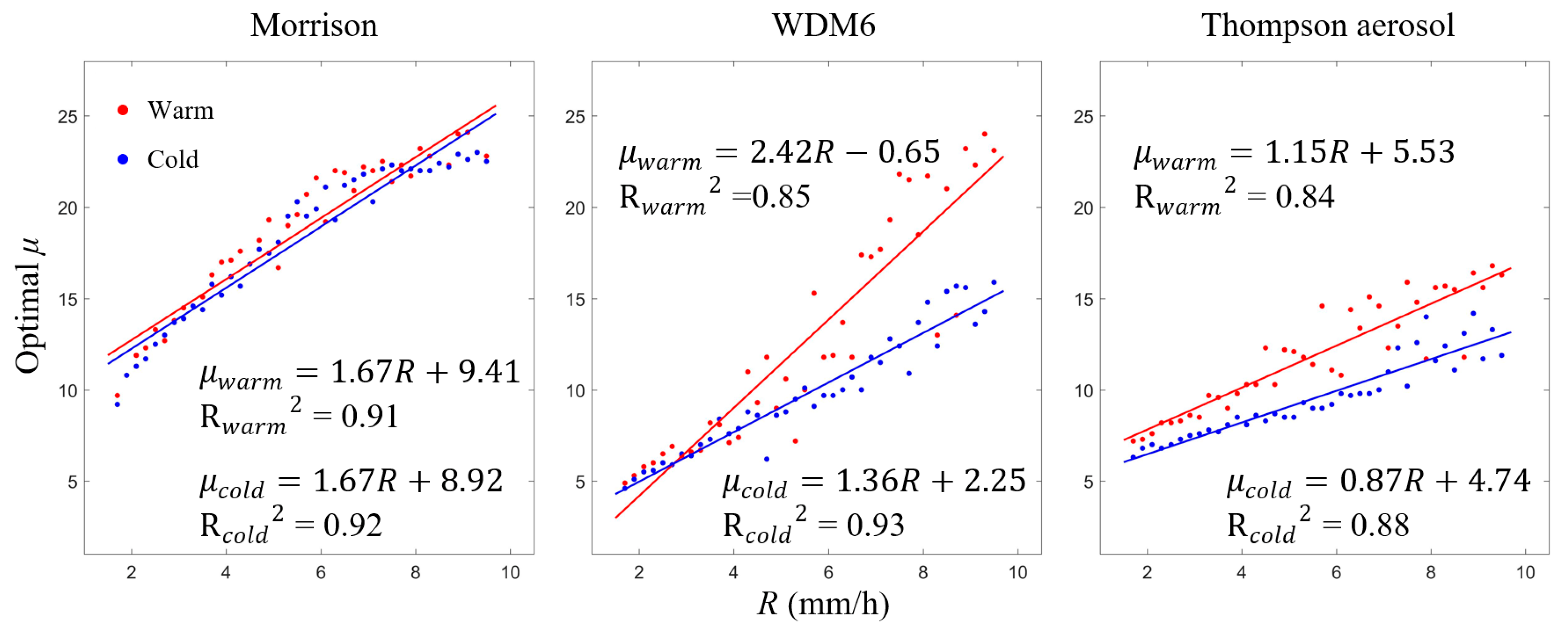
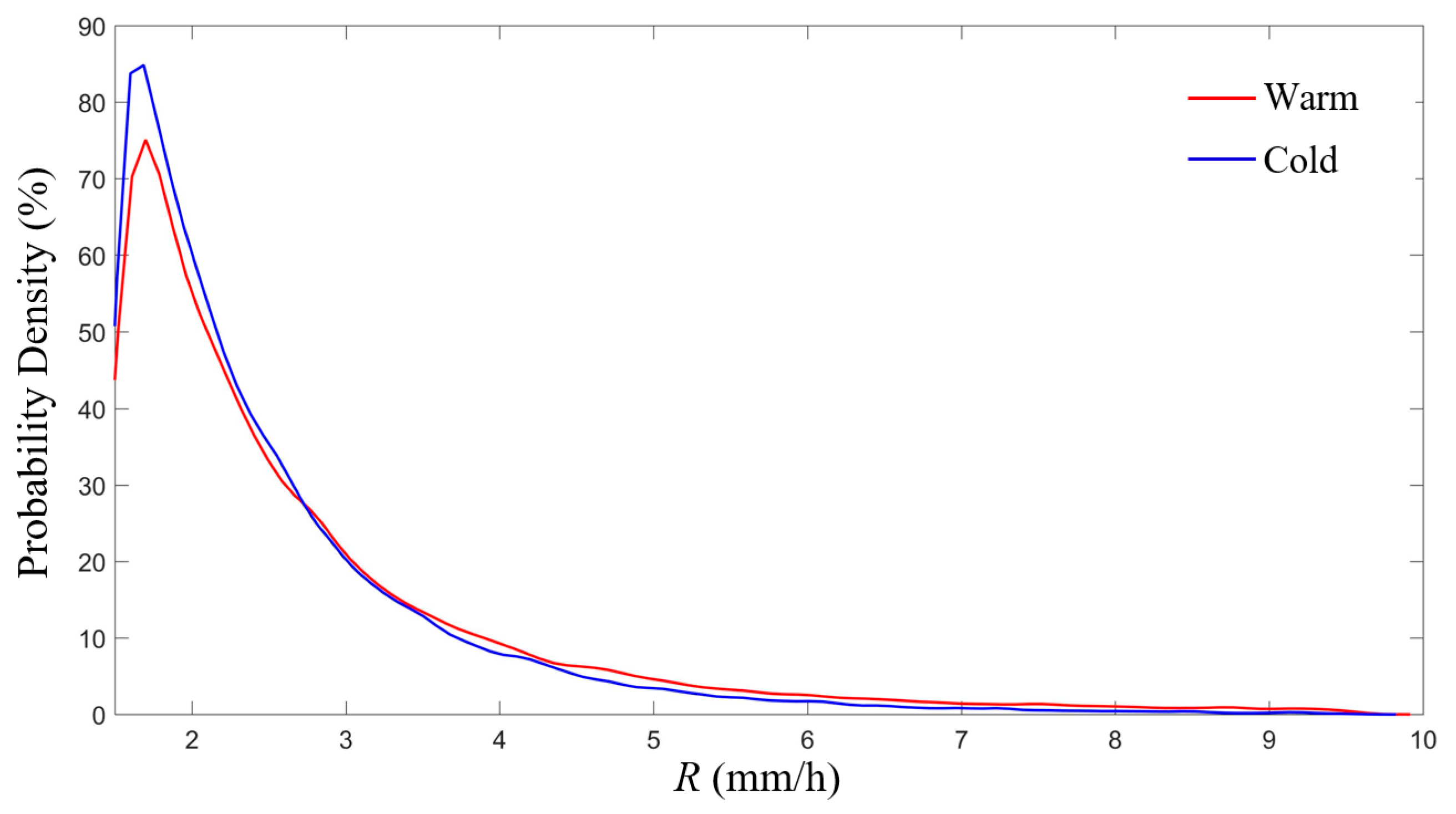
  • Although the fixed-μ gamma RSD model was suitable when rainfall intensity was <1.5 mm/h, linear empirical formulas relating rainfall intensity to optimal μ were successfully built to reflect different scenarios for which the rainfall intensity was ≥1.5 mm/h. Adaptive-μ models of the gamma distribution based on rainfall can be constructed using a piecewise function, as shown in the following equation:
    μ = c o n s t a n t ,               R < 1.5 a R + b ,     1.5 R 9.5 ,
    where R is the rainfall intensity in mm/h, a is the coefficient of the independent variable, and b is the constant term of the linear function. Adaptive-μ models of the gamma distribution were constructed to apply the Morrison, WDM6, and Thompson aerosol-aware double-moment schemes to two seasons (Table 2).
  • The consistency and usability of the adaptive-μ model were also demonstrated by using three error indices by applying the model to 30 validation points. A higher degree of error reduction was observed during the cold season, whereas the Morrison and Thompson aerosol-aware schemes achieved higher degrees of error reduction overall compared to the WDM6 scheme. The adaptive-μ model showed improved predictability for the three tested double-moment schemes compared to the fixed-μ model, indicated by the decreases in RMSE by 23.62%, 11.33%, and 22.21%; decreases in MBE by 59.90%, 31.10%, and 54.58%; and decreases in SD by 13.89%, 4.14%, and 13.41% for the Morrison, WDM6, and Thompson aerosol-aware schemes, respectively.
Based on the above results, the adaptive-μ model of gamma distribution can be successfully integrated into WRF double-moment microphysics scheme simulations to improve the accuracy of WRF rainfall retrieval, particularly during cold seasons and when using the Morrison and Thompson aerosol-aware schemes. This method and the relevant optimal μ-values are appropriate for the study area in the UK and can potentially be incorporated into the WRF model as part of its simulation process. The adaptive-μ model was designed to reduce simulated rainfall error in the WRF model by applying the observed rain gauge data. As we could not explore the physical mechanisms underpinning the adaptive-μ results in this study, further application of additional data sources (e.g., dual-polarization radar data) should be performed to study the RSD model in WRF bulk microphysics schemes based on additional variables related to precipitation microphysics.

Supplementary Materials

The following supporting information can be downloaded at: https://www.mdpi.com/article/10.3390/atmos13010036/s1. Figure S1. The absolute value of the annual rainfall amount difference between the WRF simulation and rain gauge using fixed-μ and adaptive-μ RSD models of three double-moment schemes in 2014. Figure S2. The absolute value of the annual rainfall amount difference between the WRF simulation and rain gauge using fixed-μ and adaptive-μ RSD models of three double-moment schemes in 2015. Figure S3. The absolute value of the annual rainfall amount difference between the WRF simulation and rain gauge using fixed-μ and adaptive-μ RSD models of three double-moment schemes in 2017.

Author Contributions

Conceptualization, S.Z. and Q.D.; methodology, Q.Y. and S.Z.; software, Q.Y.; validation, Q.Y. and H.Z.; formal analysis, Q.D.; investigation, Q.Y.; resources, Q.Y.; data curation, H.Z.; writing—original draft preparation, Q.Y.; writing—review and editing, S.Z.; visualization, Q.D.; supervision, S.Z.; project administration, S.Z. and Q.Y.; funding acquisition, S.Z. All authors have read and agreed to the published version of the manuscript.

Funding

This research was funded by the National Natural Science Foundation of China (Nos: 42071364, 42101416, and 41871299) and the China Postdoctoral Science Foundation Funded Project (No. 2021M691628).

Institutional Review Board Statement

Not applicable.

Informed Consent Statement

Not applicable.

Data Availability Statement

Not applicable.

Acknowledgments

We thank the Advanced Computing Research Centre at the University of Bristol for providing the access to the high-performance computing (HPC) system BlueCrystal. The ERA-Interim data driving the WRF model can be downloaded from the ECMWF Public Datasets web interface (https://www.ecmwf.int/ (accessed on 18 May 2021)). The gauge data sets and disdrometer were sourced from the UK Met Office and British Atmospheric Data Centre at http://archive.ceda.ac.uk/ (accessed on 18 May 2021).

Conflicts of Interest

The authors declare no conflict of interest.

References

  1. Cao, Q.; Zhang, G. Errors in Estimating Raindrop Size Distribution Parameters Employing Disdrometer and Simulated Raindrop Spectra. J. Appl. Meteorol. Climatol. 2009, 48, 406–425. [Google Scholar] [CrossRef]
  2. Yang, Q.; Dai, Q.; Han, D.; Chen, Y.; Zhang, S. Sensitivity analysis of raindrop size distribution parameterizations in WRF rainfall simulation. Atmos. Res. 2019, 228, 1–13. [Google Scholar] [CrossRef]
  3. Ma, Y.; Ni, G.; Chandra, C.V.; Tian, F.; Chen, H. Statistical characteristics of raindrop size distribution during rainy seasons in Beijing urban area and implications for radar rainfall estimation. Hydrol. Earth Syst. Sci. 2019, 23, 4153–4170. [Google Scholar] [CrossRef] [Green Version]
  4. Zhu, J.; Zhang, S.; Yang, Q.; Shen, Q.; Zhuo, L.; Dai, Q. Comparison of rainfall microphysics characteristics derived by numerical weather prediction modelling and dual-frequency precipitation radar. Meteorol. Appl. 2021, 28, e2000. [Google Scholar] [CrossRef]
  5. Caracciolo, C.; Napoli, M.; Porcù, F.; Prodi, F.; Dietrich, S.; Zanchi, C.; Orlandini, S. Raindrop size distribution and soil erosion. J. Irrig. Drain. Eng. 2012, 138, 461–469. [Google Scholar] [CrossRef]
  6. Janapati, J.; Seela, B.K.; Lin, P.-L.; Wang, P.K.; Kumar, U. An assessment of tropical cyclones rainfall erosivity for Taiwan. Sci. Rep. 2019, 9, 1–14. [Google Scholar]
  7. Michaelides, S.; Levizzani, V.; Anagnostou, E.; Bauer, P.; Kasparis, T.; Lane, J.E. Precipitation: Measurement, remote sensing, climatology and modeling. Atmos. Res. 2009, 94, 512–533. [Google Scholar] [CrossRef]
  8. Dai, Q.; Zhu, J.; Zhang, S.; Zhu, S.; Han, D.; Lv, G. Estimation of rainfall erosivity based on WRF-derived raindrop size distributions. Hydrol. Earth Syst. Sci. 2020, 24, 5407–5422. [Google Scholar] [CrossRef]
  9. Skamarock, W.C.; Klemp, J.B.; Dudhia, J.; Gill, D.O.; Barker, D.M.; Wang, W.; Powers, J.G. A Description of the Advanced Research WRF Version 2. National Center for Atmospheric Research Boulder Co Mesoscale and Microscale Meteorology Div 2005. Available online: https://apps.dtic.mil/sti/citations/ADA487419 (accessed on 25 December 2021).
  10. Skamarock, W.C.; Klemp, J.B.; Dudhia, J.; Gill, D.O.; Barker, D.M.; Wang, W.; Powers, J.G. A Description of the Advanced Research WRF Version 3. NCAR Technical Note-475+STR 2008. Available online: http://citeseerx.ist.psu.edu/viewdoc/summary?doi=10.1.1.484.3656 (accessed on 25 December 2021).
  11. Dai, Q.; Han, D. Exploration of discrepancy between radar and gauge rainfall estimates driven by wind fields. Water Resour. Res. 2014, 50, 8571–8588. [Google Scholar] [CrossRef]
  12. Crétat, J.; Pohl, B.; Richard, Y.; Drobinski, P. Uncertainties in simulating regional climate of Southern Africa: Sensitivity to physical parameterizations using WRF. Clim. Dyn. 2012, 38, 613–634. [Google Scholar] [CrossRef]
  13. Dawson, D.T.; Xue, M.; Milbrandt, J.A.; Yau, M. Comparison of evaporation and cold pool development between single-moment and multimoment bulk microphysics schemes in idealized simulations of tornadic thunderstorms. Mon. Weather. Rev. 2010, 138, 1152–1171. [Google Scholar] [CrossRef]
  14. Johnson, M.; Jung, Y.; Dawson, D.T.; Xue, M. Comparison of simulated polarimetric signatures in idealized supercell storms using two-moment bulk microphysics schemes in WRF. Mon. Weather. Rev. 2016, 144, 971–996. [Google Scholar] [CrossRef]
  15. Lim, K.-S.S.; Hong, S.-Y. Development of an effective double-moment cloud microphysics scheme with prognostic cloud condensation nuclei (CCN) for weather and climate models. Mon. Weather Rev. 2010, 138, 1587–1612. [Google Scholar] [CrossRef] [Green Version]
  16. Jung, Y.; Xue, M.; Tong, M. Ensemble Kalman filter analyses of the 29–30 May 2004 Oklahoma tornadic thunderstorm using one-and two-moment bulk microphysics schemes, with verification against polarimetric radar data. Mon. Weather Rev. 2012, 140, 1457–1475. [Google Scholar] [CrossRef] [Green Version]
  17. Putnam, B.J.; Xue, M.; Jung, Y.; Snook, N.; Zhang, G. The analysis and prediction of microphysical states and polarimetric radar variables in a mesoscale convective system using double-moment microphysics, multinetwork radar data, and the ensemble Kalman filter. Mon. Weather Rev. 2014, 142, 141–162. [Google Scholar] [CrossRef]
  18. Brown, B.R.; Bell, M.M.; Frambach, A.J. Validation of simulated hurricane drop size distributions using polarimetric radar. Geophys. Res. Lett. 2016, 43, 910–917. [Google Scholar] [CrossRef]
  19. Ulbrich, C.W. Natural variations in the analytical form of the raindrop size distribution. J. Clim. Appl. Meteorol. 1983, 22, 1764–1775. [Google Scholar] [CrossRef] [Green Version]
  20. Zhang, G.; Vivekanandan, J.; Brandes, E.A.; Meneghini, R.; Kozu, T. The shape–slope relation in observed gamma raindrop size distributions: Statistical error or useful information? J. Atmos. Ocean. Technol. 2003, 20, 1106–1119. [Google Scholar] [CrossRef] [Green Version]
  21. Milbrandt, J.; Yau, M. A multimoment bulk microphysics parameterization. Part I: Analysis of the role of the spectral shape parameter. J. Atmos. Sci. 2005, 62, 3051–3064. [Google Scholar] [CrossRef] [Green Version]
  22. Islam, T.; Rico-Ramirez, M.A.; Thurai, M.; Han, D. Characteristics of raindrop spectra as normalized gamma distribution from a Joss–Waldvogel disdrometer. Atmos. Res. 2012, 108, 57–73. [Google Scholar] [CrossRef]
  23. Harikumar, R.; Sampath, S.; Kumar, V.S. Variation of rain drop size distribution with rain rate at a few coastal and high altitude stations in southern peninsular India. Adv. Space Res. 2010, 45, 576–586. [Google Scholar] [CrossRef]
  24. Simmons, A. ERA-Interim: New ECMWF reanalysis products from 1989 onwards. ECMWF Newsl. 2007, 110, 29–35. [Google Scholar]
  25. Uppala, S.; Dee, D.; Kobayashi, S.; Berrisford, P.; Simmons, A. Towards a climate data assimilation system: Status update of ERA-Interim. ECMWF Newsl. 2008, 115, 12–18. [Google Scholar]
  26. Dee, D.P.; Uppala, S.M.; Simmons, A.; Berrisford, P.; Poli, P.; Kobayashi, S.; Andrae, U.; Balmaseda, M.; Balsamo, G.; Bauer, d.P. The ERA-Interim reanalysis: Configuration and performance of the data assimilation system. Q. J. R. Meteorol. Soc. 2011, 137, 553–597. [Google Scholar] [CrossRef]
  27. Cardoso, R.M.; Soares, P.M.; Lima, D.C.; Miranda, P.M. Mean and extreme temperatures in a warming climate: EURO CORDEX and WRF regional climate high-resolution projections for Portugal. Clim. Dyn. 2019, 52, 129–157. [Google Scholar] [CrossRef]
  28. Politi, N.; Vlachogiannis, D.; Sfetsos, A.; Nastos, P.T. High-resolution dynamical downscaling of ERA-Interim temperature and precipitation using WRF model for Greece. Clim. Dyn. 2021, 57, 799–825. [Google Scholar] [CrossRef]
  29. Bieniek, P.A.; Bhatt, U.S.; Walsh, J.E.; Rupp, T.S.; Zhang, J.; Krieger, J.R.; Lader, R. Dynamical downscaling of ERA-Interim temperature and precipitation for Alaska. J. Appl. Meteorol. Climatol. 2016, 55, 635–654. [Google Scholar] [CrossRef]
  30. Fu, G.; Charles, S.P.; Timbal, B.; Jovanovic, B.; Ouyang, F. Comparison of NCEP-NCAR and ERA-Interim over Australia. Int. J. Climatol. 2016, 36, 2345–2367. [Google Scholar] [CrossRef]
  31. Liu, Z.; Liu, Y.; Wang, S.; Yang, X.; Wang, L.; Baig, M.H.A.; Chi, W.; Wang, Z. Evaluation of spatial and temporal performances of ERA-Interim precipitation and temperature in mainland China. J. Clim. 2018, 31, 4347–4365. [Google Scholar] [CrossRef]
  32. Met-Office. Met Office Integrated Data Archive System (MIDAS) Land and Marine Surface Stations Data (1853-Current). NCAS British Atmospheric Data Centre: 2012. Available online: http://catalogue.ceda.ac.uk/uuid/220a65615218d5c9cc9e4785a3234bd0 (accessed on 20 September 2020).
  33. Dai, Q.; Bray, M.; Zhuo, L.; Islam, T.; Han, D. A Scheme for Rain Gauge Network Design Based on Remotely Sensed Rainfall Measurements. J. Hydrometeorol. 2017, 18, 363–379. [Google Scholar] [CrossRef]
  34. Tokay, A.; Wolff, K.; Bashor, P.; Dursun, O. On the Measurement Errors of the Joss-Waldvogel Disdrometer; ResearchGate: Berlin, Germany, 2003. [Google Scholar]
  35. Song, Y.; Han, D.; Rico-Ramirez, M.A. High temporal resolution rainfall rate estimation from rain gauge measurements. J. Hydroinformatics 2017, 19, 930–941. [Google Scholar] [CrossRef] [Green Version]
  36. Montopoli, M.; Marzano, F.S.; Vulpiani, G. Analysis and synthesis of raindrop size distribution time series from disdrometer data. IEEE Trans. Geosci. Remote Sens. 2008, 46, 466–478. [Google Scholar] [CrossRef]
  37. Liu, J.; Bray, M.; Han, D. Sensitivity of the Weather Research and Forecasting (WRF) model to downscaling ratios and storm types in rainfall simulation. Hydrol. Processes 2012, 26, 3012–3031. [Google Scholar] [CrossRef]
  38. Morrison, H.; Thompson, G.; Tatarskii, V. Impact of cloud microphysics on the development of trailing stratiform precipitation in a simulated squall line: Comparison of one-and two-moment schemes. Mon. Weather Rev. 2009, 137, 991–1007. [Google Scholar] [CrossRef] [Green Version]
  39. Hong, S.-Y.; Lim, K.-S.S.; Lee, Y.-H.; Ha, J.-C.; Kim, H.-W.; Ham, S.-J.; Dudhia, J. Evaluation of the WRF double-moment 6-class microphysics scheme for precipitating convection. Adv. Meteorol. 2010, 2010, 707253. [Google Scholar] [CrossRef] [Green Version]
  40. Thompson, G.; Eidhammer, T. A study of aerosol impacts on clouds and precipitation development in a large winter cyclone. J. Atmos. Sci. 2014, 71, 3636–3658. [Google Scholar] [CrossRef]
  41. Kain, J.S. The Kain–Fritsch Convective Parameterization: An Update. J. Appl. Meteorol. 2004, 43, 170–181. [Google Scholar] [CrossRef] [Green Version]
  42. Cai, J.; Zhu, J.; Dai, Q.; Yang, Q.; Zhang, S. Sensitivity of a weather research and forecasting model to downscaling schemes in ensemble rainfall estimation. Meteorol. Appl. 2020, 27, e1806. [Google Scholar] [CrossRef] [Green Version]
  43. Janjić, Z.I. The step-mountain eta coordinate model: Further developments of the convection, viscous sublayer, and turbulence closure schemes. Mon. Weather Rev. 1994, 122, 927–945. [Google Scholar] [CrossRef] [Green Version]
  44. Mlawer, E.J.; Taubman, S.J.; Brown, P.D.; Iacono, M.J.; Clough, S.A. Radiative transfer for inhomogeneous atmospheres: RRTM, a validated correlated-k model for the longwave. J. Geophys. Res. Atmos. 1997, 102, 16663–16682. [Google Scholar] [CrossRef] [Green Version]
  45. Dudhia, J. Numerical study of convection observed during the winter monsoon experiment using a mesoscale two-dimensional model. J. Atmos. Sci. 1989, 46, 3077–3107. [Google Scholar] [CrossRef]
  46. Ek, M.; Mitchell, K.; Lin, Y.; Rogers, E.; Grunmann, P.; Koren, V.; Gayno, G.; Tarpley, J. Implementation of Noah land surface model advances in the National Centers for Environmental Prediction operational mesoscale Eta model. J. Geophys. Res. Atmos. 2003, 108. [Google Scholar] [CrossRef]
  47. Bringi, V.; Chandrasekar, V.; Hubbert, J.; Gorgucci, E.; Randeu, W.; Schoenhuber, M. Raindrop size distribution in different climatic regimes from disdrometer and dual-polarized radar analysis. J. Atmos. Sci. 2003, 60, 354–365. [Google Scholar] [CrossRef]
  48. Bringi, V.; Huang, G.-J.; Chandrasekar, V.; Gorgucci, E. A methodology for estimating the parameters of a gamma raindrop size distribution model from polarimetric radar data: Application to a squall-line event from the TRMM/Brazil campaign. J. Atmos. Ocean. Technol. 2002, 19, 633–645. [Google Scholar] [CrossRef] [Green Version]
  49. Montero-Martínez, G.; Kostinski, A.B.; Shaw, R.A.; García-García, F. Do all raindrops fall at terminal speed? Geophys. Res. Lett. 2009, 36. [Google Scholar] [CrossRef] [Green Version]
  50. Testud, J.; Oury, S.p.; Black, R.A.; Amayenc, P.; Dou, X. The Concept of “Normalized” Distribution to Describe Raindrop Spectra: A Tool for Cloud Physics and Cloud Remote Sensing. J. Appl. Meteorol. 2001, 40, 1118–1140. [Google Scholar] [CrossRef]
  51. Willis, P.T. Functional fits to some observed drop size distributions and parameterization of rain. J. Atmos. Sci. 1984, 41, 1648–1661. [Google Scholar] [CrossRef] [Green Version]
  52. Ulbrich, C.W.; Atlas, D. Rainfall microphysics and radar properties: Analysis methods for drop size spectra. J. Appl. Meteorol. 1998, 37, 912–923. [Google Scholar] [CrossRef]
  53. Kleczek, M.A.; Steeneveld, G.-J.; Holtslag, A.A. Evaluation of the weather research and forecasting mesoscale model for GABLS3: Impact of boundary-layer schemes, boundary conditions and spin-up. Bound.-Layer Meteorol. 2014, 152, 213–243. [Google Scholar] [CrossRef]
  54. Mitchell, M. An Introduction to Genetic Algorithms; MIT Press: Cambridge, MA, USA, 1998. [Google Scholar]
  55. Whitley, D. A genetic algorithm tutorial. Stat. Comput. 1994, 4, 65–85. [Google Scholar] [CrossRef]
  56. Osman, M.S.; Abo-Sinna, M.A.; Mousa, A.A. A solution to the optimal power flow using genetic algorithm. Appl. Math. Comput. 2004, 155, 391–405. [Google Scholar] [CrossRef]
  57. Jolliffe, I.T.; Stephenson, D.B. Forecast Verification: A Practitioner’s Guide in Atmospheric Science; John Wiley & Sons: Hoboken, NJ, USA, 2012. [Google Scholar]
  58. Wu, Z.; Zhang, Y.; Zhang, L.; Lei, H.; Xie, Y.; Wen, L.; Yang, J. Characteristics of summer season raindrop size distribution in three typical regions of western Pacific. J. Geophys. Res. Atmos. 2019, 124, 4054–4073. [Google Scholar] [CrossRef] [Green Version]
  59. Chen, B.; Yang, J.; Pu, J. Statistical characteristics of raindrop size distribution in the Meiyu season observed in eastern China. J. Meteorol. Soc. Japan. Ser. II 2013, 91, 215–227. [Google Scholar] [CrossRef] [Green Version]
  60. Wen, L.; Zhao, K.; Zhang, G.; Xue, M.; Zhou, B.; Liu, S.; Chen, X. Statistical characteristics of raindrop size distributions observed in East China during the Asian summer monsoon season using 2-D video disdrometer and Micro Rain Radar data. J. Geophys. Res. Atmos. 2016, 121, 2265–2282. [Google Scholar] [CrossRef] [Green Version]
  61. Oliver, M.A.; Webster, R. Kriging: A method of interpolation for geographical information systems. Int. J. Geogr. Inf. Syst. 1990, 4, 313–332. [Google Scholar] [CrossRef]
  62. Stein, M.L. Interpolation of Spatial Data: Some Theory for Kriging; Springer Science & Business Media: Berlin/Heidelberg, Germany, 2012. [Google Scholar]
Figure 1. Distributions of the rain gauges and the domain configurations used in the WRF model over the United Kingdom.
Atmosphere 13 00036 g001
Figure 2. Schematic diagram of the experimental design.
Atmosphere 13 00036 g002
Figure 3. Spatial distribution of the average value of D m and l o g 10 N w and annual rainfall across the UK from 2013 to 2017 under the Morrison scheme.
Atmosphere 13 00036 g003
Figure 4. Density and fitting curves between D m and l o g 10 N w of different double-moment schemes in the WRF model and JW disdrometer, and the corresponding R2 values.
Atmosphere 13 00036 g004
Figure 5. Density and fitting curves between D m and R of different double-moment schemes in the WRF model and JW disdrometer, and the corresponding R2 values.
Atmosphere 13 00036 g005
Figure 6. Shape parameter constraint intervals for different seasons derived from the disdrometer data throughout 2013–2017.
Atmosphere 13 00036 g006
Figure 7. Root-mean-square errors (RMSEs, mm/h) of fixed- and optimal-μ gamma RSD models in WRF rainfall retrieval for different seasons and double-moment schemes.
Atmosphere 13 00036 g007
Figure 8. Optimal μ of different rain rates and fittings curves by season and double-moment schemes.
Atmosphere 13 00036 g008
Figure 9. The absolute value of annual rainfall amount difference between the WRF simulation and rain gauge using fixed- μ and adaptive- μ RSD models of three double-moment schemes in 2013, plus symbols indicate the rain gauge positions.
Atmosphere 13 00036 g009
Figure 10. The absolute value of annual rainfall amount difference between the WRF simulation and rain gauge using fixed- μ and adaptive- μ RSD models of three double-moment schemes in 2016.
Atmosphere 13 00036 g010
Figure 11. Comparison of the fixed- and adaptive-μ model results in terms of RMSE, MBE, and SD indices for 30 validation points and three double-moment schemes.
Atmosphere 13 00036 g011
Figure 12. Probability density (%) of rainfall intensity ( 1.5 R 9.5 , mm/h) for warm and cold seasons, measured from 241 data points.
Atmosphere 13 00036 g012
Table 1. Configurations of the two nested WRF model domains.
DomainDomain Size (km)Grid Spacing (km)Grid SizeDownscaling Ratio
d011125 × 16752545 × 67-
d02655 × 12305131 × 461:5
Table 2. Adaptive-μ models of the gamma RSD distribution in the WRF double-moment bulk microphysical parameterizations of different scenarios.
SchemesSeasonsAdaptive-μ Models
MorrisonWarm μ = 0 ,                         R < 1.5 1.67 R + 9.41 ,     1.5 R 9.5
Cold μ = 0 ,                         R < 1.5 1.67 R + 8.92 ,     1.5 R 9.5
WDM6Warm μ = 1 ,                         R < 1.5 2.42 R 0.65 ,     1.5 R 9.5
Cold μ = 1 ,                         R < 1.5 1.36 R 2.25 ,     1.5 R 9.5
Thompson aerosolWarm μ = 0 ,                         R < 1.5 1.15 R 5.53 ,     1.5 R 9.5
Cold μ = 0 ,                         R < 1.5 0.87 R 4.74 ,     1.5 R 9.5
Table 3. Comparison of the fixed- and adaptive-μ model results in terms of RMSE, MBE, and SD indices for different seasons under the Morrison scheme.
IndicesSeasonFix-μAdaptive-μIMPROV (%)
RMSE (mm/h)Warm2.982.4318.46%
Cold2.121.5128.77%
MBE (mm/h)Warm1.700.7854.12%
Cold1.340.4665.67%
SD (mm/h)Warm2.232.077.17%
Cold1.311.0420.61%
Table 4. Comparison of the fixed- and adaptive-μ model results in terms of RMSE, MBE, and SD indices for different seasons under the WDM6 scheme.
IndicesSeasonFix-μAdaptive-μIMPROV (%)
RMSE (mm/h)Warm2.892.687.27%
Cold2.211.8715.38%
MBE (mm/h)Warm1.771.2827.68%
Cold1.420.9334.51%
SD (mm/h)Warm2.052.030.98%
Cold1.371.277.30%
Table 5. Comparison of the fixed- and adaptive-μ model results in terms of RMSE, MBE, and SD indices for different seasons under the Thompson aerosol-aware scheme.
IndicesSeasonFix-μAdaptive-μIMPROV (%)
RMSE (mm/h)Warm2.972.4318.18%
Cold2.211.6326.24%
MBE (mm/h)Warm1.710.8450.88%
Cold1.390.5858.27%
SD (mm/h)Warm2.222.057.66%
Cold1.411.1419.15%
Publisher’s Note: MDPI stays neutral with regard to jurisdictional claims in published maps and institutional affiliations.

