Monitoring Sulfur Content in Marine Fuel Oil Using Ultraviolet Imaging Technology

Abstract

The emission of SO₂ from ships is an important source of atmospheric pollution. Therefore, the International Maritime Organization (IMO) has established strict requirements for the sulfur content of marine fuel oil. In this paper, a new optical noncontact detection technique for ship exhaust emissions analysis is studied. Firstly, the single-band simulation analysis model of the imaging detection technology for SO₂ concentration in ship exhaust gas and the deep neural network model for the prediction of sulfur content were established. A bench test was designed to monitor the tail gas concentration simultaneously using online and imaging detection methods, so as to obtain the concentration data in the flue and the ultraviolet image data. The results showed that 300 nm had a higher inversion accuracy than the other two bands. Finally, a deep neural network model was trained with the SO₂ concentration data from the inversion and the engine power, and the predictive model of sulfur content in marine fuel oil was thereby obtained. When the deep learning model was used to predict sulfur content, the prediction accuracy at 300, 310, and 330 nm was 73%, 94%, and 71%, respectively.

1. Introduction

With the unstoppable tide of economic globalization and the advent of the 21st-century “Maritime Silk Road”, shipping has become the most important mode of transportation in global trade due to its large cargo volume and low freight, providing a strong guarantee for the rapid and steady development of the global economy [1]. However, as ships travel on oceans and rivers far away from cities, we do not have a direct perception of the exhaust pollution caused by ships, so governments and researchers around the world do not pay enough attention such pollution [2]. Since the 1980s, the Maritime Environmental Protection Committee (MEPC) of the International Maritime Organization (IMO) has been committed to improving the problem of exhaust pollution caused by ships. In 1997, according to the principle of Article 15 of the Rio Declaration on Environment and Development, the MEPC of the IMO formulated Annex VI of the 1973 International Convention for the Prevention of Pollution from Ships (MARPOL73/78)—Rules for the Prevention of Air Pollution from Ships [3].

On the global scale, approximately 15% of NO_x emissions and 4–9% of SO₂ emissions are caused by the shipping industry [4]. Nearly 70% of the exhaust gas is discharged into the maritime atmosphere less than 400 km away from land, which causes serious air pollution in coastal areas, especially around the ports with heavy cargo traffic [5,6,7,8,9]. Furthermore, the proportion of ship exhaust emissions in global total air pollutant emissions is increasing every year, partly due to shipping trade growth, but mainly because other industries have implemented better regulatory measures that have effectively reduced the emissions of land-based exhaust pollutants.

The sulfur contained in ship fuel oil results in the production of a large amount of SO₂ through chemical reactions occurring during engine operation, and the amount of SO₂ discharged is directly related to the sulfur content of fuel oil [10]. Marine heavy fuel oil has a sulfur content of 3.5%, and its color is jet black. Marine heavy fuel oil is mostly “intermediate fuel oil” or “residual oil”, which has adhesive properties and produces a large number of toxic and harmful substances if it is not burned sufficiently. The sulfur content of automotive oil in line with the standard is 0.001%; its color is clear and transparent, with good antiexplosion characteristics and low corrosivity. The sulfur content of marine fuel oil conforming to the ECA standard is 0.1% [11]. Its color is reddish-brown but clear without impurities, and the combustion products are relatively clean and environmentally friendly. By comparing the three types of fuel, it is easy to envision the environmental harm caused by marine heavy fuel oil. Moreover, due to the huge oil consumption of ships, if a ship with 50,000 deadweight tons uses heavy oil as fuel, the amount of sulfur dioxide emitted every day is equivalent to the total amount emitted by 210,000 trucks.

At present, there are two main methods to measure ship exhaust: the first is to directly measure the plume via a helicopter or unmanned aerial vehicle carrying a sniffer; the second is to detect ship exhaust with ultraviolet differential absorption spectroscopy (DOAS) systems mounted on helicopters or lighthouse buoys [12]. The first method has the advantage of measuring the plume directly, so the instrument is highly accurate and flexible when mounted on a helicopter or drone platform [13]. However, the drawbacks of this method are also very obvious. The flight altitude of the helicopter or unmanned aerial vehicle (UAV) needs to be 25 to 50 m from the ship’s chimney to effectively measure the exhaust content of the ship, and at this altitude the aircraft will seriously affect the normal navigation of the ship. They also need to stay in the plume for 15 to 20 s. Since the ship is sailing normally, the aircraft must maintain a low speed and stable flight, and cannot effectively measure tail gas in the optimal plume sampling area at all times. In addition, the measuring position of the sniffer is not at the ship’s smokestack opening. The temperature and tail gas concentration decrease significantly with distance from the opening, and further interference can be caused by various meteorological conditions. Thus, the detection accuracy was shown to be low in the real port environment, which needed to be corrected by using the measured data from several flights [14]. The advantage of the second method is that it does not affect the normal navigation of the ship through long-distance detection [15]. The disadvantage of DOAS is that the selected band needs to have an obvious peak–valley structure, and the peak–valley bands must to be close to each other to reduce the interference from other gases. For the accuracy of gas concentration inversion results, the peak and valley bands need to be extremely precise. The simple use of a narrow band filter cannot meet the precision requirements, and it must be coordinated with the spectrometer [16]. DOAS uses spectrometers for band separation and accepts exhaust concentration throughout the ship’s area [17]. The concentration of exhaust gas at the mouth of a ship’s chimney cannot be accurately measured because it cannot be imaged. The imaging detection technique proposed by Prata [18] at the Norwegian Institute for Air Research can overcome this defect. In addition, imaging detection equipment is relatively cheap, and easy to operate and carry. Imaging detection technology inverts SO₂ concentration with 2D imaging information in images, and multiple tail plume images can be collected every second. As a result, imaging detection technology can retain the temporal and spatial variation characteristics successfully [19].

Beecken J et al. [20] developed an exhaust gas detection system that uses a sniffer carried by small aircraft to measure SO₂, NO_x, and particulate matter emitted by ships. The system has a quick response measurement capability of 1 Hz, with an uncertainty of approximately 20% for SO₂ and 24% for NO_x. Premuda M et al. [21] proposed the fluid rate emission method with DOAS (FRE-DOAS), which is used to evaluate the emission of pollutants from moving sources such as ships. Loov JMB et al. [22] used DOAS to determine the sulfur content and NO_x emission factor of ship fuel at the Port of Rotterdam and compared it with the ship exhaust data directly measured from the chimney mouth on the passenger ship Stena Hollandica. Although optical methods can provide reliable results, the sniffer method is the most convenient technique for remote determination of SO₂ and NO_x emission factors. Fan Z et al. [23] designed a new UAV system that consists of a movement control terminal, a video acquisition terminal, a small pod carrying a sniffer, and a rotating UAV. It realizes the real-time, efficient, and accurate detection of SO₂ and NO₂ in ship exhaust gas. Compared with the traditional sniffer method, it can reduce the errors due to exhaust diffusion to a certain extent. However, it only provides a new method with respect to the design of the UAV system, which cannot completely eliminate the errors inherent in the measurement method. Duan W et al. [24], based on the ultraviolet absorption of SO₂ in the 310 nm band, designed a new monitoring technique for measuring two-dimensional SO₂ distribution through theoretical analysis, and adopted an ultraviolet imaging technology with double filter channels to obtain separate signal images and background images. In this method, UV imaging and DOAS were used to collect SO₂ concentration information, and the concentration information obtained showed good consistency.

In this study, the spectral characteristics of SO₂ in ship exhaust were evaluated. A single-wavelength imaging detection simulation analysis of the concentration of SO₂ in ship exhaust gas was carried out, and the single-wavelength inversion errors in SO₂ concentration in three bands at 300, 310, and 330 nm were analyzed. In addition, a system of noncontact optical monitoring equipment for ship exhaust gas was presented that could analyze ship exhaust gases quickly at a long distance. The ship exhaust emission monitoring was carried out using optical monitoring equipment. At the same time, online monitoring equipment was used to directly obtain the real ship exhaust data. The UV image data were processed by a complete data-processing method, and the concentration of SO₂ was retrieved by a single-band inversion model. Combined with the deep-learning method, the predictive model of sulfur content in marine fuel oil was constructed. The results showed that 310 nm UV could be used to predict fuel sulfur content with the highest accuracy, reaching 94%. This study provides a theoretical basis for the establishment of a ship exhaust emission monitoring system.

2. Methods

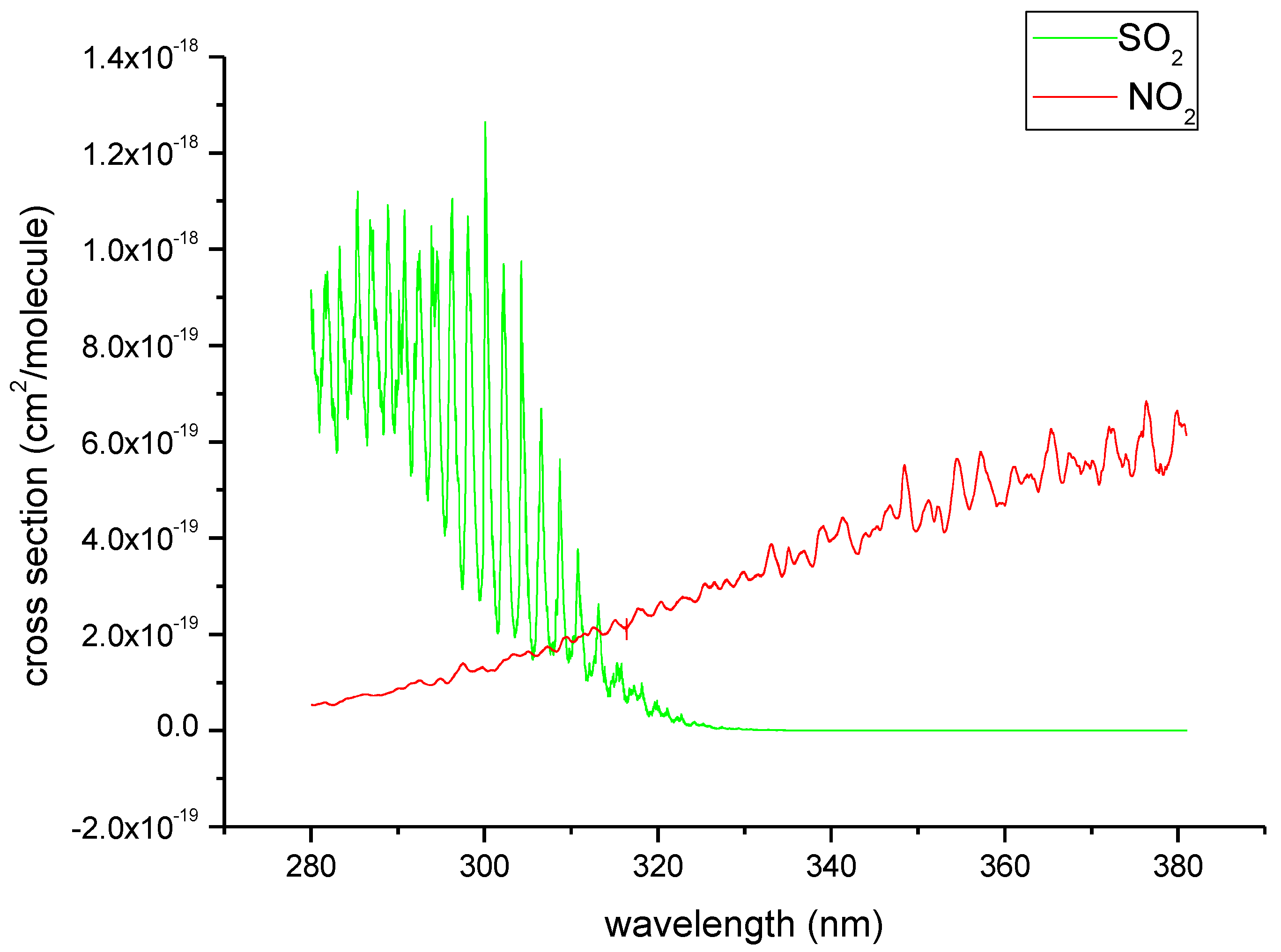
2.1. Single-Wavelength Simulation Analysis Model

The law of light absorption, also known as the Lambert–Beer law, is the theory of the quantitative analysis of the absorption effect of all light-absorbing substances, including molecules, atoms, ions, solids, liquids, and gases, on all electromagnetic radiation. The law of light absorption is expressed as follows [25]:

$$I(\lambda )=I_0(\lambda )\exp [-L(c_{S{O}_2}{\sigma }_{S{O}_2}(\lambda )+{\displaystyle \sum _{i=1}^n\sigma (\lambda )c_i})+{\epsilon }_R+{\epsilon }_M]$$

(1)

where I₀ is the initial light intensity; I is the light intensity received by the optical system after passing through the absorbing gas; L is the optical path length; λ is the wavelength; c_SO2 is the SO₂ concentration; σ_SO2(λ) is the SO₂ absorption cross-section for the given wavelength; c_i is the concentration of the other absorbing gases, excluding SO₂; σ_i(λ) is the absorption cross-section of the other absorbing gases; n is the number of the other types of absorbing gases; ${\epsilon }_R$ is the Rayleigh scattering; and ${\epsilon }_M$ is the Mie scattering.

In addition to the absorption effect of SO₂, NO₂ also has an obvious absorption cross-section in ship exhaust between 280 nm and 380 nm, as shown in Figure 1.

In this study, only the influence of NO₂ was considered, and the influence of scattering was ignored. Beecken J et al. [20] showed that between 15% and 50% of the NO emitted by ships is transformed into NO₂, and the specific value depends on the distance from the emission source. However, for the exhaust gas just out of the chimney mouth, the NO conversion rate may not reach 15%. Therefore, this study carried out a simulation analysis for 15 cases in which the NO conversion rate varied from 1% to 15%. The simulation analysis model was as follows:

$$I(\lambda )=I_0(\lambda )\exp [-L(c_{S{O}_2}{\sigma }_{S{O}_2}(\lambda )+c_{N{O}_2}{\sigma }_{N{O}_2}(\lambda ))]$$

(2)

According to Equation (2), the formula for calculating the SO₂ concentration can be expressed as follows after ignoring other gas absorption effects:

$$c_{S{O}_2}=[I_0(\lambda )/I(\lambda )]/[L\sigma (\lambda )]$$

(3)

The SO₂ absorption cross–sections of the three bands obtained from the High–Resolution Transmission Molecular Spectroscopy Database (HITRAN) were σ(300 nm) = 3.868 × 10⁻¹⁹ cm²/molecule, σ(310 nm) = 1.613 4 × 10⁻¹⁹ cm²/molecule, and σ(330 nm) = 4.797 × 10⁻²¹ cm²/molecule. In the previously stated form of the Lambert–Beer law, the unit of concentration of SO₂ was m²/g, so a unit conversion is required. The conversion formula is:

$${\sigma }_{{\mathrm{m}}^2/\mathrm{g}}=\frac{0.0001 {\mathrm{m}}^2/\mathrm{c}{\mathrm{m}}^2\ast {\sigma }_{\mathrm{c}{\mathrm{m}}^2/molecule}}{1.063\times {10}^{-22} \mathrm{g}/molecule}$$

(4)

As calculated by Equation (4), ${\sigma }_{300 }$ = 0.363876 m²/g, ${\sigma }_{310}$ = 0.15178 m²/g, and ${\sigma }_{330}$ = 0.0045127 m²/g. In the ship exhaust monitoring experiment, the diameter of the chimney was 0.8 m. Therefore, the three single-wavelength SO₂ concentration inversion models can be respectively expressed as:

$$c_{300}=3.435236\times \ln [\frac{I_0(300)}{I(300)}]$$

(5)

$$c_{310}=8.235604\times \ln [\frac{I_0(300)}{I(300)}]$$

(6)

$$c_{330}=276.996\times \ln [\frac{I_0(300)}{I(300)}]$$

(7)

Three error indicators; namely, root mean square error (RMSE), mean absolute error (MAE), and mean absolute percentage error (MAPE), were used to evaluate the accuracy of the SO₂ concentration calculation. The calculation methods of the three error indicators are presented below:

$$MAE=\frac{1}{k}{\displaystyle \sum _{i=1}^k\left|c_{true}-c_{forecast}\right|}$$

(8)

$$RMSE=\sqrt{\frac{1}{k}{\displaystyle \sum _{i=1}^k{\left|c_{true}-c_{forecast}\right|}^2}}$$

(9)

$$MAPE=\frac{1}{k}{\displaystyle \sum _{i=1}^k\left|\frac{c_{true}-c_{forecast}}{c_{true}}\right|}\times 100\%$$

(10)

where c_true is the true SO₂ concentration; c_forecast is the predicted SO₂ concentration; and k is the number of the groups of collected concentration data.

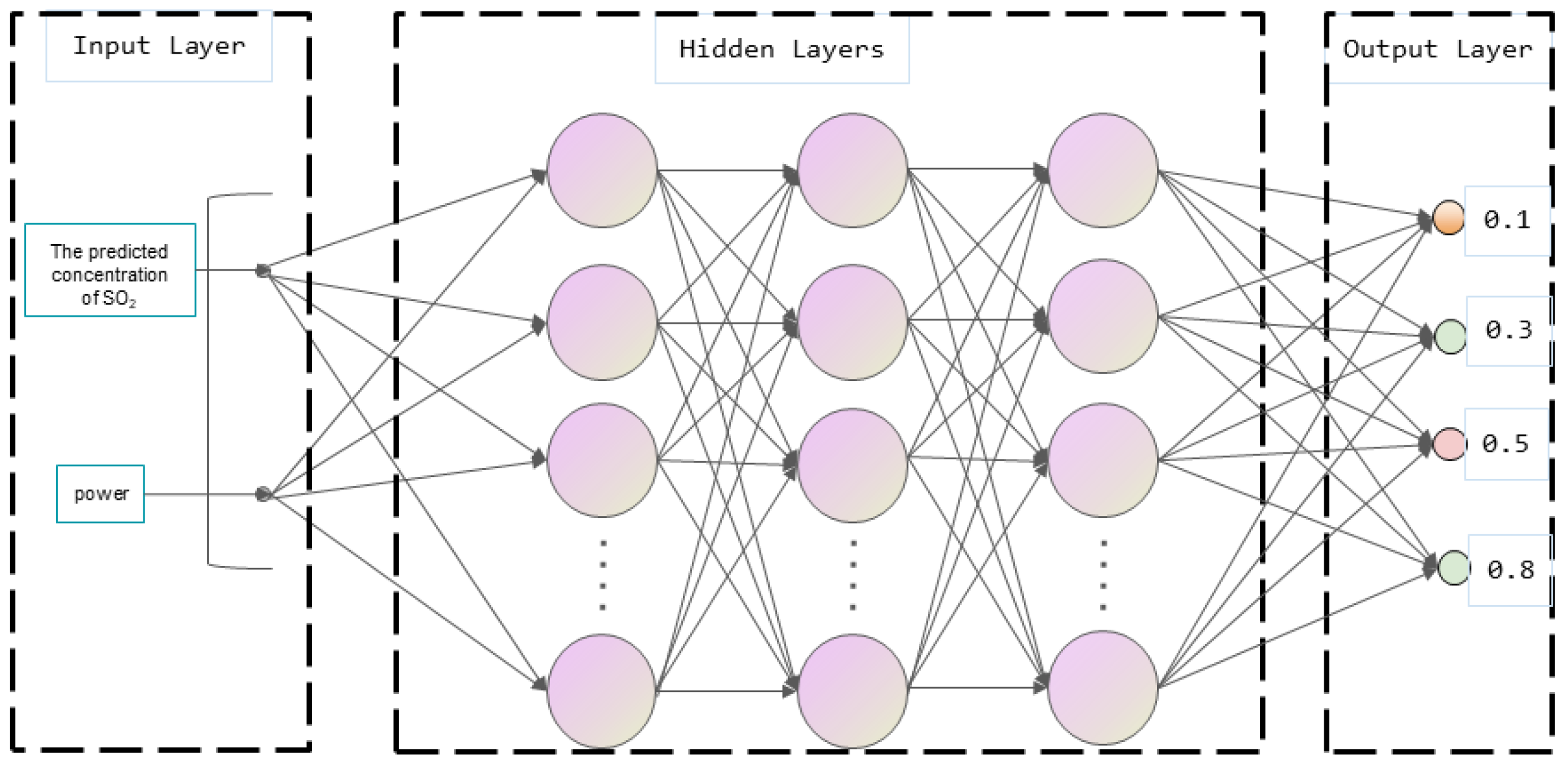
2.2. Deep Neural Network Model

Based on the SO₂ concentration obtained by inversion, a predictive model of sulfur content in ship oil was established using deep learning. However, the SO₂ concentration in ship exhaust will vary not only with fuel sulfur content, but also with engine power [27]. Thus, we needed to take the engine power into account. The sulfur content prediction model adopted the SO₂ concentration obtained from the inversion of the single-wavelength inversion model and the power of the main engine as the inputs to predict four different sulfur contents. The schematic diagram of the sulfur content prediction model is shown in Figure 2 below. Four types of marine fuel oil with sulfur contents of 0.1%, 0.3%, 0.5% and 0.8% were used in the experiment. Thus, the final output was one of the four sulfur contents.

3. Experiments and Data

A bench experiment utilizing UV imaging was performed to obtain the ship emission data closest to the actual situation and UV image data. Four types of fuel with a sulfur content ranging from 0.1 to 0.8% and 13 different engine power conditions ranging from 0 to 100% were used for this experiment. An online monitoring system was used to collect the gas concentration data by punching a hole in the flue, and UV imaging detection equipment was used to collect ultraviolet image data from the ship’s exhaust.

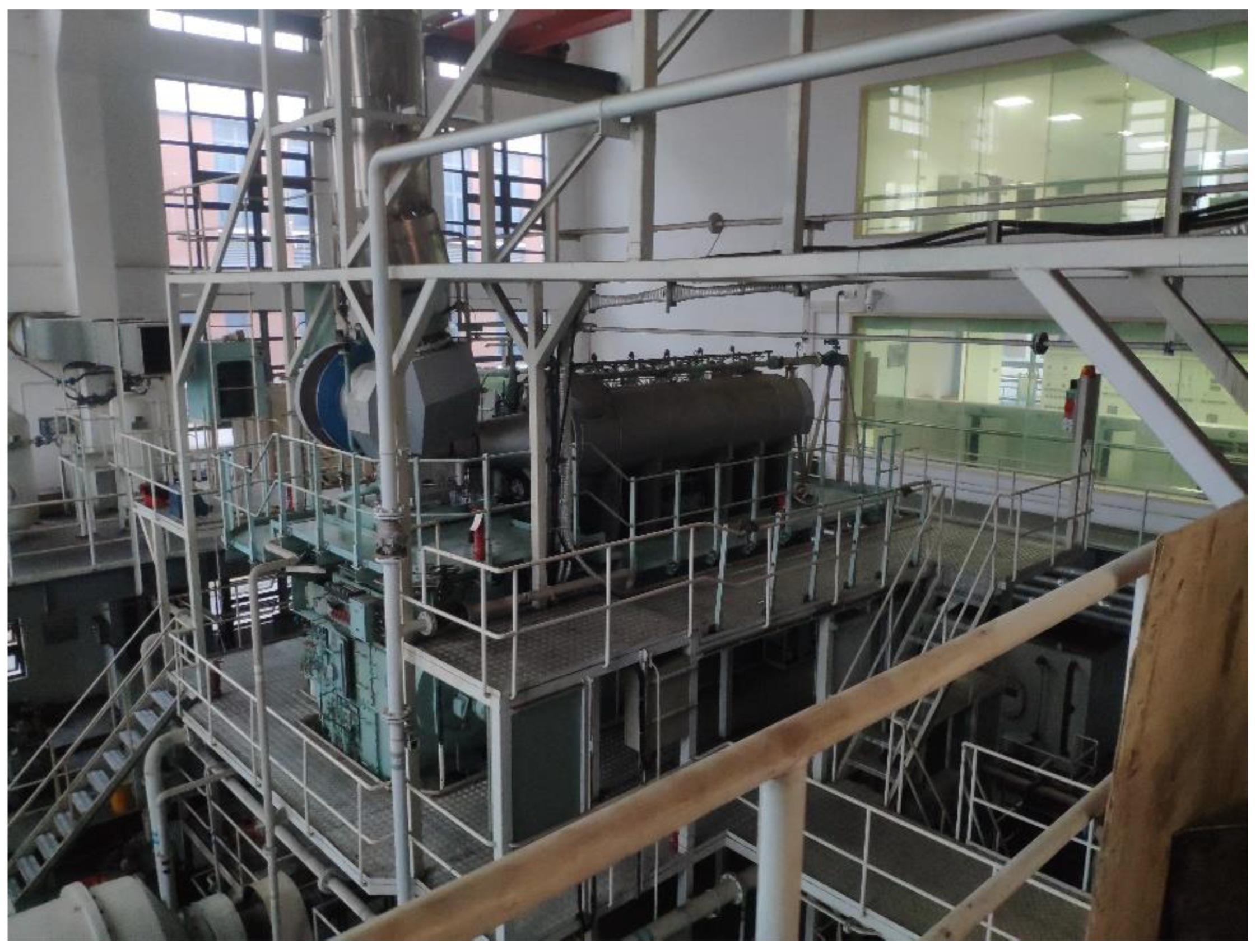
3.1. Experimental Diesel Engine

A MAN B&W 6S35ME-B9 diesel engine in Figure 3 was the main engine used in the bench experiment. It is an electronically controlled two-stroke six-cylinder cross-head-type ship main engine with 3400 kW power, 142 r/min rated speed, 3.5% allowable maximum marine fuel sulfur content, and 30,000 kg/h approved maximum tail gas handling capacity.

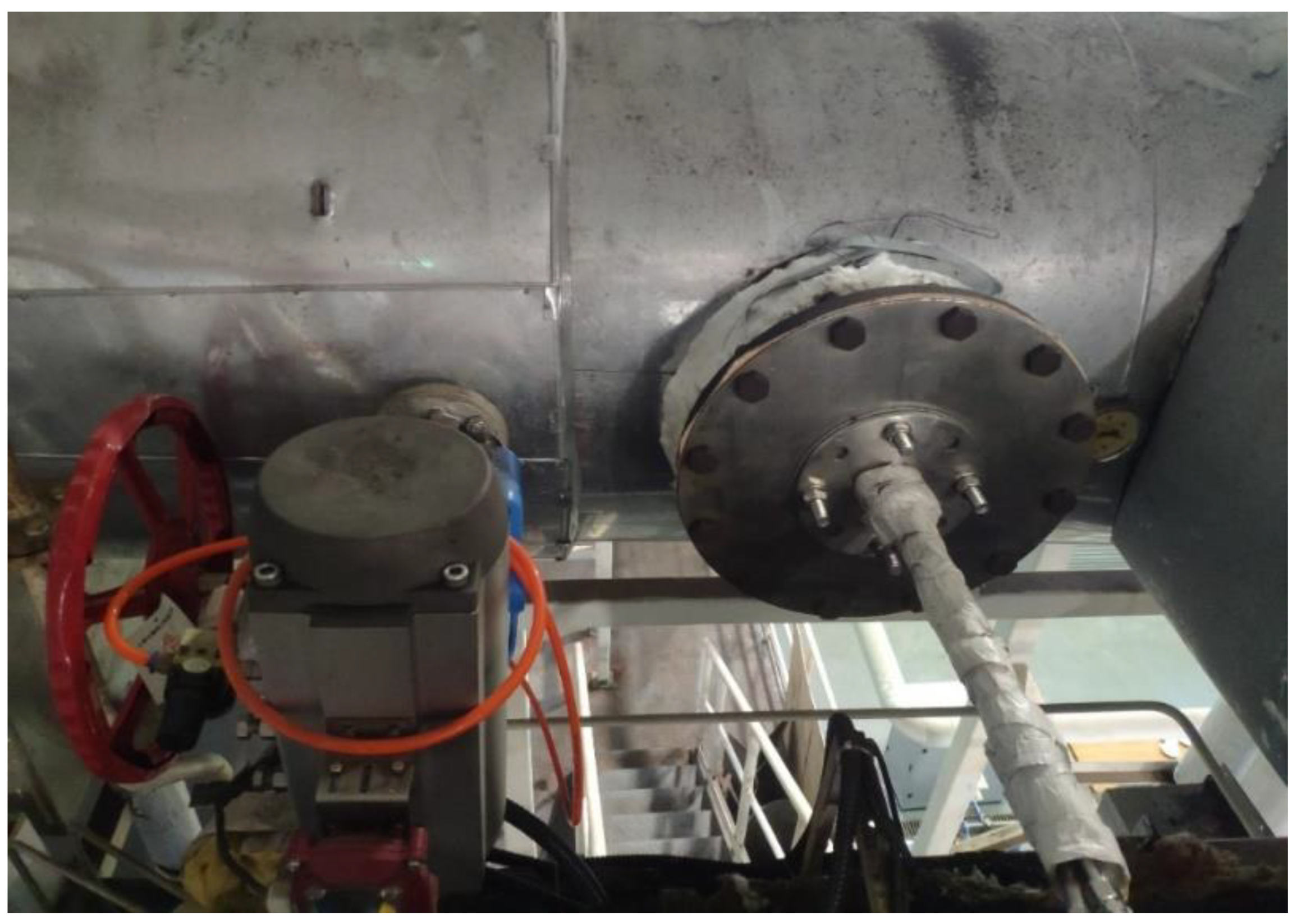
3.2. Online Monitoring Equipment

The sampling probe was placed in the center of the ship flue, and the real concentration of exhaust pollutants was determined by direct sampling of flue gas by using the ship exhaust online monitoring equipment. The connection between the sampling probe and the flue is shown in Figure 4.

An RJ-CEMD ship exhaust online monitoring system was selected; this system conforms to the MARPOL Annex VI and IMO–MEPC technical regulations on ship exhaust emissions.

3.3. Marine Fuel

Four types of marine fuel with sulfur contents of 0.1%, 0.3%, 0.5%, and 0.8% were used in the experiment. These were thought to be representative of the sulfur content in actual marine fuels used during navigation and berthing.

3.4. Working Conditions of the Diesel Engine

When marine fuel with the same sulfur content was used, the different working conditions of the diesel engine yielded the primary effect on the ship exhaust.

Table 1. Diesel engine conditions employed in the experiment.

Number	1	2	3	4	5	6	7	8	9	10	11	12	13
Power percentage (%)	0	5	10	15	20	25	30	40	50	60	80	90	100

shows the different working conditions of the diesel engine.

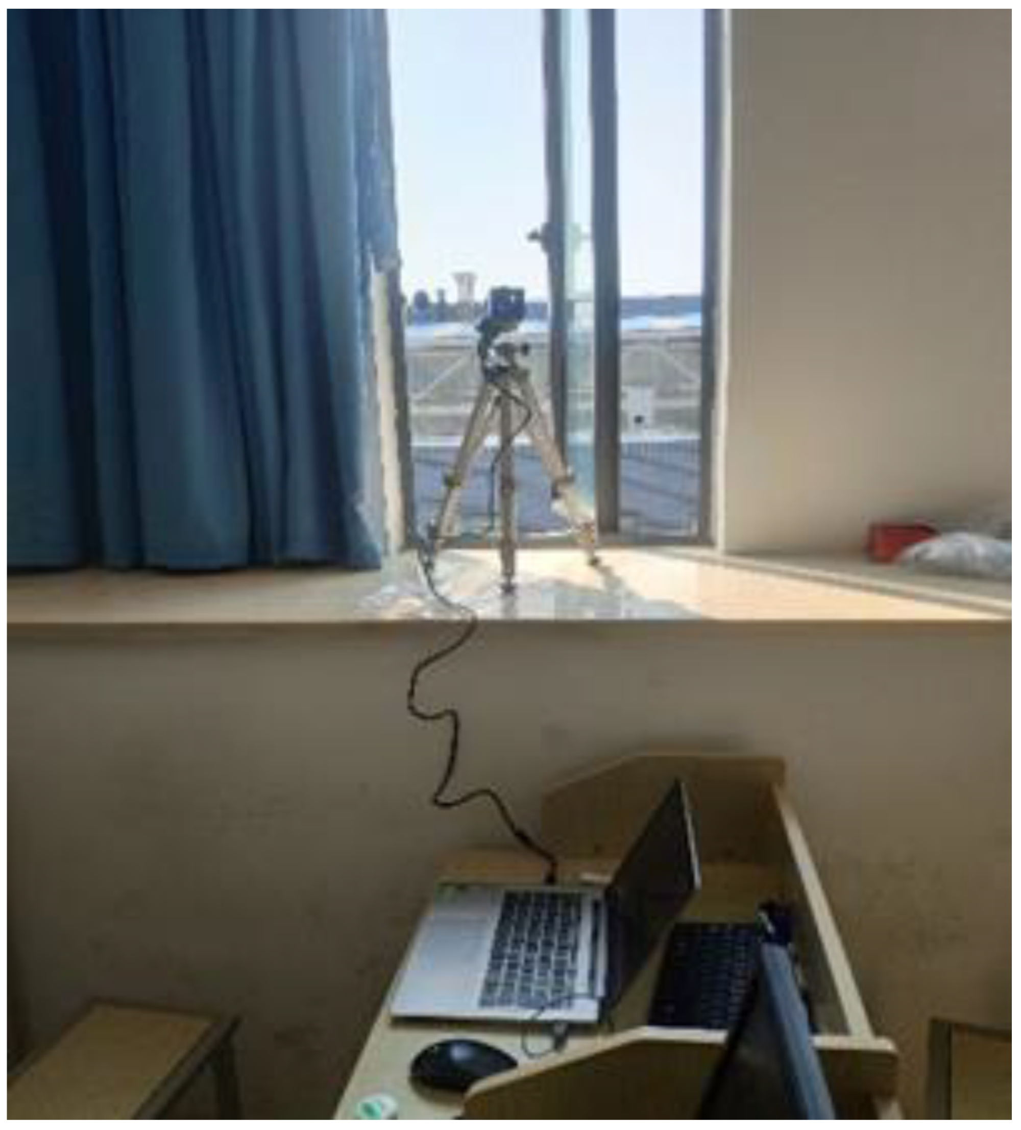
3.5. UV Imaging Detection Equipment

The ultraviolet imaging detection equipment used in this experiment is shown in Figure 5. The equipment had optical filter and measurement functions, and the spectral induction band was 230–920 nm. The working environment temperature range was −20 to 50 °C; the resolution was 2048 × 2048; the data bit depth was 16-bit; the focal length was 78 mm; and the lens size was 50 mm.

In order to minimize noise in the ultraviolet image and retain the detail of the image to the maximum extent, an adaptive fuzzy median filtering algorithm was used to filter the image. A square area with side lengths equal to 2/5 of the chimney diameter was selected for the extraction of ship exhaust. In order to ensure that SO₂ concentration was extracted from the same exhaust gas area in each image, a Canny edge-extraction algorithm was utilized to automatically extract the chimney boundary of each image, and then the location of ship exhaust gas area was found. The gray value in the extraction area was averaged and the background value subtracted to obtain the optical thickness needed to invert the concentration of SO₂.

4. Results and Discussion

4.1. Single-Wavelength Simulation Analysis Results

The collected gas concentration data were substituted into Equation (2) for the simulation, and then Equations (5)–(7) were used to obtain the respective inverted SO₂ concentrations. The single-wavelength simulation analysis results for different NO conversion rates at different wavelengths are shown in Figure 6.

When the tail gas was discharged from the flue, with the increase of the NO conversion rate, the interference from NO₂ was continuously enhanced, leading to the continuous increase of single-wavelength simulation errors. When the NO conversion rate was constant, the simulation errors at 300 nm were the smallest, because compared with the other two bands, the absorption of SO₂ at 300 nm was stronger, while the interference from NO₂ was smaller.

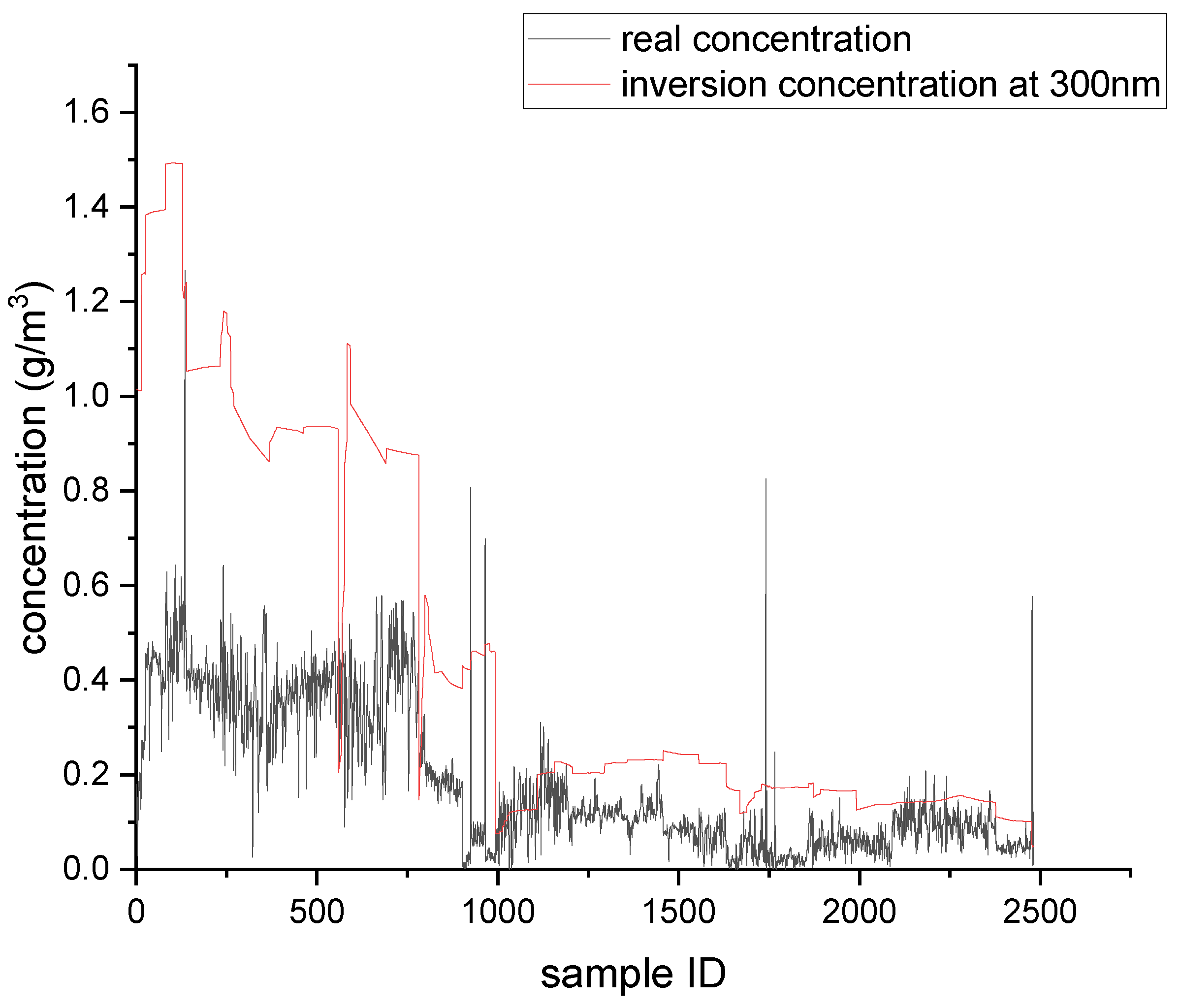
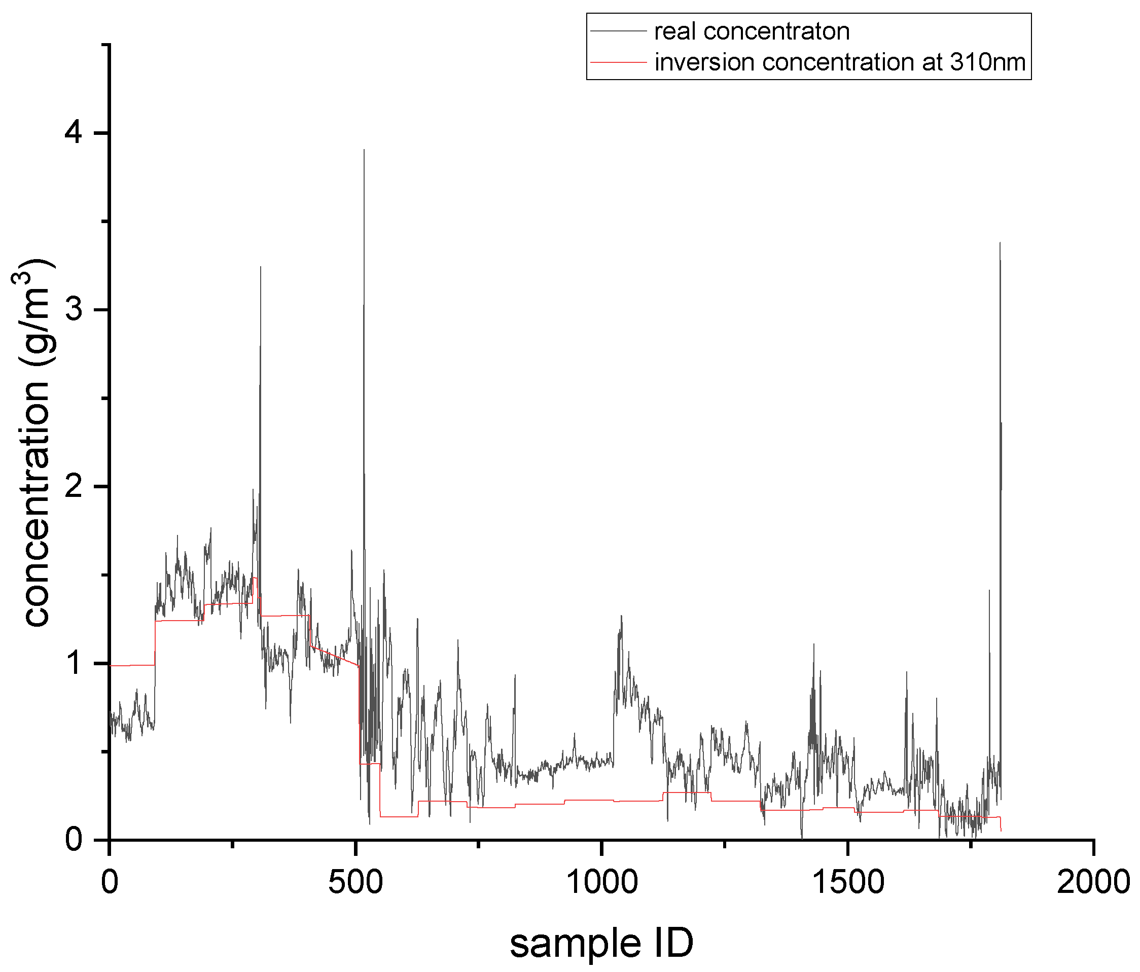
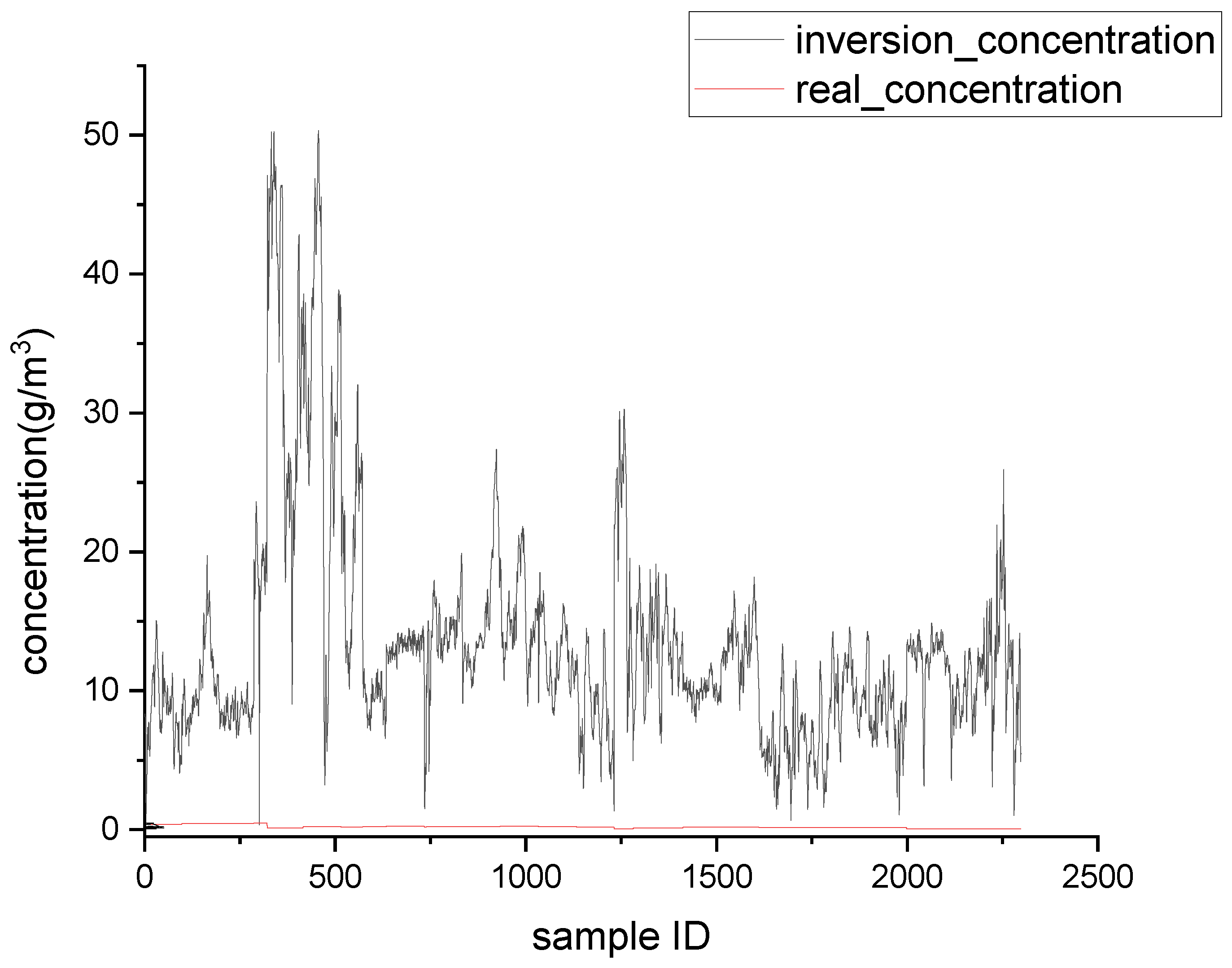
4.2. Single-Wavelength Inversion Results of Ultraviolet Images

Equations (5)–(7) were used to invert the collected ultraviolet images to obtain SO₂ concentration. The SO₂ concentration inversion results obtained from ultraviolet images at the three wavelengths are shown in Figure 7, Figure 8 and Figure 9.

The errors in SO₂ concentration inversion using UV images at the three wavelengths are shown in

Table 2. SO₂ concentration inversion errors at three UV wavelengths.

Wavelength (nm)	RMSE	MAE	MAPE
300	0.15	0.12	55.69
310	0.38	0.28	148.28
330	15.43	13.20	9976.35

.

As shown in Table 2, when the actual image was used for single-wavelength inversion, the minimum inversion errors occurred at 300 nm, which was consistent with the simulation results. This also was consistent with the fact that the absorption of SO₂ was the strongest at 300 nm, and the interference from NO₂ was the lowest at 300 nm.

By comparing the inversion results obtained from UV images with the simulation results, the conversion rate of NO just discharged from the chimney mouth was estimated to be approximately 7–8%. Regardless of the simulation results or the UV image inversion results, the errors at 330 nm were very large. This is because the absorption of SO₂ at 330 nm was very weak, while the interference factors such as absorption of NO₂ and scattering were very influential. In general, 330 nm is used as the reference channel in dual-wavelength inversion, and interference factors that do not change with wavelength are subtracted out, so as to obtain more accurate SO₂ concentration data. In this experiment, the real gas concentration was the gas concentration in the flue, while the UV image data collected was at the chimney mouth. Since it was impossible to know the dilution degree of the gas just coming out of the chimney mouth, it was assumed that the concentration of the gas just coming out of the flue mouth remained unchanged. In reality, the gas concentration at the flue mouth was lower than that in the flue. It can be seen from the inversion results for the three wavelengths that if the real SO₂ concentration was lowered, the inversion results at 300 nm were closer to the true value. Although 300 nm had the smallest inversion errors among the three wavelengths, it also had the highest requirement for skylight conditions in practical application. In the case of poor skylight background, the signal-to-noise ratio of a UV image acquired at 300 nm may be low, making the UV image data unusable. When the sulfur content was 0.1%, the concentration of SO₂ in the tail gas was low, and because the sensitivity of the detector used in this experiment was limited, most of the images collected at 300 and 310 nm could not be used due to low signal-to-noise ratios. However, at 330 nm, perhaps due to strong absorption of other gases and scattering, more effective data could be obtained. In future work, it will be necessary to consider the solar zenith angle, the transmittance curve of the filter, and other related factors, and to analyze the inversion errors of SO₂ concentration, the signal-to-noise ratio of the image, and other factors, so as to obtain the optimal detection wavelength for UV imaging technology.

4.3. Sulfur Content Prediction Results

Precision, recall, F1-score, accuracy, macro avg., and weighted avg. of the models were obtained by training with the data at the three respective wavelengths. The deep-learning results for the three wavelengths are shown in

Table 3. Model evaluation report for 300 nm.

Fuel Sulfur Content (% m/m)	Counts	Precision	Recall	F1-Score	Accuracy
0.1	4	0	0	0	-
0.3	806	0.71	0.81	0.76	-
0.5	676	0.74	0.69	0.72	-
0.8	212	0.81	0.57	0.66	-
Macro avg.	1698	0.57	0.52	0.54	-
Weighted avg.	1698	0.74	0.73	0.73	-
Total	1698	-	-	-	0.73

,

Table 4. Model evaluation report for 310 nm.

Fuel Sulfur Content (% m/m)	Counts	Precision	Recall	F1-Score	Accuracy
0.1	2	1	0.5	0.67	-
0.3	388	0.91	0.93	0.92	-
0.5	873	0.97	0.94	0.96	-
0.8	42	0.69	0.9	0.78	-
Macro avg.	1305	0.89	0.82	0.83	-
Weighted avg.	1305	0.94	0.94	0.94	-
Total	1305	-	-	-	0.94

and

Table 5. Model evaluation report for 330 nm.

Fuel Sulfur Content (% m/m)	Counts	Precision	Recall	F1-Score	Accuracy
0.1	300	0.49	0.49	0.49	-
0.3	767	0.74	0.83	0.78	-
0.5	910	0.81	0.76	0.79	-
0.8	321	0.60	0.53	0.56	-
Macro avg.	2298	0.66	0.65	0.65	-
Weighted avg.	2298	0.71	0.71	0.71	-
Total	2298	-	-	-	0.71

.

The prediction accuracy of sulfur content at 310 nm was the highest, reaching 94%. This indicated that the single-wavelength SO₂ inversion model combined with the deep-learning method could be used to accurately predict the sulfur content of ship fuel. The accuracy at 310 nm was the highest, possibly because the distribution characteristics of SO₂ inversion data at 310 nm conformed to the distribution characteristics of sulfur content, which was more easily learned by the deep neural network.

5. Conclusions

In this study, we performed a simulation experiment of ship exhaust emissions, built a single-wavelength simulation analysis model, and established a predictive model of sulfur content in ship fuel oil. The single-wavelength simulation analysis model could predict SO₂ concentration with high accuracy from an ultraviolet image of the exhaust plume taken by a UV camera. The predictive model of sulfur content resulted in the effective prediction of sulfur content of ship fuel oil. The results showed that the prediction accuracy of sulfur content was the highest at 310 nm, reaching 94%. This work proved the feasibility of using UV absorption characteristics of SO₂ to invert SO₂ concentration and then predict sulfur content in marine fuel oil combined with engine power. Our method could predict FSC without obtaining CO₂ or a model of the fuel consumption. This method could reduce the complexity of the equipment. As a result, the method is easy to use for marine fuel oil compliance inspection. In this paper, only the single-wavelength ship exhaust imaging detection method was studied. In future research, dual-wavelength ship exhaust imaging detection experiments will be carried out to establish a dual-wavelength ship exhaust SO₂ concentration prediction model, so as to provide more accurate SO₂ concentration prediction results. Furthermore, the deep neural network will be further improved to enhance the prediction accuracy of sulfur content in marine fuel oil.

References

1. Jalkanen, J.P.; Johansson, L.; Kukkonen, J. A comprehensive inventory of ship traffic exhaust emissions in the European sea areas in 2011. Atmos. Chem. Phys. 2016, 16, 71–84. [Google Scholar] [CrossRef] [Green Version]
2. International Maritime Organization. Reduction of GHG Emissions from Ships Third IMO GHG Study 2014—Final Report; MEPC.: London, UK, 2014; Volume 67. [Google Scholar]
3. International Maritime Organization (IMO). Annex VI of MARPOL 73/78, Regulations for the Prevention of Air Pollution from Ships and NOx Technical Code; IMO: London, UK, 2007; Volume 3, pp. 154–196. [Google Scholar]
4. Eyring, V.; Isaksen, I.S.A.; Berntsen, T.; Collins, W.J.; Corbett, J.J.; Endresen, O.; Grainger, R.G.; Moldanova, J.; Schlager, H.; Stevenson, D.S. Transport impacts on atmosphere and climate: Shipping. Atmos. Environ. 2010, 44, 4735–4771. [Google Scholar] [CrossRef]
5. Zhao, J.; Fan, J.; Zhang, B.; Shi, Y. Satellite remote-sensing monitoring technology and the research advances of SO2 in the atmosphere. J. Saf. Environ. 2012, 4, 166–169. [Google Scholar]
6. Yan, H.; Chen, L.; Tao, J.; Han, D.; Su, L.; Yu, C. SO2 long-term monitoring by satellite in the Pearl River Delta. J. Remote Sens. 2012, 2, 390–404. [Google Scholar]
7. Huaxiang, S.; Minhua, Y. Effectiveness evaluation of SO2 emission reduction in Guizhou Province. Earth Environ. 2014, 5, 319–327. [Google Scholar]
8. Huaxiang, S.; Minhua, Y. Analysis on effectiveness of SO2 emission reduction in Guangxi Zhuang Autonomous Region by satellite remote sensing. Chin. J. Environ. Eng. 2015, 3, 1361–1368. [Google Scholar]
9. Li, B.; Ju, T.; Zhang, B.; Ge, J.; Zhang, J.; Tang, H. Satellite remote sensing monitoring and analysis of the causes of temporal and spatial variation characteristics of atmospheric SO2 Concentration in Tianshui. Environ. Monit. China 2016, 2, 134–140. [Google Scholar]
10. Li, C. Emissions Characteristics and Future Trends of Non-Road Mobile Sources in China. Ph.D. Thesis, South China University of Technology, Guangzhou, China, 2017. [Google Scholar]
11. Mellqvist, J.; Conde, V.; Beecken, J.; Ekholm, J. Surveillance of Sulfur Emissions from Ships in Danish Waters; Chalmers University of Technology: Göteborg, Sweden, 2017. [Google Scholar]
12. Daniel, A.B.; Carmen, R.M.B. Bridge-based sensing of NOx and SO2 emissions from ocean-going ships. Atmos. Environ. 2016, 136, 54–60. [Google Scholar]
13. Zhou, F.; Pan, S.; Chen, W.; Ni, X.; An, B. Monitoring of compliance with fuel sulfur content regulations through unmanned aerial vehicle (UAV) measurements of ship emissions. Atmos. Meas. Tech. 2019, 12, 6113–6124. [Google Scholar] [CrossRef] [Green Version]
14. Anand, A.; Wei, P.; Gali, N.K.; Sun, L.; Yang, F.; Westerdahl, D.; Zhang, Q.; Deng, Z.; Wang, Y.; Liu, D.; et al. Protocol development for real-time ship fuel sulfur content determination using drone based plume sniffing microsensor system. Sci. Total Environ. 2020, 744, 140885. [Google Scholar] [CrossRef]
15. Seyler, A.; Wittrock, F.; Kattner, L.; Mathieu-Üffing, B.; Peters, E.; Richter, A.; Schmoke, S.; Burrows, J.P. Monitoring shipping emissions in the German Bight using MAX-DOAS measurements. Atmos. Chem. Phys. 2017, 17, 10997–11023. [Google Scholar] [CrossRef] [Green Version]
16. Berg, N.; Mellqvist, J.; Jalkanen, J.P.; Balzani, J. Ship emissions of SO2 and NO2: DOAS measurements from airborne platforms. Atmos. Meas. Tech. 2012, 5, 1085–1098. [Google Scholar] [CrossRef] [Green Version]
17. Cheng, Y.; Wang, S.; Zhu, J.; Guo, Y.; Zhang, R.; Liu, Y.; Zhang, Y.; Yu, Q.; Ma, W.; Zhou, B. Surveillance of SO2 and NO2 from ship emissions by MAX-DOAS measurements and implication to compliance of fuel sulfur content. Atmos. Chem. Phys. 2019, 19, 13611–13626. [Google Scholar] [CrossRef] [Green Version]
18. Prata, A.J. Measuring SO2 ship emissions with an ultraviolet imaging camera. Atmos. Meas. Tech. 2014, 7, 1213–1229. [Google Scholar] [CrossRef] [Green Version]
19. Osorio, M.; Casaballe, N.; Belsterli, G.; Barreto, M.; Gomez, A.; Ferrari, J.A.; Frins, E. Plume segmentation from UV camera images for SO2 emission rate quantification on cloud days. Remote. Sens. 2017, 9, 517. [Google Scholar] [CrossRef] [Green Version]
20. Beecken, J.; Mellqvist, J.; Salo, K.; Ekholm, J.; Jalkanen, J.-P. Airborne emission measurements of SO2, NOx and particles from individual ships using a sniffer technique. Atmos. Meas. Tech. 2014, 7, 1957–1968. [Google Scholar] [CrossRef]
21. Premuda, M.; Masieri, S.; Bortoli, D.; Kostadinov, I.; Petritoli, A.; Giovanelli, G. Evaluation of vessel emissions in a lagoon area with ground based Multi axis DOAS measurements. Atmos. Environ. 2011, 45, 5212–5219. [Google Scholar] [CrossRef]
22. Balzani Lööv, J.M.; Alfoldy, B.; Gast, L.F.L.; Hjorth, J.; Lagler, F.; Mellqvist, J.; Beecken, J.; Berg, N.; Duyzer, J.; Westrate, H.; et al. Field test of available methods to measure remotely SOx and Nox emissions from ships. Atmos. Meas. Tech. 2014, 7, 2597–2613. [Google Scholar] [CrossRef] [Green Version]
23. Zhou, F.; Gu, J.; Chen, W.; Ni, X. Measurement of SO2 and NO2 in ship plumes using rotary unmanned aerial system. Atmosphere 2019, 10, 657. [Google Scholar] [CrossRef] [Green Version]
24. Duan, W.; Xiong, Y.; Chen, Z.; Yu, G.; Liu, L.; Li, F.; Wu, K. Remote sensing and monitoring of industrial SO2 and carbon black particles with ultraviolet imaging technology. Acta Photonica Sin. 2020, 49, 153–161. [Google Scholar]
25. Zhang, Z.; Zheng, W.; Cao, K.; Li, Y.; Xie, M. Simulation analysis on the optimal imaging detection wavelength of SO2 concentration in ship exhaust. Atmosphere 2020, 11, 1119. [Google Scholar] [CrossRef]
26. Gordon, I.E.; Rothman, L.S.; Hill, C.; Kochanov, R.V.; Tan, Y.; Bernath, P.F.; Birk, M.; Boudon, V.; Campargue, A.; Chance, K.V.; et al. The HITRAN 2016 molecular spectroscopic database. J. Quant. Spectrosc. Radiat. Transf. 2017, 203, 3–69. [Google Scholar] [CrossRef]
27. Cao, K.; Zhang, Z.; Li, Y.; Zheng, W.; Xie, M. Ship fuel sulfur content prediction based on convolutional neural network and ultraviolet camera images. Environ. Pollut. 2021, 273, 116501. [Google Scholar] [CrossRef]
Figure 1. SO2 and NO2 absorption cross-sections (data source: the HITRAN 2016 molecular spectroscopic database [26]).
Atmosphere 12 01182 g001
Figure 2. The schematic diagram of the sulfur content prediction model.
Atmosphere 12 01182 g002
Figure 3. Ship diesel engine selected for the experiment.
Atmosphere 12 01182 g003
Figure 4. Sampling port of the chimney channel.
Atmosphere 12 01182 g004
Figure 5. UV detection equipment for plume sampling.
Atmosphere 12 01182 g005
Figure 6. Single-wavelength simulation analysis results for different NO conversion rates at different wavelengths.
Atmosphere 12 01182 g006
Figure 7. Single-wavelength inversion results at 300 nm.
Atmosphere 12 01182 g007
Figure 8. Single-wavelength inversion results at 310 nm.
Atmosphere 12 01182 g008
Figure 9. Single-wavelength inversion results at 330 nm.
Atmosphere 12 01182 g009