Abstract
Increasingly stringent environmental requirements for marine engines imposed by the International Maritime Organisation and the European Union require that marine engines have the lowest possible emissions of greenhouse and harmful exhaust gases into the atmosphere. In this research, exhaust gas emissions were measured on three Ro-Pax vessels sailing in the Adriatic Sea. Testo 350 Maritime exhaust gas analyser was used for monitoring the dry exhaust gas concentrations of CO2 and O2 in percentage, concentrations of CO and NOx in ppm and exhaust gas temperature in °C after the turbocharger at different engine loads. In order to compare and validate measured values, exhaust gas measurement data were also obtained from a Wartsila-Transas simulator model of a similar Ro-Pax vessel during the joint operation of the engine room and navigational simulators. All analysed main engines on three vessels had complete combustion processes in the cylinders with small differences which should be further investigated. Comparison of on board measured parameters with simulated parameters showed that significant fuel oil reduction per voyage could be accomplished by voyage and/or engine operation optimization procedures. Results of this analysis could be used for creating additional emission database and data-driven models for further analysis and improved estimation of exhaust gasses under various marine engine conditions. Additionally, the results could be useful to all interested parties in reducing the fuel oil consumption and emissions of greenhouse and harmful exhaust gases from vessels into the atmosphere.
1. Introduction
International and domestic shipping is a growing source of exhaust gas pollutants and greenhouse gas emissions. This problem was recognized by the European Union (EU) and they approved Regulation 2015/757 of the European Parliament and of the Council on the monitoring, reporting and verification of CO2 emissions from maritime transport [1]. The goal of the EU Commission is to limit the greenhouse gases on board by 2% in 2025 and up to 6% in 2030 compared with 2020 levels. This regulation includes monitoring and reporting CO2 emissions in the European Economic Area (EEA) from ships larger than 5000 gross tonnage (GT). According to the European Maritime Safety Agency (EMSA), companies should submit their emission report through the THETIS-MRV web platform [2]. This database was used to analyse CO2 emissions in 2018 from Ro-Pax vessels calling at European ports [3]. International Maritime Organization (IMO) followed this example with the IMO Data Collection System module which requires ships larger than 5000 GT to report and record fuel oil consumption [4]. The mentioned regulations and amendments are the first steps to develop the strategy for the decarbonizing maritime sector.
To evaluate the amount of emissions in one shipping area or from a specific type of ship is not an easy task. The most accurate method for estimating ship exhaust emissions is by on board measuring in real conditions with adequate measuring equipment. Thus far, research studies on the on board emissions measurement, especially in the Ro-Pax segment, are very limited. This problem presents a need for a more relevant onboard emission database that will offer the possibility to enhance the estimation of emissions and comparison with the current emission database and current estimation models.
Cooper D.A. measured exhaust emissions on high-speed passenger ferries with different propulsion types (conventional diesel engine, gas turbine, diesel engine with selective catalytic reduction) and at three most frequent engine loads [5]. The proposed method to quantify exhaust emissions without direct measurement of fuel consumption during manoeuvring is presented in [6]. An improved emission inventory method is suggested in [7] considering experimental on board measurement on two ocean going vessels with slow speed diesel engines using the heavy fuel oil (HFO). Another on board measurement research [8] was carried out on a slow speed, two stroke main engine running on HFO (3.13% sulphur content) with the goal to predict primary emissions while cruising, manoeuvring and at berth operating mode. Similar studies [9,10,11,12] have used equipment to measure the concentration of NOX, CO2, CO, SO2 and particulate matter (PM) pollutants in burned HFO, with respect to engine power output and vessel speed at different operating conditions. In [13], the comparison of fuel-based emission factors (NOX, PM, HC, CO) for different engine loads is presented with a conclusion that emission factors are increasing due to higher engine loads. Most of the vessel types in the previously mentioned literature are bulk carriers, container ships or general cargo ships with slow speed two stroke engines using the HFO. However, all researchers share the same opinion and conclusion that there should be more experimental measured data acquired under real seagoing conditions to provide development and validation of more relevant emission factors.
The aim of this paper is to compare and validate exhaust gas emissions data from onboard measurements with simulated data. The measurement campaign was performed on three similar Ro-Pax vessels, and simulation was performed in a joint operation of the Wartsila-Transas engine room and navigational simulators with Ro-Pax vessel models.
2. An Overview of Combustion Process and Exhaust Gases
Fuel oil for marine diesel engines mainly consists of carbon, hydrogen and sulphur (C, H, and S). Fuel oil is mixed with air and burned inside the cylinders. The products of the combustion process are exhaust gases (Figure 1), which are led to the atmosphere after their heat energy is used for power generation in the marine engines.
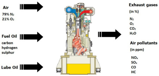
Figure 1.
Combustion process in engines.
For complete combustion of fuel oil comprising of carbon, hydrogen and sulphur, the total volume or mass of exhaust gases per kg of burned fuel oil can be calculated according to [14]:
Total volume or mass of dry exhaust gases is then calculated as:
For an amount of carbon, c [kg C/kg fuel], hydrogen, h [kg H/kg fuel] and sulphur, s [kg S/kg fuel] in fuel oil, the volume () or mass () of each exhaust gas can be calculated as follows [15]:
where the minimum amount of oxygen required for complete combustion of fuel can be calculated as [16]:
and minimum or stoichiometric amount of air as [16]:
Usually, in the actual combustion process, more air than the stoichiometric amount is used in order to increase the chances of complete combustion. The amount of excess air expressed as a ratio between the actual amount of air and the minimum or stoichiometric amount of air is obtained with the equation [17,18]:
Additionally, in the actual combustion process, there could be gases present in parts per million (ppm) like NOx, CO and other. The emission factor of each gas is converted into g/kWh units, which represent mass per kWh of engine work. For gases measured in ppm, the emission factors are obtained with the following equation [19]:
where and are relative molecular weight of particular gas and exhaust gas mixture in kmol/kg, respectively, is gaseous concentration in ppm in dry or wet gases, is dry or wet exhaust gas flow in kg/h and is the engine power.
To calculate the precise amount of exhaust gas (or exhaust flow) it is necessary to know the exact chemical properties of used fuel oil. The fuel oil properties used in this research are in correspondence with ISO 8217 2017 fuel standards for marine distillate fuels [20]. The amount of sulphur content in fuel must not exceed 0.10% by mass in all EU ports and inland waters, which is defined by EU directive 2016/802 [21].
3. On Board Measurement and Simulation Process
On board exhaust gas measurements were carried out on three Ro-Pax vessels with four stroke main engines connected through reduction gearboxes to controllable pitch propellers (CPP) during multiple voyages in the Adriatic Sea between ports of Croatia, Italy and Montenegro. In order to compare the on board measurement values of the exhaust process with the simulated ones and in addition to perform the validation of the engine room simulator with the measured on board values under a series of different engine operating regimes, the simulated exhaust gas data were also obtained using a Wartsila-Transas simulator model of similar Ro-Pax vessel. The simulated vessel was operated in a joint operation of the engine room and navigational simulators during different weather and engine operating conditions. The basic vessels’ and simulator’s particulars/parameters are shown in Table 1.

Table 1.
Vessel and engine particulars/parameters.
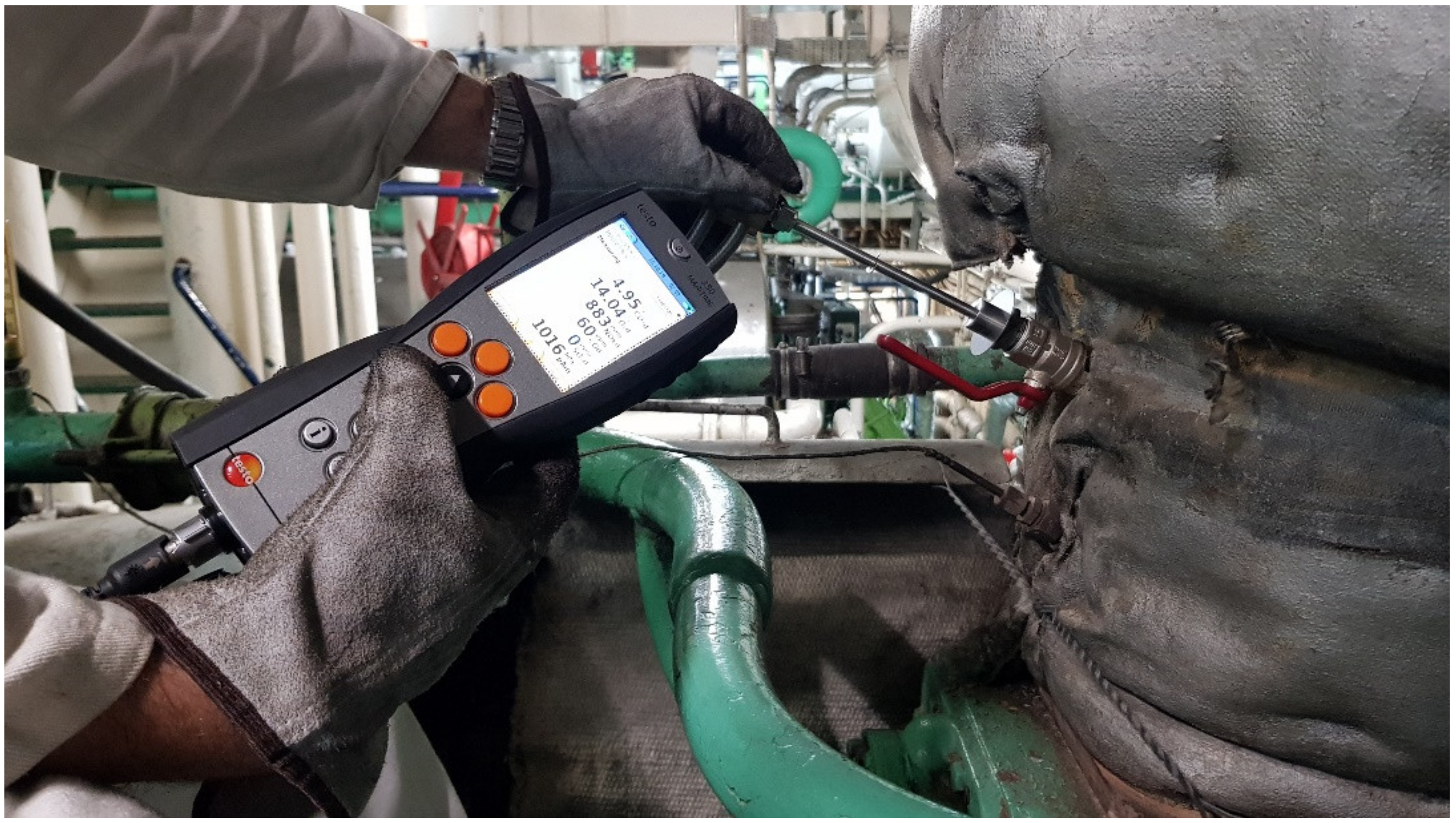
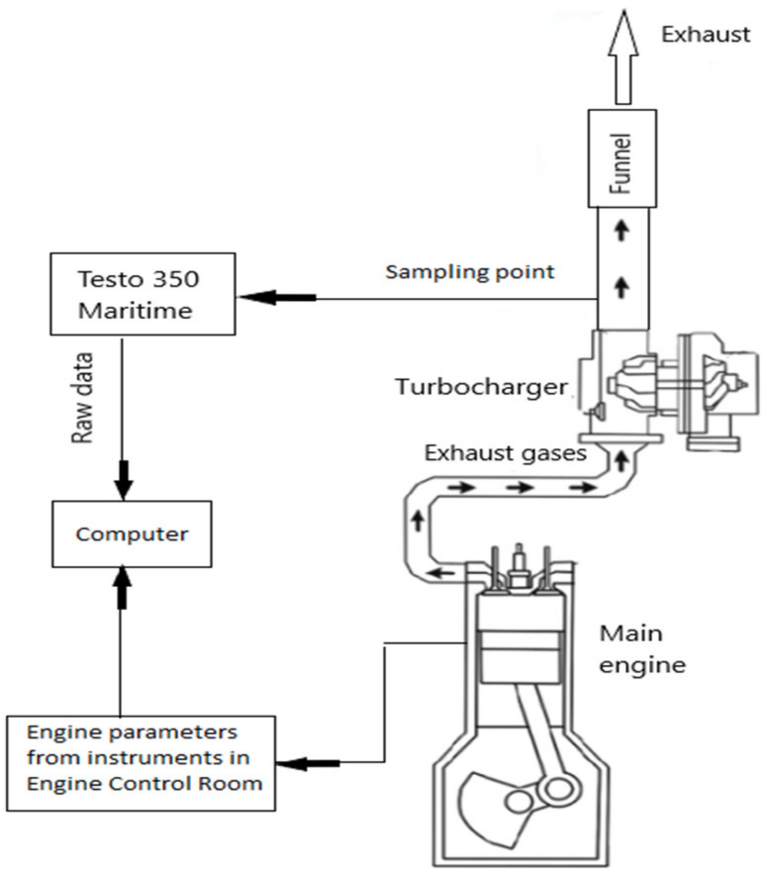
The equipment used for measuring and analysing the exhaust gases on board vessels was Testo 350 Maritime flue gas analyser [22]. This flue gas analyser is used for monitoring exhaust gas temperature and concentrations of CO2 and O2 as a percentage in volume of dry exhaust gas, as well as CO, NOx, SOx in ppm in dry exhaust gas. It is working in accordance with ISO 8178-4:2020, Marpol Annex VI and NOx Technical Code 2008. The measurement range and accuracy of the exhaust gas analyser can be found in [23]. The measured raw data files are saved into the analyser internal memory with an option to transfer it to the computer and then use for the analysis. On all three vessels diesel fuel Eurodiesel BS with a maximum of 10 mg/kg of sulphur content was used, which is also in conformity with Regulation 14(1) or 4(a) and Regulation 18(1) of Annex VI [24].
The onboard measuring process was carried out during the cruising phase of the voyages. For collecting the exhaust gas samples every few minutes during a period of one hour, the measuring equipment connection point located after the turbine wheel, in the exhaust duct, was used. The probe hole was adjusted with a small ball valve (Figure 2), which was located approximately 0.2 m downstream from the turbocharger.

Figure 2.
Sampling point located after the turbocharger.
The scheme of the flue gas analyser setup for the main engine exhaust gas measurement is shown in Figure 3. All other relevant engine/vessel parameters for this analysis were also collected directly from instruments in the engine control room and navigational bridge during the measuring processes.
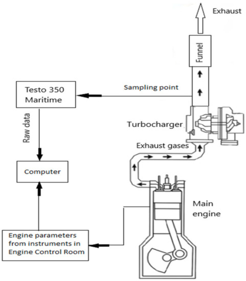
Figure 3.
Scheme of measuring equipment setup.
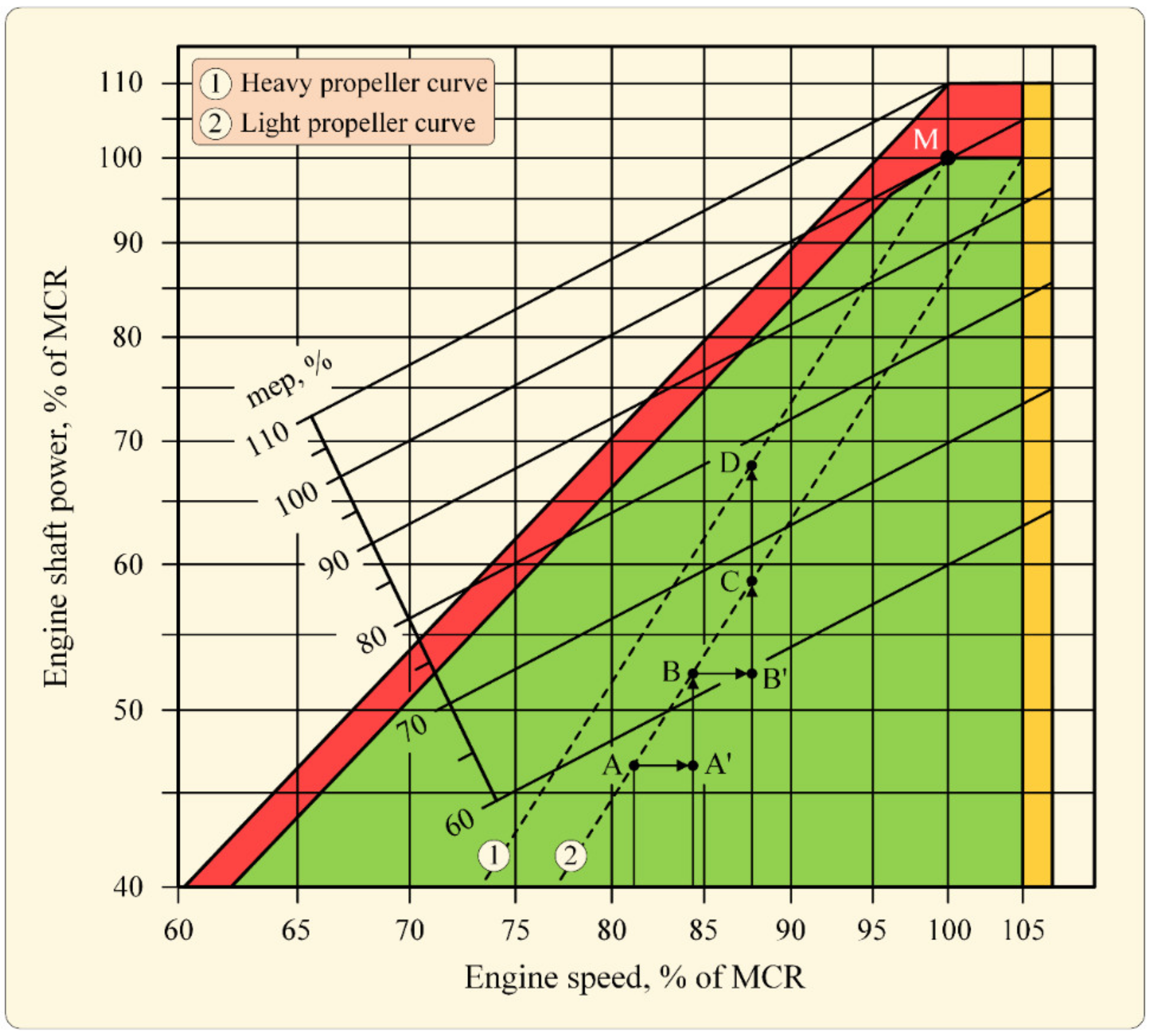
Standard engine load diagram for controllable pitch propeller with combinator mode presented in logarithmic scale is shown in Figure 4. During the combinator mode on, both engine speed and respective propeller pitch are changed according to the combinator (propeller) curve during the acceleration or deceleration of an engine. With light combinator (propeller) curve 2 the engine speed is increased, for example, from point A to point A′ before the propeller pitch is increased from point A′ to point B. If the engine speed has to be decreased, first the propeller pitch is reduced, for example, from point C to B′, and then the engine speed is reduced from point B′ to B. Normally, the main engine could work with heavy combinator (propeller) curve 1 during heavy weather, hull fouling or when vessel is loaded. If the engine speed (and propeller pitch) is kept constant (for example, with the telegraph lever in the same position) in point C, with designated engine shaft power and mean effective pressure (mep) inside the cylinders, then all excess load on the propeller and main engine because of the heavy weather will result in a change of combinator curve. This will cause an increase of engine shaft power and mean effective pressure inside the cylinders to point D. The engine operating point should never be in the red coloured engine overloaded area of the diagram which is at the top of the diagram defined by the maximum continuous rating (MCR) point M.

Figure 4.
Standard engine load diagram for CPP propeller.
One example of vessels’ controllable pitch propeller combinator working principle is shown in Figure 5. A signal from the engine telegraph lever is supplied to the CPP control system. If the engine has to be started ahead, the engine telegraph lever has to be moved to the position larger than 2 on the x-axis. Any ahead movement of the engine telegraph lever to a position from 2 to 7 will increase the engine speed (blue line) and consequently increase the percentage of propeller pitch (red dashed line). Any ahead movement of the telegraph lever to a position from 7 to 10 will not increase the engine speed (it will be constant), but it will increase the percentage of propeller pitch, and thus the engine load. Similar action will result during the astern movement of the engine telegraph lever, i.e., for negative values of the lever position.
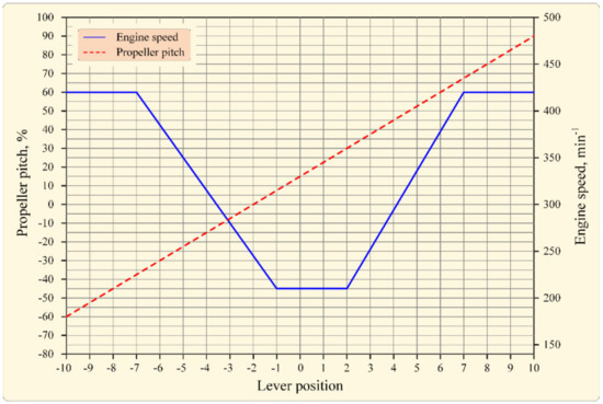
Figure 5.
Example of CPP propeller combinator working principle.
All three vessels sailed overnight back-to-back voyages between ports of Croatia and Italy. Only one vessel had one voyage between Italy and Montenegro. Voyage durations were from 9 to 11 h and exhaust gas measurements were taken 5–10 times per hour. Vessel 1 has four main engines connected in pair to two controllable pitch propellers (Figure 6). On each voyage vessel operated with only two main engines (one port and one starboard) propelling the both controllable pitch propellers. On the return voyage the engines were replaced with other two that were not running the night before. Layouts of propulsion systems on all three vessels are shown in Figure 6. Vessel 1 exhaust gas measurements were taken during the four back-to-back voyages (8 nights/days) and 235 exhaust gas measurement records were collected for this analysis. The average length of the voyages for Vessel 1 was 136.7 Nm, average speed 13.4 knots, average vessel heading was 260° when sailing from Croatia to Italy and 99° when sailing from Italy to Croatia. During the voyages average absolute wind direction with respect to true North was 128° with the average speed of 8.3 m/s and a sea condition of 5, according to the Beaufort scale.
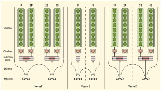
Figure 6.
Layouts of propulsion systems.
Vessel 2 has two main engines (port and starboard) each connected to its controllable pitch propeller. On each voyage, the vessel operated with both main engines propelling the two controllable pitch propellers, but for some short periods, the vessel sailed with only one engine/propeller (port or starboard). Vessel 2 exhaust gas measurements were taken during the one back-to-back voyage (2 nights/days), and 99 exhaust gas measurement records were collected for this analysis. The average length of the voyages for Vessel 2 was 102.6 Nm, average speed 11.6 knots, and average vessel heading was 245° when sailing from Croatia to Italy and 65° when sailing from Italy to Croatia. During the voyages, average absolute wind direction with respect to true North was 189° with the average speed of 3.2 m/s and a sea condition of 2, according to the Beaufort scale.
Vessel 3 has four main engines connected in pair to two controllable pitch propellers, similar to Vessel 1. On each voyage, the vessel operated with two main engines connected to only one (port or starboard) controllable pitch propeller. On the return voyage, the engines and propeller were replaced with other two engines and (port or starboard) propeller that were not running the night before. Vessel 3 exhaust gas measurements were also taken during the one back-to-back voyage (2 nights/days) and 153 exhaust gas measurement records were collected for this analysis. The average length of the voyages for Vessel 3 was 115 Nm, average speed 12.1 knots and average vessel heading was 210° when sailing from Croatia to Italy and 61° when sailing from Italy to Montenegro. During the voyages, average absolute wind direction with respect to true North was 167° with the average speed of 3.0 m/s and a sea condition of 2, according to the Beaufort scale.
The recorded output variables from Testo 350 Maritime flue gas analyser, presented in Table 2, were: concentration of CO2 and O2 as a percentage in a volume of dry (d) exhaust gas, concentrations of CO and NOX in ppm in dry exhaust gas and exhaust gas temperature after the turbocharger. The engine shaft power as a percentage of maximum continuous rating (MCR), at which measurements were taken, was calculated according to the parameters collected directly from the instruments in the engine room. Table 2 also shows basic statistics (mean μ and standard deviation σ) of measured and analysed dry exhaust gas quantities for all three vessels and their associated engines with calculated average values. During the voyage the engine speed and main engines load were varied according to the existing weather conditions and/or required vessel speed. All of that influenced the engine shaft power/load, as previously explained and shown in Figure 4.
Table 2.
Basic statistics (mean μ and standard deviation σ) of measured and analysed quantities for all vessels and their associated port (P) and starboard (S) engines with calculated average values.
Standard deviation σ used in this analysis is based on a normalization factor of N, i.e., it can be defined as:
where N denotes a number of measurements for the associated measurement sample, is the i-th measurement, and μ represents the mean value defined as:
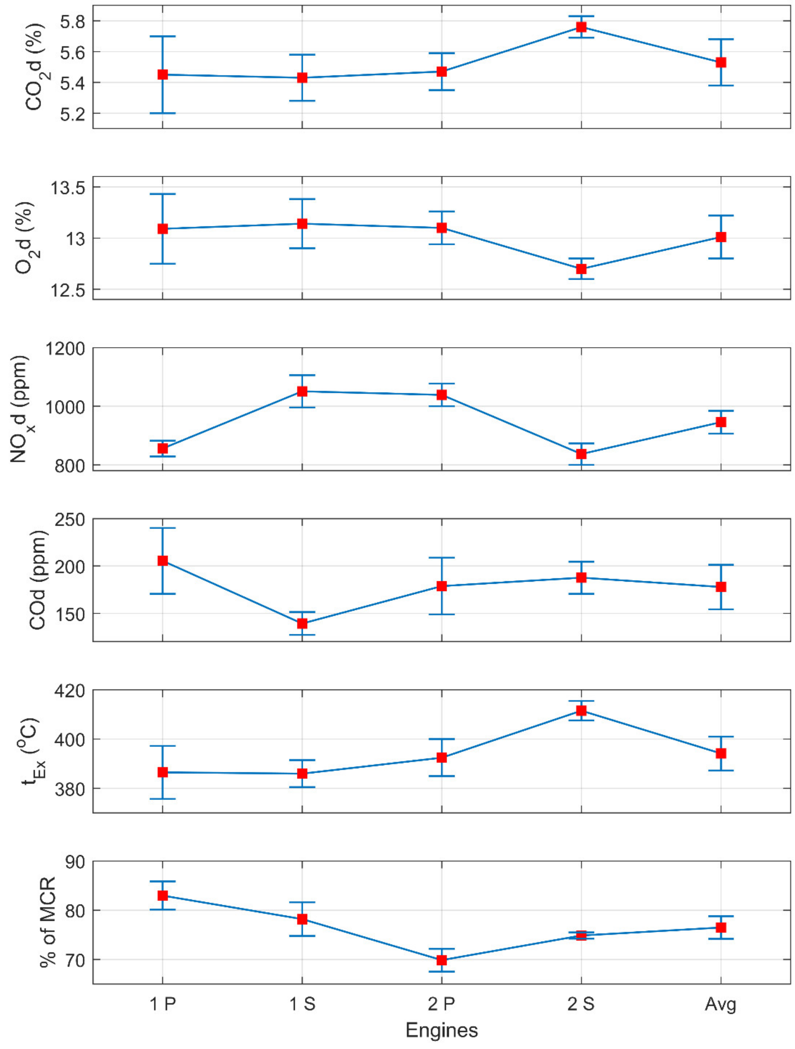
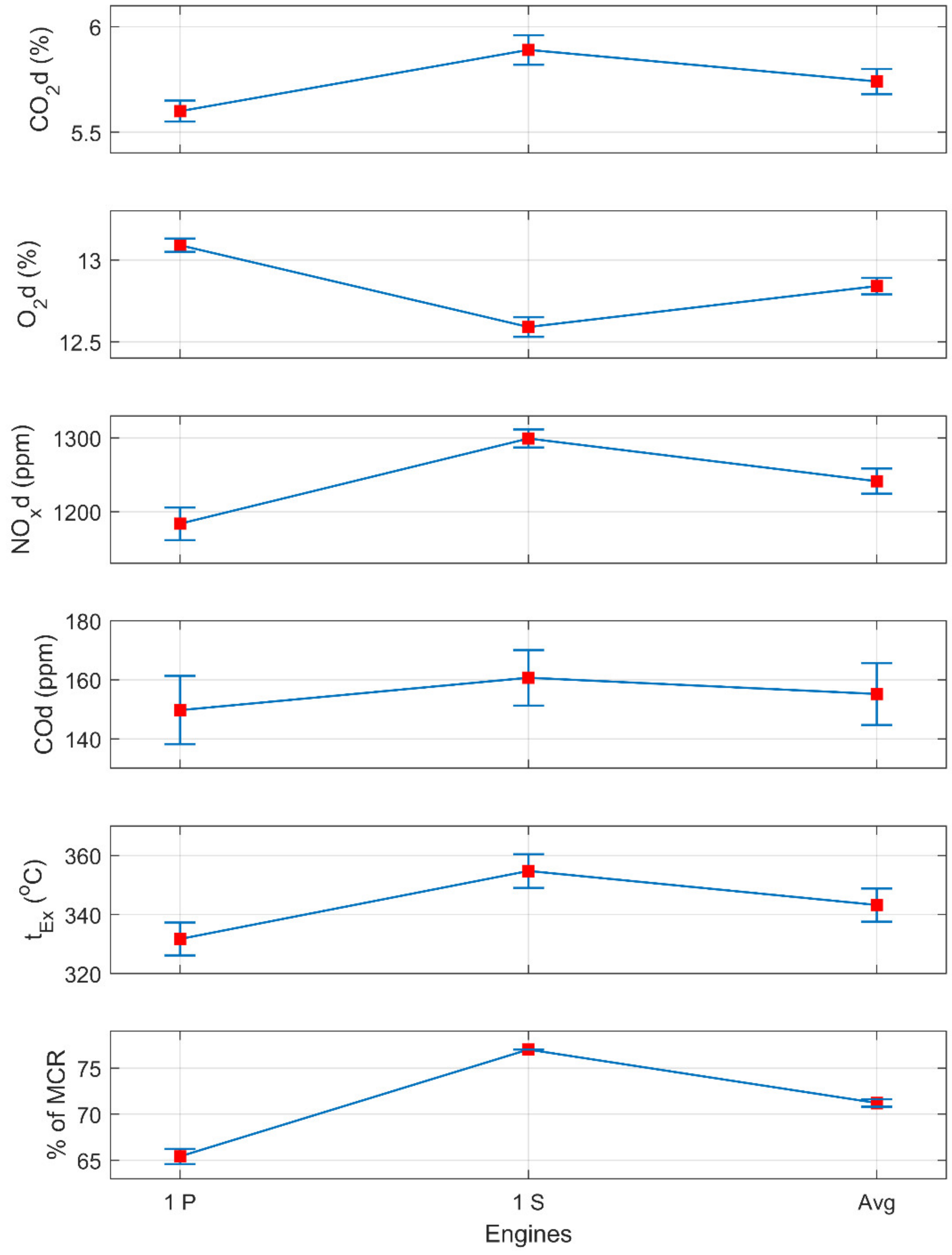
Figure 7, Figure 8 and Figure 9 show individual vessel and engine exhaust gas measurements and parameters with calculated average values. Red squared points show the mean value, and blue lines above and below the red points show the standard deviation of each measured or analysed value.
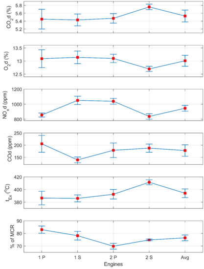
Figure 7.
Mean μ and standard deviation σ of measured and analysed parameters for Vessel 1 and its associated port (P) and starboard (S) engines with calculated average values.
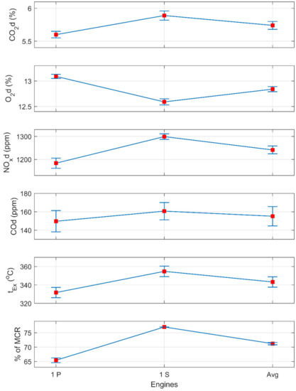
Figure 8.
Mean μ and standard deviation σ of measured and analysed parameters for Vessel 2 and its associated port (P) and starboard (S) engines with calculated average values.
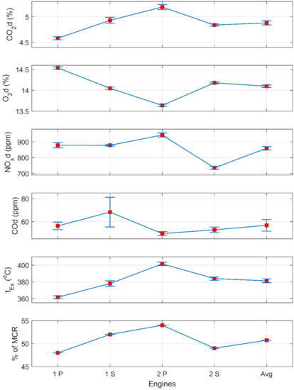
Figure 9.
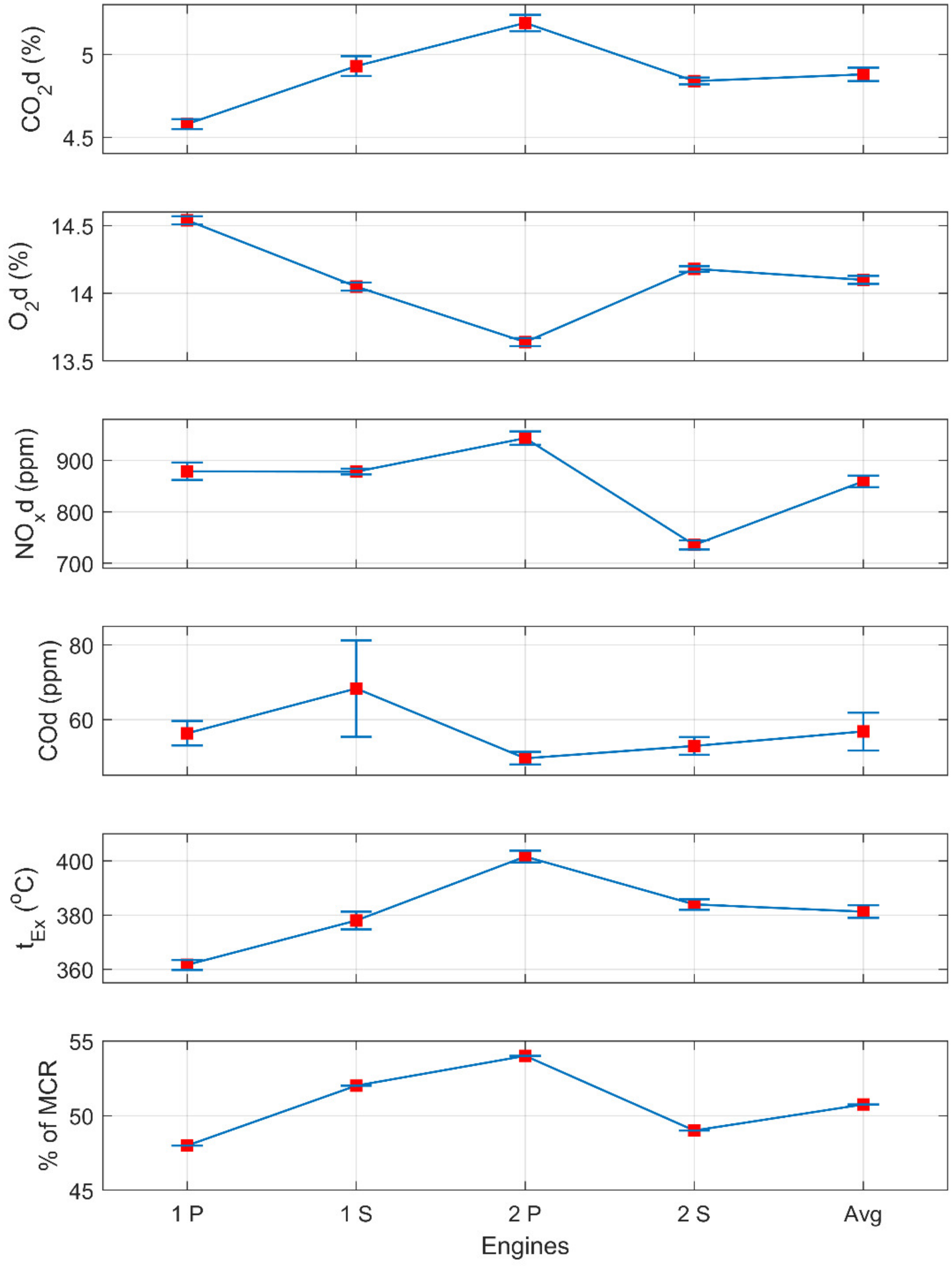
Mean μ and standard deviation σ of measured and analysed parameters for Vessel 3 and its associated port (P) and starboard (S) engines with calculated average values.
The simulators used for this research were Wärtsilä-Transas Marine NTPro 5000 navigational simulator and Wärtsilä ERS-LCHS 5000 TechSim engine room simulator [25,26]. The simulated vessel type was a Ro-Pax ferry with two main four-stroke engines each connected to its controllable pitch propeller via reduction gearbox, similar to Vessel 2 as shown in Figure 6. Other simulator vessel and engine particulars/parameters are provided in Table 1. Simulated Ro-Pax vessel was operated in a joint operation of the engine room and navigational simulators. This means that simulators are synchronously connected and operated as one vessel, which enables simultaneous recordings and later analysis of simulated vessel parameters, i.e., both from navigational and marine engine room point of view. The simulator was operated with various simulation scenarios of different weather and engine operating conditions typical for the Adriatic Sea [27] in order to record vessel and engine parameters. The simulator data obtained from these scenarios were partially used for the research published by Mannarini et al. [28] and were also used for this analysis in order to compare exhaust emissions from onboard measurements with simulated values.
The simulated vessel was operated with varying the wind speed from 0–34 m/s, significant wave height from 0–4 m, wind and wave relative direction to vessel heading from 0–180°, and engine telegraph lever position from 70–100, which corresponds to position 7–10 according to Figure 5. The total number of different simulation scenarios was 287 and each simulated scenario was recorded during the time frame of 25 min. Initial transient dynamics, during the first two minutes, were pruned and the remaining parameters were averaged although it should be noted that simulated signals behave as stationary ones with very low variance. The recorded simulator output variables presented in Table 3 were: engine shaft power as a percentage of maximum continuous rating (MCR) at which measurements were taken, concentration of CO2 as a percentage in a volume of dry exhaust gas, concentrations of NOx and CO in ppm in dry exhaust gas, exhaust gas temperature tEx after the turbocharger in °C, and specific fuel oil consumption (SFOC) in g/kWh. Values of oxygen O2 as a percentage in volume of dry exhaust gas and the amount of excess air λ could not be modelled/simulated so they were post-calculated. These values were calculated using the Equations (1)–(17) with the assumption that the used marine diesel oil has sulphur content in fuel less than 0.10% by mass, which is defined by EU directive 2016/802 for all EU ports and inland waters [21], and that emission conversion factor for marine diesel oil is 3.206 kg of CO2 in exhaust gases per 1 kg of burned marine diesel oil, which is defined by the International Maritime Organization (IMO) [29,30].
Table 3.
Simulated Ro-Pax vessel engine operating and exhaust gas simulated values.
4. Discussion
During the on board measurement process environmental loads, vessel speed and voyage duration influenced the engines shaft power/load. Engines shaft power proportionally changes with the change of the environmental loads and engine speed, as shown in Figure 4, and influence the exhaust gas measured parameters. Vessel 1 sailed under the longest averaged distances, had the highest averaged vessel speed and heaviest weather conditions when compared to other vessels. Vessel 2 and 3 sailed with similar averaged vessel speeds and weather conditions on voyages with similar averaged distances.
Data presented in Table 2 show that Vessel 1 sailed with the highest averaged engine shaft power (or load) on engines compared to other vessels. Averaged load on Vessel 1 engines was 76.48% and the lowest averaged engine load was 50.75% on Vessel 3. This higher load on Vessel 1 was caused due to the heavier weather and higher vessel speed due to the longer distances of the voyages. Averaged concentrations of CO2 and O2 in dry exhaust gases were similar on Vessel 1 and Vessel 2 which is normal due to almost similar engine loads. These engines were working with sufficient excess air quantity in order to enable complete combustion process in the cylinders and have a certain concentration of O2 in exhaust gases. Vessel 3 operated with lower CO2 and higher O2 concentrations in the dry exhaust gas, compared to the other vessels, which is typical for lower engine loads. The standard deviation for all averaged concentrations of CO2 and O2 in dry exhaust gases on all three vessels was very small. Highest averaged concentrations of CO in dry exhaust gases were on Vessel 1 because of the higher engine loads and engine speed, and the lowest on Vessel 3 for the opposite reasons. Highest averaged NOx concentrations were recorded on Vessel 2, and the lowest on Vessel 3. The formation of NOx concentration in exhaust gases is influenced with high combustion temperatures, pressures and the duration of the combustion process [31]. Engines on all three vessels were built before 1 January 2000 (Pre-2000 Engines), so the IMO emission standards, commonly referred to as Tier I, II and III standards, do not apply to these engines [32].
Figure 7 shows measured data and differences on all four main engines on Vessel 1. The standard deviation of all measured values is higher compared to other vessels because of the influence of heavier weather on main engines during the voyages. For Port engines (1 P and 2 P) and 1 Starboard (1 S) engine the averaged concentrations of CO2 and O2 in dry exhaust gases were similar except for the engine 2 Starboard (2 S) where concentrations of CO2 were higher and O2 lower. Additionally, for engine 2 S, averaged concentrations of NOx were the lowest, the exhaust gas temperatures after the turbocharger the highest and concentrations of CO the second highest. All of this can indicate the retarded injection timing or prolonged duration of the combustion process. Engine 1 S had the lowest averaged concentrations of CO, lowest exhaust gas temperatures and highest averaged concentrations of NOx, which can indicate the best combustion process among all engines. Higher NOx concentration, which results from higher combustion temperatures, should satisfy Tier I, II or III emission levels for engines built after the 1 January 2000.
Figure 8 shows measured data and differences on port and starboard main engines on Vessel 2. Starboard main engine had a higher averaged load than the port main engine and consequently higher exhaust gas temperatures after the turbocharger, higher averaged values of CO2 and NOx and slightly higher values of CO. Averaged concentrations of O2 in dry exhaust gases were lower on the port main engine compared to starboard engine. This data difference is normal for engines working at such different engine loads. Averaged concentrations of NOx on Vessel 2 are the highest when compared to other vessels which should be investigated further.
Figure 9 shows measured data and differences on all four main engines on Vessel 3. Main engine 2 Port (2 P) had the highest percentage of averaged load compared to other engines. That resulted with the highest averaged values of exhaust gas temperatures, concentrations of CO2, NOx and lowest values of averaged data for concentrations of O2 and CO in dry exhaust gases. All four engine data presented in Figure 8 follow the same line pattern as previously explained. As the averaged load increases the exhaust gas temperatures, averaged concentrations of CO2 and NOx increase (except for CO data for engine 2 P) and averaged data for concentrations of O2 and CO decrease (and vice versa).
Data presented in Table 3 show averaged simulator engine parameters during the engine shaft power/load change in percentage of MCR. Other values that are not provided by the simulator were post-calculated, as explained in the previous section. Engine loads, during simulation process, varied from 50–85%, which are usual loads on board vessels during the voyages and were also during the measurement processes. The data in the table can be divided in two parts, engine parameters lower and higher than 70% of MCR. The data in the table follow the previously mentioned pattern (with the minor exception at lower loads, at 60% and 67%). When the engine load increases, the exhaust gas temperatures, concentrations of CO2 and NOx increase and concentrations of O2 and CO decrease. At engine loads higher than 70% of MCR the turbocharger operates more efficiently and the exhaust gas temperature after the turbocharger decreases from 404 °C to 330 °C. This causes suction of more combustion air quantity into the cylinder (excess air λ is higher). As the engine load again increases (more than 72% of MCR), the simulated data follow the previously mentioned pattern.
In order to compare the on board measured values with simulated data, Table 4 was created. It shows a comparison of exhaust gas measurements and engine operating parameters from Vessel 1, Vessel 2 and simulated Ro-Pax vessel at the same loads. Vessel 1 engine data was compared with simulator data at 80% and 74% of MCR and Vessel 2 engine data was compared with simulator data at 67% and 77% of MCR. These were the cases during the measurement process where both controllable pitch propellers were connected to two main engines at specified engine load. Vessel 1 and 2 data for SFOC were taken from the engine instruction manuals [33,34] and excess air λ was calculated in the same manner as for the simulator data.
Table 4.
Comparison of exhaust gas measurements and engine operating parameters from Vessel 1, Vessel 2 and simulated Ro-Pax vessel.
At almost all compared engine loads the measured averaged concentrations of CO2 and O2 in dry exhaust gases were similar except for the Vessel 2/Engine Port when compared to simulated values. As explained earlier, this is because simulated engines’ turbocharger operates less efficiently at loads lower than 70% of MCR. This can be seen if the exhaust temperatures of simulated engines are observed. Only at 67% of MCR the exhaust temperature of simulated engines was higher than during the onboard measurements. Excess air λ depends on turbocharger efficiency and engine/turbocharging system design. The value of excess air directly influences on CO2 and O2 percentage in exhaust gases. Averaged concentrations of CO on simulated engines were lower than measured onboard vessels, which is normal for newer versions/designs of engines. Averaged concentrations of NOx were similar when comparing Vessel 1 and simulated engine. Vessel 2 had the highest averaged concentrations of NOx and for that reason fuel injection system/equipment on that vessel should be checked for proper operation. Equation (18) can be used for conversion from ppm to g/kWh of NOx for comparison with Tier I, II or III emission levels. All above mentioned differences between measured and simulated values can be even better explained when comparing SFOC data. Simulated engines have significantly lower specific fuel oil consumption when compared to Vessel 1 and 2 engines. Vessels 1 and 2 were built in 1973 and 1993, respectively, with much lower mean effective pressure (mep) inside the cylinders, lower engine speed and engine power (Table 1). Simulator engines are a replica of modern and efficient MAN B&W 8L32/40 type engine that enables operation in different load ranges with low fuel oil consumption. All other advantages of the latest type of this engine can be found in [35].
Ro-Pax vessels and simulated Ro-Pax vessel can be compared during one example voyage which duration is set to 8 h. The energy consumption is calculated according to:
where is the propulsion power [kW] generated with all active engines and is the voyage duration [h].
The propulsion power is calculated according to:
where is the number of engines that are used for propelling the vessel.
Fuel oil consumption could be then calculated according to the equation:
where is the specific fuel oil consumption .
For Vessel 1, with two main engines and engines load equal to 74% of MCR, the fuel oil consumption will be:
For simulated vessel, with two main engines and engines load equal to 74% of MCR, with the same energy consumption, the reduced voyage duration and reduced fuel oil consumption will be:
With the same voyage duration and energy consumption, reduced two engines load expressed as the % of MCR and fuel oil consumption will be:
The reduction of fuel oil consumption will be 1.11 tons or 1.02 tons per voyage. When multiplied with an emission factor of 3.206 kg of CO2 in exhaust gases per 1 kg of burned marine diesel oil it will be 3.56 tons of CO2 or 3.27 tons of CO2 less per voyage. A similar calculation can be done with other vessels parameters.
Presented results show that exhaust gas concentrations acquired during the on board measurements and from the simulation process, with the same engine loads, are similar and can be compared. Differences in excess air quantities and specific fuel oil consumption originate from differences in engine models and year of built. Newer engines have lower specific fuel oil consumptions which, as a result, will have reduced vessel’s fuel oil consumption and CO2 emission. Engine complete fuel oil combustion process and optimal point of operation are influenced by many parameters that could be used in different fuel efficiency and pollution minimization optimisation procedures.
In some cases, it is very difficult, expensive or impossible to measure on board exhaust gas emissions and also to acquire engine room and navigational simulators. Results show that exhaust gas data from one source can be used to validate the data from the other source in order to reduce the research expenses and help creating relevant emission database. Acquired data can be also used for creating exhaust gas emissions models, engine and vessel optimization models, ship routing models [36] and similar.
5. Conclusions
In this research, exhaust gas emissions were measured on three Ro-Pax vessels sailing in the Adriatic Sea. Testo 350 Maritime flue gas analyser was used for monitoring the concentrations of CO2 and O2 as a percentage in volume of dry exhaust gas, concentrations of CO and NOx in ppm in dry exhaust gas and exhaust gas temperature after the turbocharger. During the measurement of exhaust gases main engines on Ro-Pax vessels were operated at different averaged loads, from 48% to 83% of MCR. As the averaged load increases the exhaust gas temperatures, averaged concentrations of CO2 and NOx increase and averaged data for concentrations of O2 and CO decrease (and vice versa). Analysis and comparison of main engines concentrations of exhaust gases from the same vessel and other vessels can indicate possible inefficiencies/faults that are caused by incomplete combustion process which will increase fuel oil consumption. All 10 analysed main engines on three vessels had very good combustion process in the cylinders. On Vessel 1, one main engine had different exhaust gas values than other engines which can indicate small retarded injection timing or prolonged duration of the combustion process and both engines on Vessel 2 had higher NOx emissions, which should be further investigated. Averaged values from all 10 engines on three vessels were: 5.38% of CO2, 13.32% of O2, 1115 ppm of NOx and 130 ppm of CO in dry exhaust gas with the averaged exhaust gas temperature after the turbocharger of 373 °C at 66% of MCR.
For this research, Wartsila-Transas engine room and navigational simulators were also used for creating the additional database of the exhaust gases and engine operating parameters in different weather conditions typical for the Adriatic Sea. The recorded simulator output variables, which were similar to the on board measured parameters, were compared to the exhaust gas emissions and engine operating parameters of Vessels 1, 2 and 3 engines. Comparison of data measured on board vessels with simulated data showed that concentrations of exhaust gas components were similar for all engine loads and measured averaged concentrations. The difference in results was due to the difference in engine design parameters and year of built of analysed engines. Specific fuel oil consumption of simulated engines at analysed loads was 191–193 g/kWh, for Vessel 1 SFOC was 213–216 g/kWh and for Vessel 2 SFOC was 203–205 g/kWh. When comparing the simulated vessel with Vessel 1, for one voyage of 8 h, at engines load of 74% of MCR and with the same energy consumption, simulated vessel will arrive 30 min faster and consume 1.11 tons of fuel oil or will produce 3.56 tons of CO2 less per voyage. If the voyage is set for an equal duration of 8 h and with the same energy consumption, the simulated vessel engines load will be reduced to 69% of MCR and still consume 1.02 tons of fuel oil, i.e., it will produce 3.27 tons of CO2 less per voyage. Presented analysis shows that significant fuel oil and CO2 emission reduction per voyage could be accomplished by voyage and/or engine operation optimization. Finally, it should be noted that the values presented in Table 3 can be further used for any kind of future data-driven modelling with the purpose of exhaust gases estimation with respect to different engine operating conditions.
Research studies on exhaust gases on board Ro-Pax vessels are very limited so measured data presented in this research will help creating more relevant on board emission database and offer the possibility to enhance the estimation of emissions and comparison with the current emission database. Measured and simulated data can be used for root cause analysis, creating engine optimization and exhaust emissions models, ship routing models and similar. Results of this analysis could be of interest to shipowners, ship operators, environmentalists and all other in reducing the fuel oil consumption and emissions of greenhouse and harmful exhaust gases into the atmosphere.
The main limitations of the presented analysis and obtained results are naturally connected with a limited number of performed measurements and very bounded initial conditions, particularly in terms of a relatively small sample of various environmental conditions and sea states during the measurement campaign, as well as the selected vessels which are far away from being the state-of-the-art. However, these vessels still represent the majority of passenger ships in Adriatic and therefore the obtained results are also representative having that in mind. Nevertheless, the research results could be improved by enhancing the measurement procedures at different weather conditions and distances with the same vessels and on even more vessels, particularly the newer ones.
Author Contributions
Conceptualization, J.O., M.V. and V.K.; methodology, J.O. and M.V.; software J.O. and Z.P.; validation, J.O. and M.V.; formal analysis, J.O., M.V. and Z.P.; investigation, J.O., M.V., V.K. and Z.P.; resources, J.O. and M.V.; data curation, J.O., M.V. and Z.P.; writing—original draft preparation, J.O, M.V. and V.K.; writing—review and editing, J.O., M.V., V.K. and Z.P.; visualization, M.V., J.O. and V.K.; supervision, J.O. and M.V.; project administration, J.O.; funding acquisition, J.O. All authors have read and agreed to the published version of the manuscript.
Funding
This research was funded by the European Regional Development Fund through the Italy-Croatia Interreg programme, project GUTTA, grant number 10043587.
Institutional Review Board Statement
Not applicable.
Informed Consent Statement
Not applicable.
Data Availability Statement
The data presented in this study are available on request from the corresponding author.
Acknowledgments
This work was also supported by the Croatian Science Foundation under the project IP-2018-01-3739. The authors would like to extend their appreciations to the ship-owner office for all the help during the exploitation measurements.
Conflicts of Interest
The authors declare no conflict of interest. The funders had no role in the design of the study; in the collection, analyses, or interpretation of data; in the writing of the manuscript, or in the decision to publish the results.
References
- Regulation (EU) 2015/757 of the European Parliament and of the Council of 29 April 2015 on the Monitoring, Reporting and Verification of Carbon Dioxide Emissions from Maritime Transport, and Amending Directive 2009/16/EC (Text with EEA Relevance)—EUR-Lex. Available online: https://eur-lex.europa.eu/legal-content/EN/LSU/?uri=CELEX%3A32015R0757 (accessed on 16 March 2022).
- Reducing Emissions from the Shipping Sector. Available online: https://ec.europa.eu/clima/eu-action/transport-emissions/reducing-emissions-shipping-sector_en (accessed on 16 March 2022).
- Mannarini, G.; Carelli, L.; Salhi, A. EU-MRV: An Analysis of 2018’s Ro-Pax CO2 Data. In Proceedings of the 2020 21st IEEE International Conference on Mobile Data Management (MDM), Versailles, France, 30 June–3 July 2020; IEEE: Piscataway, NJ, USA, 2020; pp. 287–292. [Google Scholar]
- Data Collection System for Fuel Oil Consumption of Ships. Available online: https://www.imo.org/en/OurWork/Environment/Pages/Data-Collection-System.aspx (accessed on 16 March 2022).
- Cooper, D.A. Exhaust Emissions from High Speed Passenger Ferries. Atmos. Environ. 2001, 35, 4189–4200. [Google Scholar] [CrossRef]
- Bogdanowicz, A.; Kniaziewicz, T. Marine Diesel Engine Exhaust Emissions Measured in Ship’s Dynamic Operating Conditions. Sensors 2020, 20, 6589. [Google Scholar] [CrossRef]
- Jahangiri, S.; Nikolova, N.; Tenekedjiev, K. An Improved Emission Inventory Method for Estimating Engine Exhaust Emissions from Ships. Sustain. Environ. Res. 2018, 28, 374–381. [Google Scholar] [CrossRef]
- Jahangiri, S.; Nikolova, N.; Tenekedjiev, K. Empirical Testing of Inventories Applying On-Board Measurements of Exhaust Emissions at Port and at Sea. J. Sustain. Dev. Transp. Logist. 2018, 3, 6–33. [Google Scholar] [CrossRef]
- Khan, M.Y.; Ranganathan, S.; Agrawal, H.; Welch, W.A.; Laroo, C.; Miller, J.W.; Cocker, D.R. Measuring In-Use Ship Emissions with International and U.S. Federal Methods. J. Air Waste Manag. Assoc. 2013, 63, 284–291. [Google Scholar] [CrossRef] [PubMed] [Green Version]
- Agrawal, H.; Welch, W.A.; Henningsen, S.; Miller, J.W.; Cocker, D.R. Emissions from Main Propulsion Engine on Container Ship at Sea. J. Geophys. Res. 2010, 115, D23205. [Google Scholar] [CrossRef]
- Chu-Van, T.; Ristovski, Z.; Pourkhesalian, A.M.; Rainey, T.; Garaniya, V.; Abbassi, R.; Jahangiri, S.; Enshaei, H.; Kam, U.-S.; Kimball, R.; et al. On-Board Measurements of Particle and Gaseous Emissions from a Large Cargo Vessel at Different Operating Conditions. Environ. Pollut. 2018, 237, 832–841. [Google Scholar] [CrossRef] [PubMed] [Green Version]
- Agrawal, H.; Welch, W.A.; Miller, J.W.; Cocker, D.R. Emission Measurements from a Crude Oil Tanker at Sea. Environ. Sci. Technol. 2008, 42, 7098–7103. [Google Scholar] [CrossRef] [PubMed] [Green Version]
- Fu, M. Real-World Emissions of Inland Ships on the Grand Canal, China. Atmos. Environ. 2013, 81, 222–229. [Google Scholar] [CrossRef]
- Introduction to Fuel and Energy. Available online: http://eyrie.shef.ac.uk/eee/cpe630/comfun1.html (accessed on 17 March 2022).
- Trisha, S. How Much Air Is Required for Complete Combustion? In Thermodynamics; Engineering Notes India, 2018; Available online: https://www.engineeringenotes.com/thermal-engineering/fuels-and-combustion/how-much-air-is-required-for-complete-combustion-thermodynamics/51415 (accessed on 16 March 2022).
- Smith, C.B. (Ed.) 9—Management of Process Energy. In Energy, Management, Principles; Elsevier: Amsterdam, The Netherlands, 1981; pp. 236–279. ISBN 978-0-08-028036-3. [Google Scholar]
- Sarkar, D.K. (Ed.) Chapter 3—Fuels and Combustion. In Thermal Power Plant; Elsevier: Amsterdam, The Netherlands, 2015; pp. 91–137. ISBN 978-0-12-801575-9. [Google Scholar]
- Çengel, Y.A.; Boles, M.A. Thermodynamics: An Engineering Approach, 5th ed.; Tata McGraw-Hill: New York, NY, USA, 2006. [Google Scholar]
- Kosky, P.; Balmer, R.; Keat, W.; Wise, G. (Eds.) Chapter 7—Chemical Engineering. In Exploring Engineering, 5th ed.; Academic Press: Cambridge, MA, USA, 2021; pp. 129–145. ISBN 978-0-12-815073-3. [Google Scholar]
- ISO 8217 2017; Fuel Standard for Marine Distillate Fuels. ISO: Geneva, Switzerland, 2017.
- Directive (EU) 2016/802 of the European Parliament and of the Council of 11 May 2016 Relating to a Reduction in the Sulphur Content of Certain Liquid Fuels; 2016; Volume 132. Available online: https://eur-lex.europa.eu/legal-content/EN/TXT/PDF/?uri=CELEX:32016L0802&rid=5 (accessed on 17 March 2022).
- Available online: https://www.testo.com/hr-HR/testo-350-maritime/p/0563-3503 (accessed on 17 March 2022).
- Testo-350-Maritime-Instruction-Manual.pdf. Available online: https://static-int.testo.com/media/30/a7/476842882400/testo-350-maritime-Instruction-manual.pdf (accessed on 17 March 2022).
- Internal Company Document: Bunker Delivery Note; Croatiainspect: Zagreb, Croatia, 2019.
- Available online: https://www.wartsila.com/voyage/simulation-and-training/technological-simulators (accessed on 17 March 2022).
- Available online: https://www.wartsila.com/voyage/simulation-and-training/navigational-simulators (accessed on 17 March 2022).
- Farkas, A.; Parunov, J.; Katalinić, M. Wave statistics for the middle Adriatic Sea. Pomor. Zb. 2016, 52, 33–47. [Google Scholar] [CrossRef]
- Mannarini, G.; Carelli, L.; Orović, J.; Martinkus, C.P.; Coppini, G. Towards Least-CO2 Ferry Routes in the Adriatic Sea. J. Mar. Sci. Eng. 2021, 9, 115. [Google Scholar] [CrossRef]
- IMO. MEPC.1/Circ.684 Guidelines for Voluntary Use of the Ship Energy Efficiency Operational Indicator (EEOI); Technical Report; International Maritime Organization: London, UK, 2009.
- IMO: Fourth Greenhouse Gas Study. 2020. Available online: https://wwwcdn.imo.org/localresources/en/OurWork/Environment/Documents/Fourth%20IMO%20GHG%20Study%202020%20-%20Full%20report%20and%20annexes.pdf (accessed on 30 March 2022).
- European Maritime Safety Agency (EMSA): Possible Technical Modifications on Pre-2000 Marine Diesel Engines for NOx Reductions. 2008. Available online: http://www.emsa.europa.eu/tags/download/1017/604/23.html (accessed on 30 March 2022).
- US Environmental Protection Agency. Regulatory update—Overview of EPA’s Emission Standards for Marine Engines, August 2004; US Environmental Protection Agency: Washington, DC, USA, 2004.
- Internal Company Document: Instruction Manual for Stork Werkspoor Diesel 8TM410 Engine; Stork Werkspoor Diesel: Amsterdam, The Netherlands, 1972.
- Internal Company Document: Instruction Manual for Bazan MAN B&W 8L40/54 a Engine; Bazan Motores: Cartagena, Columbia, 1992.
- MAN B&W: L+V32/40 Project Guide—Marine Four-Stroke Diesel Engines Compliant with IMO Tier II. Available online: https://man-es.com/applications/projectguides/4stroke/manualcontent/L32-40_GenSet_TierII.pdf (accessed on 30 March 2022).
- Available online: https://www.gutta-visir.eu (accessed on 30 March 2022).


Publisher’s Note: MDPI stays neutral with regard to jurisdictional claims in published maps and institutional affiliations. |
© 2022 by the authors. Licensee MDPI, Basel, Switzerland. This article is an open access article distributed under the terms and conditions of the Creative Commons Attribution (CC BY) license (https://creativecommons.org/licenses/by/4.0/).