Article

Assessing Climate Change Trends and Their Relationships with Alpine Vegetation and Surface Water Dynamics in the Everest Region, Nepal

by
Mana Raj Rai
1,2,
Amnat Chidthaisong
1,2,*,
Chaiwat Ekkawatpanit
3 and
Pariwate Varnakovida
4
1
Joint Graduate School of Energy and Environment, King Mongkut’s University of Technology Thonburi, Bangkok 10140, Thailand
2
Center of Excellence on Energy Technology and Environment (CEE), PERDO, Ministry of Higher Education, Science, Research and Innovation, Bangkok 10140, Thailand
3
Civil Engineering Department, Faculty of Engineering, King Mongkut’s University of Technology Thonburi, Bangkok 10140, Thailand
4
Geospatial Engineering and Innovation Center, Faculty of Department of Mathematics, King Mongkut’s University of Technology Thonburi, Bangkok 10140, Thailand
*
Author to whom correspondence should be addressed.
Atmosphere 2021, 12(8), 987; https://doi.org/10.3390/atmos12080987
Submission received: 30 May 2021 / Revised: 27 July 2021 / Accepted: 28 July 2021 / Published: 31 July 2021
(This article belongs to the Section Climatology)

Abstract

:
The Himalayas, especially the Everest region, are highly sensitive to climate change. Although there are research works on this region related to cryospheric work, the ecological understandings of the alpine zone and climate impacts are limited. This study aimed to assess the changes in surface water including glacier lake and streamflow and the spatial and temporal changes in alpine vegetation and examine their relationships with climatic factors (temperature and precipitation) during 1995–2019 in the Everest region and the Dudh Koshi river basin. In this study, Landsat time-series data, European Commission’s Joint Research Center (JRC) surface water data, ECMWF Reanalysis 5th Generation (ERA5) reanalysis temperature data, and meteorological station data were used. It was found that the glacial lake area and volume are expanding at the rates of 0.0676 and 0.0198 km3/year, respectively; the average annual streamflow is decreasing at the rate of 2.73 m3/s/year. Similarly, the alpine vegetation greening as indicated by normalized difference vegetation index (NDVI) is increasing at the rate of 0.00352 units/year. On the other hand, the annual mean temperature shows an increasing trend of 0.0329 °C/year, and the annual precipitation also shows a significant negative monotonic trend. It was also found that annual NDVI is significantly correlated with annual temperature. Likewise, the glacial lake area expansion is strongly correlated with annual minimum temperature and annual precipitation. Overall, we found a significant alteration in the alpine ecosystem of the Everest region that could impact on the water–energy–food nexus of the Dudh Koshi river basin.

1. Introduction

Climate is a major driving factor for the distribution of the global forest ecosystem [1]. Climate, especially temperature and precipitation, varies along latitude and continental position [2]. Based on temperature and precipitation, the Köppen–Trewartha classification has divided global climate into six groups: tropical, dry climate, sub-tropical, temperate, boreal, and polar climate [3]. Besides this, altitude also creates a mountain system which is defined by a minimum elevation of 300 m and minimum slope of 2° over 25 km [4]. The mountain system contains distinct thermal belts, which are distinguished into a mountain (>15 °C), montane (6.4–10 °C), alpine (3.5–6.4 °C), and Nival belts (<3.5 °C) [5]. In the broader context, the mountain system can be grouped into three belts: montane belt, alpine belt, and Nival belt. Likewise, the mountain system of Nepal is also divided into six life zones according to altitude: tropical (<1000 m), subtropical (1000–2000 m), temperate (2000–3000 m), subalpine (3000–4000 m), alpine (4000–5000 m), and nival zone (>5000 m) [6].
The mountain system provides a wide array of ecosystem services. Around 20% (1.2 billion) of the world’s population resides in mountains areas and around half of humankind depends on mountain resources [7]. Mountains sustain the lowland river discharge with varying degrees through glacial melting. Besides this, the mountain system sustains plant life up to the alpine belt, termed as an alpine ecosystem and referred to the communities found above the tree-line elevation. The alpine ecosystem covers 3% of the global land area. Because the alpine ecosystem is limited by distinct climate factors, viz. low temperature, low rainfall, strong winds, high solar radiation, low atmospheric pressure, and short growing season, there are great concerns that climate change will adversely affect this as well as the whole mountain ecosystem.
The mountain system of Nepal has distinct characteristics where the variation of topography exists from lowland warm and humid subtropical climate to high altitude climate with freezing temperature [6]. The warm summer temperature in lowlands is around 22–27 °C, and there are high altitude regions with temperatures of 5–15 °C around Nepal. The precipitation of Nepal is dominated by the southeast tropical easterly monsoon from the Bay of Bengal. The Himalayas act as a cooling barrier which results in orographic precipitation in the summer season. The summer monsoon accounts for around 79.6% of the total precipitation of Nepal [8]. The winter monsoon of Nepal is associated with a sub-tropical westerly jet from the northeast direction and comprises around 3.5% of total precipitation. Consequently, the summer monsoon sustains the summer streamflow of Nepal, whereas the winter streamflow largely depends on snow and glacier melt [8]. Hence, temperature and precipitation are crucial for determining soil moisture, evaporation, streamflow, and snow cover. Besides this, the mountain system of Nepal comprises the world’s highest alpine ecosystem including the Everest region with elevation up to around 9 km above mean sea level. At present, the Everest region falls under Sagarmatha National Park. This region is recognized as the site of international importance (World Heritage Site, a conservation hotspot among WWF global 200 ecoregions, and a Ramsar site (Gokyo Lake)). The Everest region has an estimated 1074 species of flora and 247 species of fauna [9]. This region is the water source of the Dudh Koshi River that sustains 0.46 million people on the Dudh Koshi river basin [10]. In addition, the Dudh Koshi River possesses a hydropower potential of 2741.5 MW [11]. Consequently, the changes in temperature and precipitation upstream in the high elevation of the Everest region are linked with the livelihood of the Dudh Koshi river basin. Hence, the study of the highest alpine ecosystem is essential to analyze the existing situation and manage the future potential risk.
In recent decades, the climate change issue has been a widespread concern all around the globe [12]. A previous study indicated that Nepal Himalaya was experiencing high warming trend during 1935–1975 [13]. It is affirmed that alpine ecosystems are facing increasing warming and are greatly vulnerable to ongoing climate change as they are controlled by low temperatures [14]. Using a variety of tools and techniques including satellite-based NDVI, climate change and its impacts have been observed across the Himalayas of Asia [15,16,17,18]. These impacts include the expansion of alpine vegetation towards higher altitudes in Hindu Kush Himalaya [19] and the conversion of alpine meadows to shrublands in the Tibetan Plateau [20,21]. It is also reported that the shift in the alpine tree line is associated with a significant increase in air temperature in Western Himalayas, India [22]. However, there are results of studies showing different responses of vegetation to climate change, suggesting that these are site specific, and the responses are modified by local drivers. For example, a study of the Tibetan Plateau showed that temperature is rising, but the vegetation greening rate decreases along elevation gradients [16]. Similarly, a study of the entire Himalayas showed that most Himalaya regions show a greening trend, but, in the Eastern Himalayas, the vegetation shows a decreasing trend along with elevation [23]. Specific to the Nepal Himalaya, unfortunately, the analysis of vegetation dynamics in relation to changes in climate variables is still lacking.
Besides vegetation, climate warming has also been found to affect cryospheric processes (such as changes in snow cover and glacier permafrost) and related hydrological processes (such as water cycle and balance and river discharge) [7]. For example, globally, it was reported that during 1990–2018 the number and area of glacial lakes have rapidly increased from 9414 (5930 km2) to 14,394 (8950 km2), and the glacial lake volume has increased from 105.7 to 156.5 km3 [24]. Similarly, the increasing number and area of glacier lakes were also revealed in the central Himalayas region during 1990–2010 [25]. At the scale of Nepal Himalaya, the number and area of glacier lakes have increased from 606 (55.53 km2) to 1541 (80.95 km2) from 1977 to 2017 [26]. It was revealed that the glacier has retreated at the rate of 10–59 m/year in the Everest region [27]. The changes in the glacial lakes will favor vegetation growth by increasing the soil moisture and temperature. However, the glacial lakes at a higher altitude create a threat of glacial lake outburst flood (GLOF) to lowland people. Hence, the trend of glacial lake expansion by area and volume should be monitored on a long-term basis.
Although there are some studies on the vegetation dynamics Koshi river basin, and over Nepal, the study of high altitude forest ecosystem in response to climate change is still unexplored. This region has less human disturbance for land-use change because of extreme climate. Because of this, the alpine ecosystem is considered a quick indicator of the impacts of climate change. The long-term analysis of alpine vegetation of the Everest region will provide a better understanding of climate change interaction with high altitude. In addition, the trend analysis of the number and area of glacial lakes over a long-term basis is also new and useful for the prediction of water stress, adaptability, vulnerability, and overall water resource management in Nepal Himalaya. Specifically, to understand the relationships between climate variables and their potential impacts on the Everest region of Nepal, this study aimed to answer three research questions: (i) What are the trends of temperature and precipitation in the Everest region? (ii) What are the trends of glacial lake and streamflow changes in the Everest region? (iii) What are the NDVI trends and areal changes of alpine vegetation in the Everest region?

2. Materials and Methods

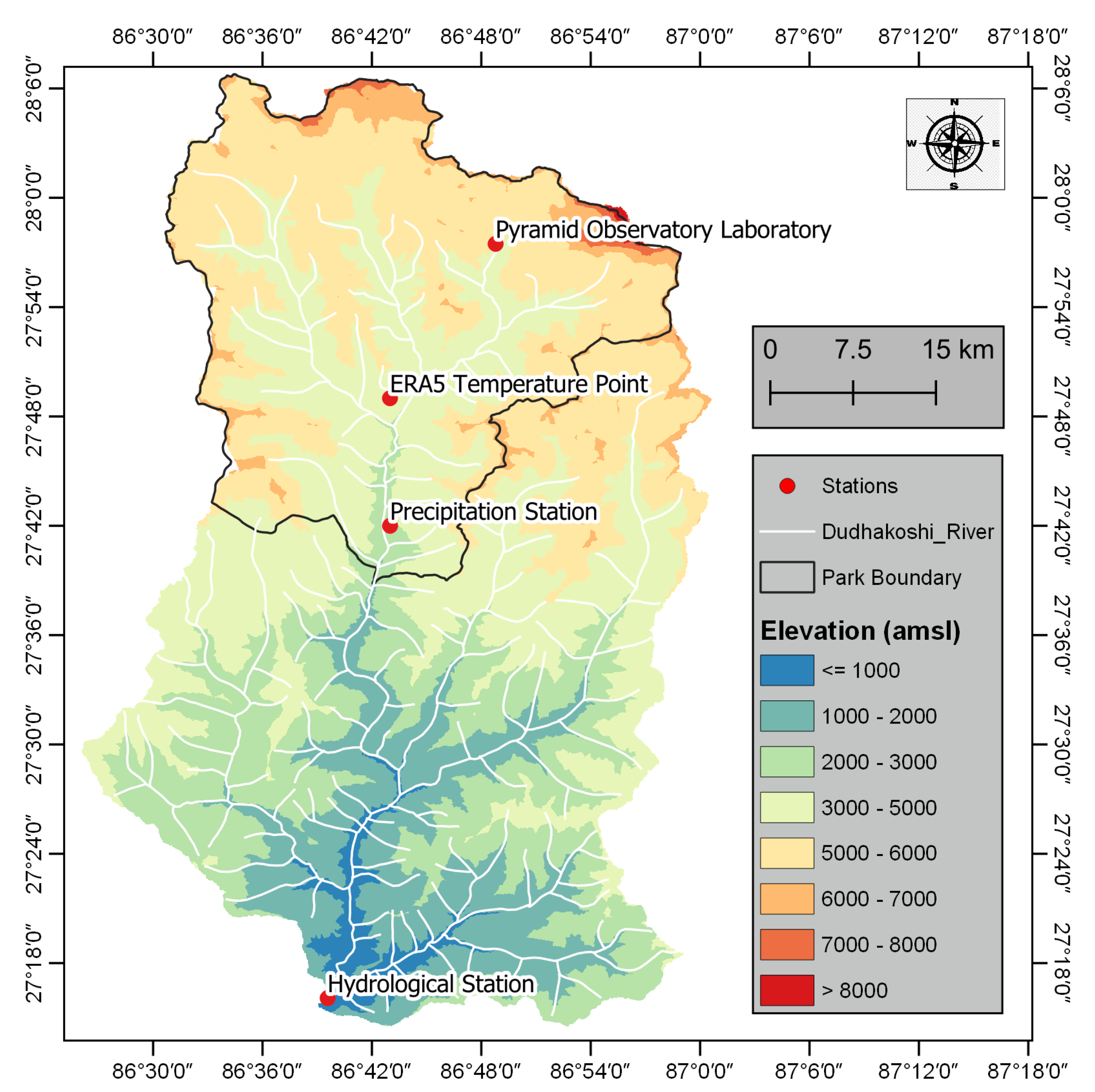
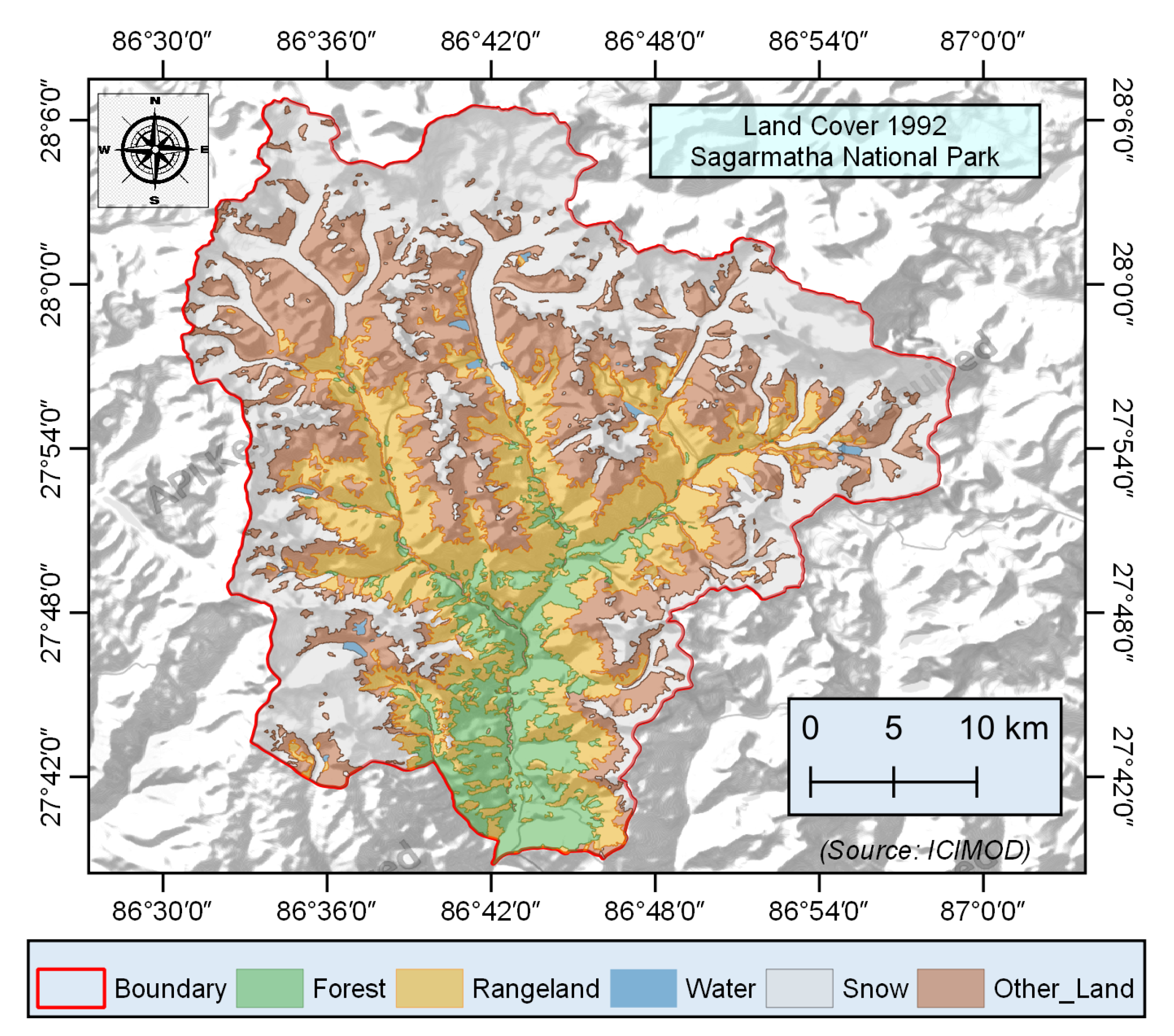
2.1. Site Description

This study focused on the high mountain system of Nepal in the Mount Everest region. This region is also designated as Sagarmatha National Park covering an area of 1413 km2. According to Garrard et al. (2016), regarding the land use/land cover of Sagarmatha National Park in 1992, bare rock/soil plus permanent ice covers 985.26 km2 (69.73% of total land area); rangeland, 301.49 km2 (21.34%); forest, 110.27 km2 (7.8%); agriculture and settlement, 10.21 km2 (0.72%); lake, 5.77 km2 (0.41%) [28]. According to another data source from ICIMOD (The International Center for Integrated Mountain Development, an intergovernmental institution for the study of Hindu Kush Himalaya), the land cover in 1992 of the Sagarmatha National Park comprised snow (590.38 km2), rangeland (301.84 km2), forest (120.29 km2), water (5.70 km2), and other lands (394.79 km2, Figure 1) (https://rds.icimod.org (accessed on 30 July 2021)).
Figure 2 shows the elevation zone of the study area covering the Dudh Koshi watershed area. This map was prepared based on the life zone of Nepal using QGIS software. Based on elevation, the study area can be divided into temperate (2845–3000 m), alpine (3000–5000 m), and nival zone (>5000 m). The alpine vegetation generally extends from 3000 to 5000 m in elevation. The streamflow is based on the accumulated flow from whole watershed areas of the Dudh Koshi river basin including the study area (Figure 2).

2.2. Climate Data

The basic technique to understand climate change is to analyze long-term records of climate variables from atmospheric observations. To check the seasonal variability, the annual climate is differentiated into four seasons: winter (December, January, and February; DJF), spring (March, April, and May; MAM), summer (June, July, and August; JJA), and autumn (September, October, and November; SON). However, the period of the season varies with continental position; thus, Nepal has adjusted the seasons into winter (DJF), spring (MAM), summer (JJAS), and autumn (ON), especially for precipitation and hydrological analysis [29].
In this study area, there is one climate station for observation of precipitation in Chaurikharka and one hydrological station on the downstream point of the Dudh Koshi watershed area at Rabuwa Bazar, operated by the Department of Hydrology and Meteorology (DHM), Nepal, as shown in Figure 2 [30]. However, the DHM does not have a temperature station in the vicinity of the Everest region. Alternatively, the temperature was analyzed by using ERA5 reanalysis data. The details of meteorological stations are listed in Table 1.
The handling of missing data is also important in the quality control of climate data. The threshold of omission of observation data for analysis seems different among the researchers. Zhai et al. (1999) omitted stations with more than 20 precipitation data missing in a year and 3 consecutive missing years or 5 randomly missing years [31]. Zubieta et al. selected a series with less than 5% missing data in a month [32]. Chapman and Walsh [33], Klein Tank et al. [34], and Haylock et al. [35] set a threshold of no more than 20% of missing daily, monthly, and annual data series, respectively. In this study, the proportions of monthly missing data in precipitation and streamflow were 1.35% and 5.56%, respectively.

2.2.1. Temperature

The ERA5 reanalysis temperature data (1995–2019) were extracted from Climate Data Store, Copernicus (https://cds.climate.copernicus.eu) (accessed date 30 July 2021), which have been produced by ECMWF/Copernicus Climate Change Service using R software. These reanalysis data are available on a regular latitude–longitude grid of 0.25° × 0.25° resolution, equivalent to approximately 31 km × 31 km, from 1950 to the present [36]. In this study, the ERA5 temperature data at Khumjung points were interpolated from gridded ERA5 data. ERA5 data are widely used to monitor climate change even inaccessible places and have been found effective and applicable [37,38]. Since reanalysis data are complete and consistent in time, missing data and outliers are not found in time-series data. After acquiring, the homogeneity of data was examined using the RHTests software package, which is based on penalized maximal F test [39]. The monthly data were converted into four seasonal series (winter (DJF), spring (MAM), summer (JJA), and autumn (SON)) and one annual series by the averaging method. The trend analysis of annual and seasonal time-series data was performed by using the modified Mann–Kendall test by the Hamed and Rao approach [40]. This non-parametric Mann–Kendall test has been used to evaluate the monotonic upward or downward trend of variables over time [41]. The Hamed and Rao approach has been used to address the autocorrelation in observed climate data [40]. Additionally, to determine the magnitude of change and forecasting, time-series data were also analyzed by linear regression test.
Reanalysis data are the best possible estimate and evenly spaced data grid of the current state of the Earth system using all available observations with a weather forecasting model. However, it is essential to validate with observation data to ensure their reliability. In this study, the ERA5 reanalysis data were compared with monthly data of 1995 (12 samples, 4% of population) of the nearest observation station, the Pyramid Observatory Laboratory (5050 m), which is located at 27.9592° N, 86.8131° E, Khumbu Glacier, in the Sagarmatha National Park, Nepal [42]. The independent t-test was used to compare the significance of the mean difference within two independent data.

2.2.2. Precipitation

Chaurikharka weather is the nearest permanent weather station, managed by DHM, Nepal. DHM is using a traditional US standard (8″ diameter) manual rain gauge to measure the rainfall form of precipitation [43]. For a better understanding of climate variation, climate observation stations should be placed at adequate spatial resolution. According to World Meteorological Organization (WMO), it is recommended that the spacing of climatological stations should not be more than 100 km [44]. The study area extends around 20 km east–west and 50 km north–south. Within this criterion, the Chaurikharka station is very likely to represent the study area.
The daily and monthly precipitation data (1995–2019) were obtained from DHM, Nepal. Then, collected data were scanned to detect outlier and missing data. The outlier data were sliced by the interquartile range (IQR) method. An outlier was sliced out when Xiq 50 > f × IQR; where Xi is ith observation, q50 is the 50th percentile, f is the multiplication factor (default f = 3), and IQR = q 75q 25 [45]. The proportion of missing data in the monthly series was found to be 1.35%. These missing monthly data were filled by the all-time (1995–2019) mean value of the corresponding month’s precipitation data. For example, a missing January datum was filled by the mean value of all January data from 1995 to 2019. After this, the homogeneity of data was examined using the RHTests software package. Thereafter, the monthly data were converted into four seasonal series (winter (DJF), spring (MAM), summer (JJAS), and autumn (ON)) by the summation method. The trend of seasonal and annual time-series data was analyzed by the modified Mann–Kendall test. Additionally, the linear regression test was used to evaluate the trendline of time-series data.

2.3. Surface Water

2.3.1. Glacial Lakes

The glacier lake area data (1995–2019) were extracted from JRC Global Surface Water Dataset, developed by The European Commission’s Joint Research Centre [46]. This dataset has already been validated using ground control points. The extent and change of water surface are provided at 30 m spatial resolution. The surface area of glacier lakes by month was computed and extracted using Google Earth Engine [47]. The data were further converted into seasonal and annual series by the averaging method. The trend analysis of surface area changes was performed by the modified Mann–Kendall test and linear regression test.
The volume of the glacier lake was determined using the area–volume empirical relationship developed by Huggel et al. [48] with the equation: V = 0.104 × A1.42, where V is the volume of glacier lake (m3) and A is the surface area of glacier lake (in m2). This relationship has been used and proved reasonable for the approximation of glacial lake volume.

2.3.2. Streamflow

The study area is the origin of the Dudh Koshi River, which drains from the Everest region. The snow and glacier melt of the Everest region contribute a significant portion of the streamflow of the Dudh Koshi River [49]. The streamflow has been monitored at Rabuwa Bazar gauging station and made available by DHM, Nepal. Although WMO has recommended 1000 km2 per station, this is the nearest available hydrological station representing the study area. In this study, the time-series data (1995–2015) were obtained from the records of the DHM. The outlier data were sliced by the IQR method. There were 5.56% of missing values in the monthly data. The monthly missing data were then replaced by the all-time (1995–2015) mean value of same month hydrological data. Thereafter, the homogeneity of data was examined using the RHTests software package. The monthly data were converted into four seasonal series (winter (DJF), spring (MAM), summer (JJAS), and autumn (ON)) and annual series by the averaging method. The seasonal and annual data from 2016 to 2019 were interpolated by a seasonal autoregressive integrated moving average (SARIMA) model. The model is written as SARIMA (p, d, q) × (P, D, Q, s), where p and seasonal P denote the number of time lags, d and seasonal D denote the degree of differencing, q and seasonal Q denote the number of moving average terms, and s denotes seasonal length in data [50]. The SARIMA (0, 1, 1) (0, 1, 1, 7) model was identified based on lowest Akaike information criterion (AIC) value, an estimation of prediction error. The trends of seasonal and annual time series were checked by the modified Mann–Kendall test and linear regression test.

2.4. Alpine Vegetation

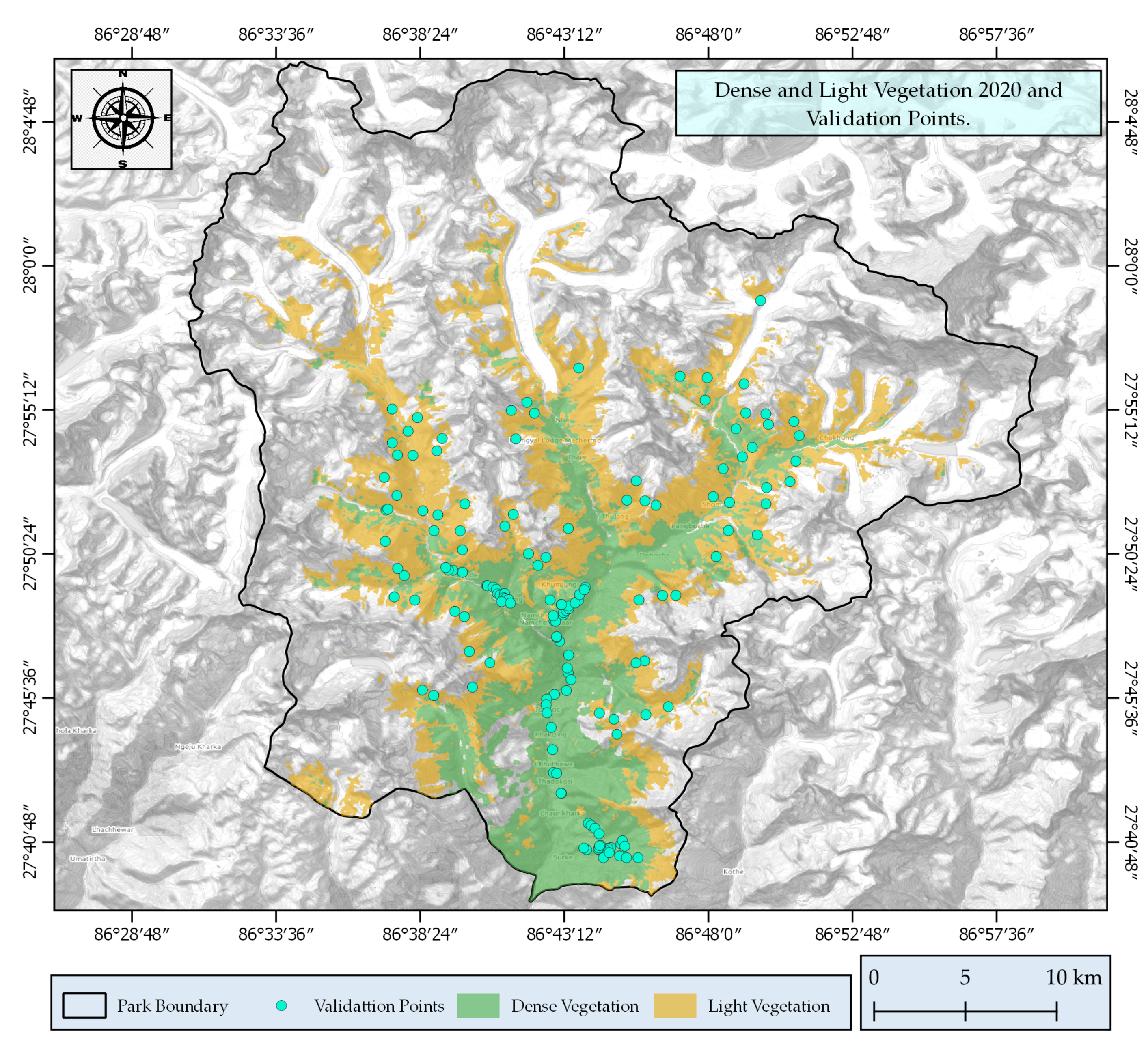
2.4.1. Spatial Change Detection

The spatial change detection of alpine vegetation (1995 and 2020) was based on satellite image analysis. Landsat Surface Reflectance Datasets by USGS were used for change detection of spatial extent. These datasets were processed and atmospherically corrected data, which are available in the Google Earth Engine (GEE) dataset. The satellite images for the autumn period (September to December) were used for vegetation analysis. In general, in the annual cycle of vegetation growth, spring (MAM) is the start of the growing season for grass, shrub, and trees; summer (JJA) is the major growing season; autumn (SON) is the start of leaf-falling for deciduous plants; winter (DJF) is the dormant season for plants. However, alpine vegetations are mostly perennial. Hence, the autumn season is assumed to be suitable for vegetation monitoring by satellite image analysis. Since the output was only targeted at vegetation, image classification was done by the NDVI thresholding method. NDVI is the most widely used index in vegetation analysis. This was computed as the difference between near-infrared (NIR) and red reflectance values divided by their sum. NDVI value ranges from −1 to +1. NDVI values between 0.2 and 0.5 were classified as light vegetation, while NDVI values between 0.5 and 1 were classified as dense vegetation. Light vegetation in the Everest region includes alpine meadows/rangeland and juniper scrubland. Dense vegetation includes conifer forest and birch–rhododendron forest. To validate the classified outputs, 75 points for dense vegetation and 75 points for light vegetation were created in QGIS software (Figure 3). Dense vegetation points were verified by ground observation, whereas light vegetation points were verified using Google Earth images. According to Congalton and Green (2019), the minimum number of sample points for accuracy assessment should be at least 20–100 points for each class [51].

2.4.2. NDVI Change Detection

USGS Landsat-5, -7, and -8 Tier 1 Surface Reflectance data were used for NDVI time-series analysis. NDVI data during 1995–2013 were acquired from Landsat-5 data, but there were no data in 2002 because of sensor error [52] and 2012 due to near failure of Landsat-5 [53]. Although Landsat-7 has data from 1999 to the present, the failure of Scan Line Corrector of ETM+ sensor results in a zigzag pattern of image and loss of 22–25% of data, and hence they have limited use in scientific research [53]. The NDVI data from 2013 to 2019 were therefore extracted from Landsat-8.
The image collection was filtered according to regions of interest (ROI), i.e., alpine zone and period (1995–2020). Regarding quality assurance, these products contain pixel quality attribute information. The cloud and cloud shadow pixels were masked out. The NDVI of each image was calculated, and the mean NDVI (>0.2) of ROI was computed and extracted in Google Earth Engine (GEE). The unavailable NDVI data for 2002 and 2012 were filled by the mean value of corresponding monthly NDVI data. Further, the monthly NDVI data were converted into seasonal and annual series by the averaging method. The trend analysis was also done by using Mann–Kendall test and linear regression test.

3. Results

3.1. Trends in Climate Variables

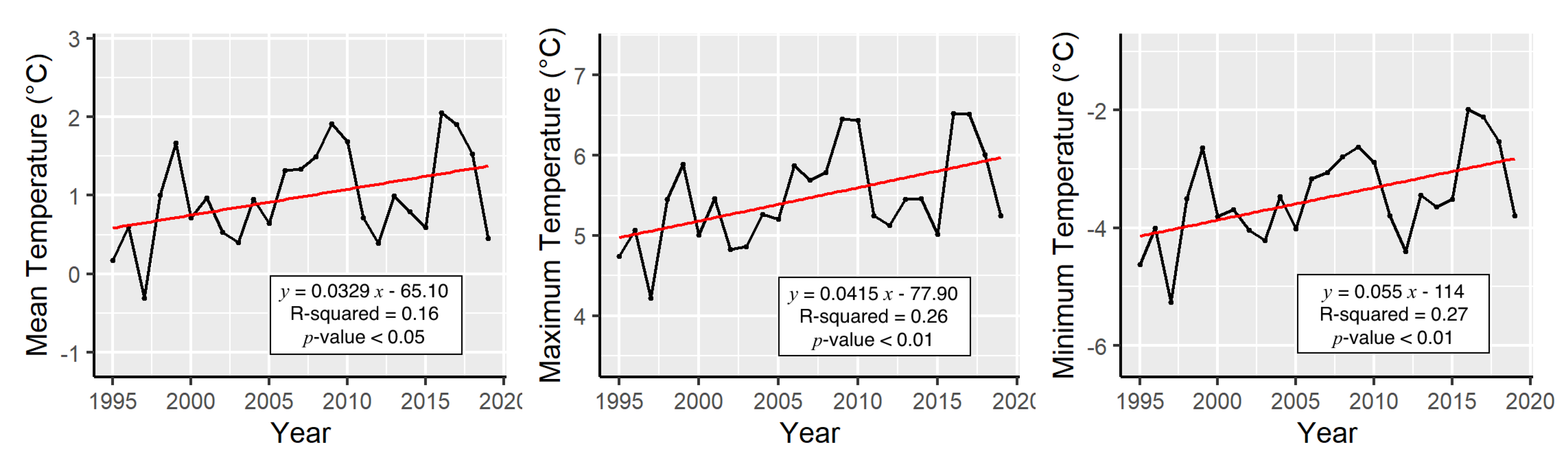
3.1.1. Temperature Trend

The results of the modified Mann–Kendall test for annual and seasonal temperature data for 1995–2019 are presented in Table 2. A positive z-value (Table 2) and slope value (Figure 4 and Table 3) indicate an increasing trend, whereas a negative z-value and slope value indicate a decreasing trend. The Kendall’s tau value explains the strength of correlation between variables, ranging from −1 to +1. Annual and seasonal temperature trends based on the linear regression method are shown in Figure 4 and Table 3. Significances are provided at 90%, 95%, and 99% confidence levels.
In Table 2, the maximum annual temperature and minimum annual temperature trends show the existence of a monotonic trend at a 95% confidence level. Similarly, the mean annual temperature also shows the existence of a monotonic trend at a 90% confidence level. Besides, all the positive tau values and z-values in Table 2 indicate that the temperature is positively correlated or increasing with time series. As shown in Figure 4, variations from years to years are common in temperature trends but all indicate the warming trends. The maximum and minimum annual temperature trends are increasing significantly at a 95% confidence level, whereas the mean annual temperature trend shows a significant positive trend at a 90% confidence level. Similarly, the significant increasing trend is shown in the summer season of mean, maximum, and minimum temperature at a 99% confidence level (Table 2). According to the linear regression test shown in Figure 4, the mean annual temperature, maximum annual temperature, and minimum annual temperature show significant increasing trends. The magnitude of trends for mean, maximum, and minimum annual temperatures are 0.0329, 0.0415, and 0.055 °C/year, respectively.
In addition, summer maximum temperature and summer minimum temperature show significant increasing trends of 0.0343 and 0.0341 °C/year, respectively. The winter maximum temperature and winter minimum temperature show higher significant increasing trends of 0.078 and 0.0915 °C/year, respectively. This shows that winter warming is around 2.5 times faster than summer warming. Similarly, an insignificant but coherent warming trend is also found in spring. Autumn maximum temperature and autumn minimum temperature show warming trends of 0.0358 and 0.0467 °C/year, respectively.
Since ERA5 reanalysis data are interpolated data, they were again compared with the nearest observation data by the independent t-test. The results are shown in Table 4. We found that there is no significant difference between the mean of reanalysis and observation data.

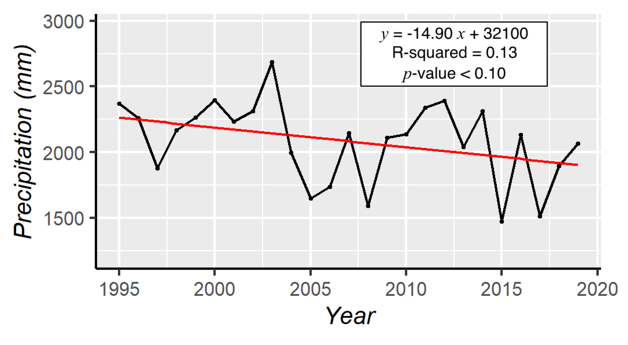
3.1.2. Precipitation Trend

As indicated in Table 5, the annual precipitation shows a decreasing monotonic trend at a 95% confidence level. Winter and autumn precipitation show the existence of a monotonic trend at a 95% confidence level. With a 90% confidence level, summer precipitation also shows a negative monotonic trend. The negative z-value and tau value indicate the decreasing trend. In Figure 5, a significantly decreasing trend with a 90% confidence level is observed in the annual precipitation series. The magnitude of the trend is −14.90 mm/year.

3.2. Surface Water

3.2.1. Glacial Lake Changes

The results of the modified Mann–Kendall test for annual and seasonal data are shown in Table 5. It is observed that the annual surface water extent in the Everest region shows a positive monotonic trend at a 95% confidence level.
The seasonal and annual surface water extent trends based on the linear regression test are shown in Table 3 and Figure 6a. We found that the surface area of glacial lakes is increasing at the rate of 0.068 km2/year. The significant increasing trend is shown at a 99% confidence level. Based on the season, winter and autumn seasons show an increasing rate of 0.078 and 0.15 km2/year, respectively (Table 3). The average surface area of glacier lakes in the study area is 4.9 km2. Thus, this observed increasing rate is quite significant. In Figure 6b, the glacial lake volume also shows a significant increasing trend with a rate of 0.0198 km3/year. The average glacial lake volume is 1.01 km3.

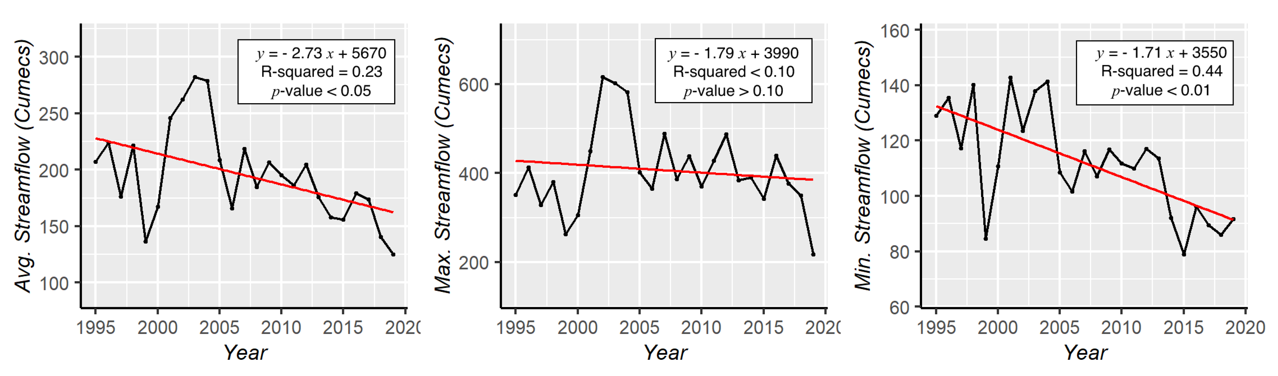
3.2.2. Streamflow Trend

According to the streamflow data for 1995–2015 recorded at Rabuwa Bazar gauging station, the maximum flowing rate is 2580 m3/s (cumecs), the minimum flowing rate is 9.07 m3/s, and the average flowing rate is 199 m3/s. The results of the modified Mann–Kendall test for annual and seasonal data are shown in Table 6 and Figure 7. In Table 6, it is observed that a significant decreasing trend is found in average annual streamflow and minimum annual streamflow at a 95% confidence level. The magnitudes of trend in average annual streamflow and minimum annual streamflow are −2.73 and −1.71 m3/s/year, respectively. It is also seen that the average summer streamflow and average minimum streamflow show significant decreasing trends. However, most of the trends for the maximum seasonal streamflow were not statistically significant. Similarly, all the spring season streamflows show significant decreasing trends.

3.3. Alpine Vegetation

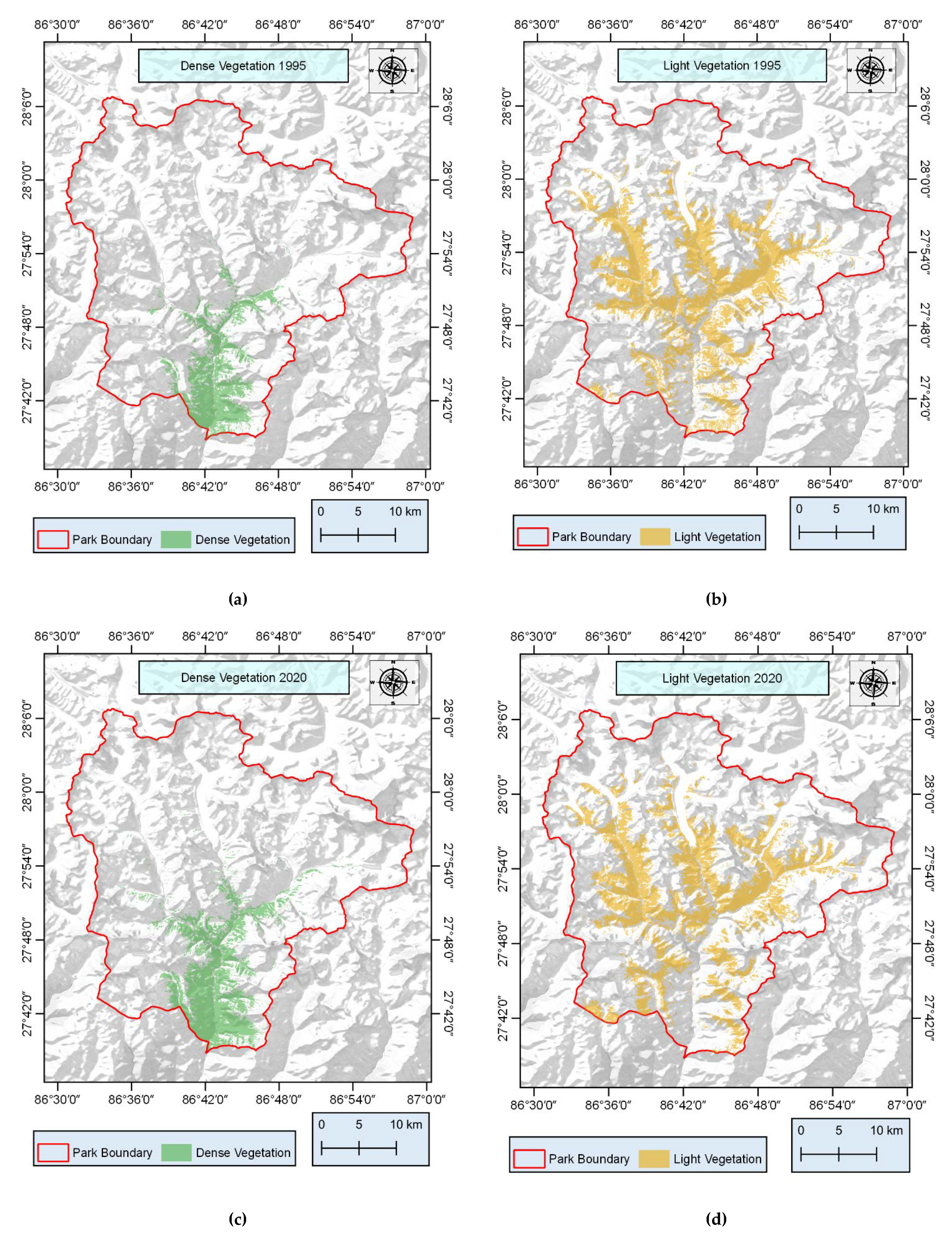
3.3.1. Spatial Change Detection

Alpine vegetation represents life at climate limits and is a quick indicator of climate change. Based on GIS analysis, around 97.5% of the study area is a high-altitude region having an elevation of more than 3000 m. Thus, alpine vegetation in the Everest region mostly possesses alpine grasses, juniper shrubs, and conifer forests. Figure 8 shows the vegetation maps in 1995 and 2020. It is observed that the dense vegetation increased from 103.5 to 150 km2 (45% increase), while light vegetation shows minor changes, increasing from 300.2 to 303.4 km2. This result shows the most marked expansion in dense vegetation in the Everest region. On the other hand, despite the constant areal extent, light vegetation such as alpine meadows/rangeland and juniper scrubs also shows expansion towards upper altitude, as shown in Figure 8.
To check the classification accuracy, 75 random sample points for dense vegetation were examined by field observation and 75 random sample points for light vegetation were examined by Google Earth imagery (Figure 3). Then, the confusion matrix was created, which showed that the overall classification accuracy is 76.33% for the classified image. The classification accuracy for the dense vegetation is 89%, whereas the classification accuracy of light vegetation is 72% (Table 7). The overall Kappa coefficient for 2020 is 0.76.

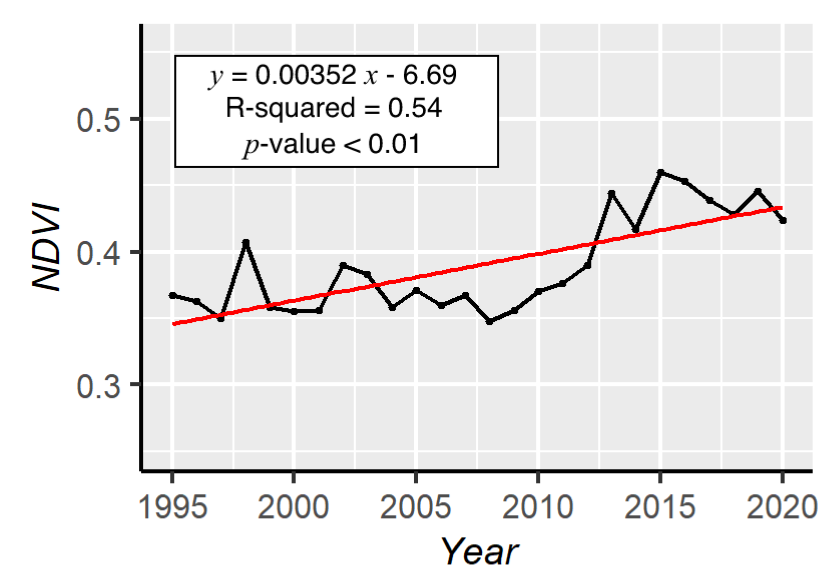
3.3.2. NDVI Change Detection

The result of the modified Mann–Kendall test for NDVI is shown in Table 5. It is revealed that there is a significant increasing trend in annual NDVI at a 95% confidence level. Similarly, all seasonal NDVI trends are also increasing significantly at a 95% confidence level.
Figure 9 and Table 3 show the linear regression trend of annual and seasonal NDVI during 1995–2019. It is noted that the NDVI is increasing at a rate of 0.0035 units/year. Seasonally, the autumn NDVI shows the highest increasing rate of 0.0051 units/year. More importantly, the spring growing season also shows a significant increasing trend. An abrupt rise in annual NDVI was observed in 2008. This also indicates the greening trend is increasing in the Everest region.

3.4. Alpine Region Change and Its Relationship with Climate Variables

The responses of alpine vegetation (NDVI) and surface water (glacial lake area plus streamflow) are analyzed by the multiple linear regression method (Table 8). Here, the temperature and precipitation variables are considered as independent (x) variables, while the NDVI, surface water, and streamflow are considered as dependent (y) variables.
The table shows that 65% of the annual variability of NDVI is explained by mean, maximum, and minimum annual temperature. Further, regarding the seasonal variability, autumn temperature and summer precipitation explain 94% of the variability of annual NDVI. Similarly, 71% variability of surface water extent is represented by minimum annual temperature and annual precipitation. Overall, there is a high level of confidence that alpine vegetation and temperature are strongly correlated.

4. Discussion

4.1. Climate Trend

Temperature, precipitation, and solar radiation are the major climate controls that act as limiting factors for vegetation growth [54]. Some studies found that temperature is responsible for 31–33% of Earth’s vegetation growth; precipitation is responsible for 40–52% of vegetation growth; solar radiation is responsible for 5–27% of vegetation growth [54,55]. In this study, it is revealed that the annual mean, maximum, and minimum temperatures at the Everest region are increasing at the rates of 0.0329, 0.0415, and 0.055 °C/year, respectively. In line with this result, Shrestha et al. [13] also found that the maximum temperature is increasing rate at 0.057 °C/year in the entire Nepal Himalayas. Within seasonal temperature, winter maximum temperature and winter minimum temperature show higher warming trends than the summer season. On the global scale, it is observed that winter warming is faster than summer warming [56]. Winter warming is ecologically more crucial. Winter warming can promote vegetation growth by reducing the seasonal frost of the winter season [57]. An experiment has discovered that soil respiration is increased by 9.3% by winter warming [58]. Winter warming stimulates litter decomposition in the winter season. Most importantly, prolonged winter warming triggers advancement in spring plant phenology and eventually increases the length of the growing season [59]. On the other hand, the annual precipitation of the Everest region shows a decreasing monotonic trend. However, the magnitude of change is found at −14.90 mm/year at a 90% confidence level. Besides this, summer precipitation also shows a decreasing trend at a 90% confidence level. Salerno et al. [60] also observed that the monsoon precipitation was weakening (−9.3 mm/year) in the Everest region during 1994–2013. Another larger-scale study including the Everest region by Shrestha et al. [61] found an increasing annual precipitation over the entire Koshi river basin (area of 87,970 km2) from 1975 to 2010. However, this study did not include the stations in the study area, and the results in this study might be due to local spatial variation. Hence, the climate condition of the Everest region has changed over the recent 25 years period. This climate change is very likely to alter the alpine ecosystem and cryospheric processes of the Everest region.

4.2. Surface Water Dynamics

It is estimated that the glaciers are decreasing an average of 267 Gt/year at the global scale and 6 Gt/year in South Asia [62]. As a result, glacial lakes are growing. In the Everest region, the result shows the increasing trend of glacial lake surface area at 0.0676 km2/year. The glacial lake volume has been increasing at the rate of 0.0198 km3/year. Bajracharya et al. [63] also found that the moraine-dammed lakes’ area, that is lakes formed due to blockade glacier debris, in the Dudh Koshi river basin increased from 2.291 to 7.254 km2 between 1996 and 2000. Similarly, Salerno et al. [64] found that the number and area of glacier lakes in the Everest region especially in the designated area of Sagarmatha National Park have increased. They reported 624 glacial lakes with an area of 7.43 km2 in 2008. The reason behind the glacial lake changes might be linked to temperature and precipitation change. A study of the Tibetan Plateau also found that the glacial lake expansion is highly correlated with glacier area recession, and this variation is associated with temperature rising [65]. The Everest region is also facing significant temperature rising, especially winter warming. Moreover, the glacial lake expansion may foster positive and negative impacts. There are unique glacier ecosystem services such as irrigation and drinking water supply to the downstream population and lowland discharge. However, most glacial lakes are formed by blockade of ice, glacier debris, landslide, and are inherently unstable type and susceptible to glacial lake outburst floods. Future endeavors should therefore be given to the study of glacial lake water resource utilization and their risk management.
Similarly, the average annual streamflow of the Dudh Koshi river basin is 199 m3/s. Dudh Koshi is a tributary of the Koshi River. The average flow of the Koshi River is 1658 m3/s. Similarly, the average flow of the three other major river basins of Nepal, namely, Gandaki, Karnali, and Mahakali, are 1753, 1441, and 698 m3/s, respectively [66]. In this study, from 1995 to 2019, we observed that the average annual streamflow is decreasing at the rate of 2.73 m3/s/year. These decreasing flow trends are consistent with weaker precipitation in the Everest region. Besides, the temperature is increasing, which might trigger more precipitation in the Everest region, but this is not the case. Gautam and Acharya [67] found a decreasing trend in the streamflow of the Dudh Koshi River basin from 1967 to 1997. Hence, the streamflow of the Dudh Koshi River is declining, which causes a water availability risk to the river-dependent ecosystems and societies. In addition to the need to closely monitor glacial lakes as mentioned above, it is also urgent and essential to evaluate the potential water stress associated with decreasing precipitation in this river basin.

4.3. Alpine Vegetation Dynamics

In this study, we found that NDVI is increasing at a rate of 0.00352 units annually. All the seasonal NDVIs are increasing with the highest in the autumn season. We also observed that annual NDVI is associated with autumn warming. Shi et al. found that autumn warning delays the end of the plant growing season for deciduous forests [68]. However, the study area consists of mostly evergreen conifer forests and perennial shrubs. Autumn warming also promotes vegetation growth by reducing frost damages [69]. The prominent increase in autumn NDVI reflects the increase in the extent of perennial vegetation. Additionally, the significant winter warming in the Everest region also favors vegetation growth. It is assessed that the dense vegetation cover has increased from 103.5 to 150 km2. Consistent with this, Baniya et al. [17] also observed a greening trend in all of Nepal with significant NDVI trends at 0.0005 and 0.002 units/year in the spring and autumn season, respectively. The driving factors for these increasing trends are attributed to temperature (39.62%), ecological restoration (25.16%), and multiple factors (35.22%). Over the larger scale in the Koshi river basin, Wu et al. [18] found a greening trend of 0.0023 units/year from 2000 to 2018. Zhang et al. [15] also showed the increasing rate of average growing season NDVI over the Koshi River basin at the rate of 0.0034 units/year from 2000 to 2011. In the context of greening in the Everest region, there might be multiple casual/control factors. The greening trend is increasing despite weaker precipitation. The ecological restoration program was also held in the study area. However, the area of the plantation during 1979–2008 is small (1.51 km2) as compared to the increasing area [9]. Ecological restoration in the Everest region is also challenging because of less water, cold weather, and rocky topography. Besides, the Everest region had around 1.02 km2 settlement area and 8.50 km2 agriculture area in 2011, and this region is managed under park regulations. Hence, the human disturbances to land-use change are considered minimal [28]. The shrub promotion due to overgrazing and abandonment of remote farmland is likely to favor vegetation expansion. Hence, it is obvious that the vegetation expansion is also driven by climatic factors. In this study, we found that annual NDVI is highly correlated with annual temperature. The abrupt rise of annual NDVI during 2008–2015 coincided with an increasing trendline in annual mean temperature during 2003–2009. Moreover, the annual precipitation showed an increasing trendline during 2008–2012 despite weak precipitation over the period. Furthermore, the temperature change can drive an upper shift in snow line altitude, which subsequently favors temperature for vegetation expansion and migration [70]. It is also revealed that temperature triggered alpine vegetation greening on the Tibetan Plateau from 1982 to 2011 [71]. For future endeavors, long-term research on phenological changes and carbon dynamics of the alpine vegetation may explore more about the climate change impacts on the high-altitude region.

5. Conclusions

This study demonstrates the changes in climate variables and their relationships with the change extents in surface water and alpine vegetation of the Everest region from 1995 to 2019. It is revealed that the mean, maximum, and minimum annual temperature increasing rates are 0.0329, 0.0415, and 0.055 °C/year, respectively. These increasing rates are statistically significant at a 95% confidence level. On the other hand, the annual precipitation also shows a significantly decreasing monotonic trend. The surface water area of glacial lakes shows an increasing rate of 0.0676 km2/year, whereas the glacial lake volume shows an increasing trend of 0.0198 km3/year. On the other hand, the average annual streamflow of the Dudh Koshi river basin is also decreasing at the rate of 2.73 m3/s/year. We also found that the alpine vegetation extent of the Everest region is changing. The dense vegetation cover in 2020 is 150 km2, a 46.5 km2 increase from the vegetation area in 1995. The greening trend in the Everest region is significant as the NDVI is increasing at a rate of 0.0035 units annually. In the context of seasonal variability, winter warming is 2.5 times faster than summer warming. The glacial lake change in the winter is increasing at the rate of 0.078 km2/year. The most prominent NDVI increase in the autumn season indicates vegetation expansion. Regarding the correlation of climate variables and NDVI, surface water extent, and streamflow, we found that annual NDVI is significantly correlated with maximum annual temperature, mean annual temperature, and minimum annual temperature. We also found that glacial lake expansion shows a significant association with minimum annual temperature and annual precipitation. Overall, this study reveals a significant alteration in the alpine ecosystem of the Everest region that could impact on the water–energy–food nexus of the Dudh Koshi river basin. The results indicate an urgent need for evaluation of the climate change impacts and implementation of effective planning to cope with threats from glacial melting and decreasing trends in precipitation, along with the expansion of alpine vegetation.

Author Contributions

Conceptualization, A.C.; methodology, M.R.R.; software, M.R.R.; formal analysis, M.R.R.; investigation, A.C., C.E. and P.V.; data curation, A.C.; writing—original draft preparation, M.R.R.; writing—review and editing, A.C., C.E. and P.V.; visualization, M.R.R.; supervision, A.C., C.E. and P.V. All authors have read and agreed to the published version of the manuscript.

Funding

The author has received a scholarship from the Thailand International Postgraduate Programme under TICA (No. 1604.2/3298) and financial support from the Joint Graduate School of Energy and Environment (JGSEE).

Data Availability Statement

The data presented in this study are available on request from the corresponding author.

Acknowledgments

The authors are grateful for the data providers USGS, GEE Platform, ECMWF, JRC, TMD, and DHM, Nepal. Special thanks are given to Chuman Thakur, a ranger at Sagarmatha National Park, Nepal for help in field data collection. Thanks are given to the Center for Climate Change Technology and Innovation, King Mongkut’s University of Technology Thonburi (KMUTT), Can Trong Nguyen, and Khun La Yaung for sharing knowledge on data analysis and support. We also thank the anonymous reviewers for providing valuable feedback and suggestions.

Conflicts of Interest

The authors declare no conflict of interest.

References

  1. Woodward, F.I.; Lomas, M.R.; Kelly, C.K. Global climate and the distribution of plant biomes. Philos. Trans. R. Soc. B Biol. Sci. 2004, 359, 1465–1476. [Google Scholar] [CrossRef] [PubMed] [Green Version]
  2. Bailey, R.G. Ecoregions: The Ecosystem Geography of the Oceans and Continents; Springer: New York, NY, USA, 2014; ISBN 9781493905232. [Google Scholar]
  3. Thornthwaite, C.W. An approach toward a rational classification of climate. Geogr. Rev. 1948, 38, 55–94. [Google Scholar] [CrossRef]
  4. Korner, C.; Ohsawa, M. Mountain systems. In Ecosystems and Human Well-Being: Current State and Trends; Island Press: Washington, DC, USA, 2005; Volume 1. [Google Scholar]
  5. Körner, C.; Paulsen, J.; Spehn, E.M. A definition of mountains and their bioclimatic belts for global comparisons of biodiversity data. Alp. Bot. 2011, 121, 73–78. [Google Scholar] [CrossRef] [Green Version]
  6. Government of Nepal Nepal Biodiversity Strategy. Available online: https://www.cbd.int/doc/world/np/np-nbsap-01-en.pdf (accessed on 30 July 2021).
  7. Viviroli, D.; Dürr, H.H.; Messerli, B.; Meybeck, M.; Weingartner, R. Mountains of the world, water towers for humanity: Typology, mapping, and global significance. Water Resour. Res. 2007, 43, 1–13. [Google Scholar] [CrossRef] [Green Version]
  8. PAN. Temporal and Spatial Variability of Climate Change over Nepal. Available online: https://www.dhm.gov.np/uploads/climatic/467608975Observed%20Climate%20Trend%20Analysis%20Report_2017_Final.pdf (accessed on 30 July 2021).
  9. ICIMOD/GoN. Nepal Biodiversity Resource Book: Protected Areas, Ramsar Sites, and World Heritage Sites. Available online: https://lib.icimod.org/record/7560 (accessed on 30 July 2021).
  10. Dixit, A.; Upadhya, M.; Dixit, K.; Pokhrel, A.; Rai, D.R. Living with Water Stress in the Hills of the Koshi Basin, Nepal. Available online: https://www.preventionweb.net/publications/view/12786 (accessed on 30 July 2021).
  11. Jha, R. Total run-of-river type hydropower potential of Nepal. Hydro Nepal J. Water Energy Environ. 2010, 7, 8–13. [Google Scholar] [CrossRef]
  12. Masson-Delmotte, V.; Zhai, P.; Pörtner, H.O.; Roberts, D.; Skea, J.; Shukla, P.R.; Pirani, A.; Moufouma-Okia, W.; Péan, C.; Pidcock, R. Global Warming of 1.5 °C. An IPCC Special Report on the Impacts of Global Warming of 1.5 °C above Pre-Industrial Levels and Related Global Greenhouse Gas Emission Pathways, in the Context of Strengthening the Global Response to the Threat of Climate Change. Available online: https://www.ipcc.ch/site/assets/uploads/sites/2/2019/06/SR15_Full_Report_High_Res.pdf (accessed on 30 July 2021).
  13. Shrestha, A.B.; Wake, C.P.; Mayewski, P.A.; Dibb, J.E. Maximum temperature trends in the Himalaya and its vicinity: An analysis based on temperature records from Nepal for the period 1971–1994. J. Clim. 1999, 12, 2775–2786. [Google Scholar] [CrossRef] [Green Version]
  14. Ernakovich, J.G.; Hopping, K.A.; Berdanier, A.B.; Simpson, R.T.; Kachergis, E.J.; Steltzer, H.; Wallenstein, M.D. Predicted responses of arctic and alpine ecosystems to altered seasonality under climate change. Glob. Chang. Biol. 2014, 20, 3256–3269. [Google Scholar] [CrossRef]
  15. Zhang, Y.; Gao, J.; Liu, L.; Wang, Z.; Ding, M.; Yang, X. NDVI-based vegetation changes and their responses to climate change from 1982 to 2011: A case study in the Koshi River Basin in the middle Himalayas. Glob. Planet. Chang. 2013, 108, 139–148. [Google Scholar] [CrossRef]
  16. Liu, L.; Wang, Y.; Wang, Z.; Li, D.; Zhang, Y.; Qin, D. Elevation-dependent decline in vegetation greening rate driven by increasing dryness based on three satellite NDVI datasets on the Tibetan Plateau. Ecol. Indic. 2019, 107, 105569. [Google Scholar] [CrossRef]
  17. Baniya, B.; Tang, Q.; Koirala, M.; Rijal, K.; Kattel, G. Growing season vegetation dynamics based on NDVI and the driving forces in Nepal during 1982–2015. For. J. Inst. For. Nepal 2020, 17, 1–22. [Google Scholar] [CrossRef]
  18. Wu, X.; Sun, X.; Wang, Z.; Zhang, Y.; Liu, Q.; Zhang, B.; Paudel, B.; Xie, F. Vegetation changes and their response to global change based on NDVI in the Koshi River Basin of central Himalayas since 2000. Sustainability 2020, 12, 6644. [Google Scholar] [CrossRef]
  19. Anderson, K.; Fawcett, D.; Cugulliere, A.; Benford, S.; Jones, D.; Leng, R. Vegetation expansion in the subnival Hindu Kush Himalaya. Glob. Chang. Biol. 2020, 26, 1608–1625. [Google Scholar] [CrossRef] [PubMed] [Green Version]
  20. Gao, Q.; Guo, Y.; Xu, H.; Ganjurjav, H.; Li, Y.; Wan, Y.; Qin, X.; Ma, X.; Liu, S. Climate change and its impacts on vegetation distribution and net primary productivity of the alpine ecosystem in the Qinghai-Tibetan Plateau. Sci. Total Environ. 2016, 554–555, 34–41. [Google Scholar] [CrossRef] [PubMed]
  21. Brandt, J.S.; Haynes, M.A.; Kuemmerle, T.; Waller, D.M.; Radeloff, V.C. Regime shift on the roof of the world: Alpine meadows converting to shrublands in the southern Himalayas. Biol. Conserv. 2013, 158, 116–127. [Google Scholar] [CrossRef]
  22. Mohapatra, J.; Singh, C.P.; Tripathi, O.P.; Pandya, H.A. Remote sensing of alpine treeline ecotone dynamics and phenology in Arunachal Pradesh Himalaya. Int. J. Remote Sens. 2019, 40, 7986–8009. [Google Scholar] [CrossRef]
  23. Mishra, N.B.; Mainali, K.P. Greening and browning of the Himalaya: Spatial patterns and the role of climatic change and human drivers. Sci. Total Environ. 2017, 587–588, 326–339. [Google Scholar] [CrossRef]
  24. Bokhorst, S.; Bjerke, J.W.; Melillo, J.; Callaghan, T.V.; Phoenix, G.K. Impacts of extreme winter warming events on litter decomposition in a sub-Arctic heathland. Soil Biol. Biochem. 2010, 42, 611–617. [Google Scholar] [CrossRef] [Green Version]
  25. Nie, Y.; Liu, Q.; Liu, S. Glacial lake expansion in the Central Himalayas by Landsat Images, 1990–2010. PLoS ONE 2013, 8, e83973. [Google Scholar] [CrossRef] [PubMed] [Green Version]
  26. Khadka, N.; Zhang, G.; Thakuri, S. Glacial lakes in the Nepal Himalaya: Inventory and decadal dynamics (1977–2017). Remote Sens. 2018, 10, 1913. [Google Scholar] [CrossRef] [Green Version]
  27. Bajracharya, S.R.; Mool, P. Glaciers, glacial lakes and glacial lake outburst floods in the Mount Everest region, Nepal. Ann. Glaciol. 2009, 50, 81–86. [Google Scholar] [CrossRef] [Green Version]
  28. Garrard, R.; Kohler, T.; Price, M.F.; Byers, A.C.; Sherpa, A.R.; Maharjan, G.R. Land use and land cover change in Sagarmatha National Park, a world heritage site in the Himalayas of Eastern Nepal. Mt. Res. Dev. 2016, 36, 299. [Google Scholar] [CrossRef]
  29. DHM. Observed Climate Trend Analysis in the Districts and Physiographic Regions of Nepal (1971–2014); Department of Hydrology and Meteorology: Kathmandu, Nepal, 2017. [Google Scholar]
  30. ICIMOD. Climatic and Hydrological Atlas of Nepal; International Centre for Integrated Mountain Development: Kathmandu, Nepal, 1996. [Google Scholar]
  31. Zhai, P.; Sun, A.; Ren, F.; Liu, X.; Gao, B.; Zhang, Q. Changes of climate extremes in China. Clim. Chang. 1999, 42, 203–218. [Google Scholar] [CrossRef]
  32. Zubieta, R.; Saavedra, M.; Silva, Y.; Giráldez, L. Spatial analysis and temporal trends of daily precipitation concentration in the mantaro river basin: Central Andes of Peru. Stoch. Environ. Res. Risk Assess. 2017, 31, 1305–1318. [Google Scholar] [CrossRef]
  33. Chapman, W.L.; Walsh, J.E. Recent variations of sea ice and air temperature in high latitudes. Am. Meteorol. Soc. 1993, 74, 33–47. [Google Scholar] [CrossRef] [Green Version]
  34. Klein Tank, A.M.G.; Wijngaard, J.B.; Können, G.P.; Böhm, R.; Demarée, G.; Gocheva, A.; Mileta, M.; Pashiardis, S.; Hejkrlik, L.; Kern-Hansen, C.; et al. Daily dataset of 20th-century surface air temperature and precipitation series for the European Climate Assessment. Int. J. Climatol. 2002, 22, 1441–1453. [Google Scholar] [CrossRef]
  35. Haylock, M.R.; Hofstra, N.; Klein Tank, A.M.G.; Klok, E.J.; Jones, P.D.; New, M. A European daily high-resolution gridded data set of surface temperature and precipitation for 1950–2006. J. Geophys. Res. 2008, 113, 1950–2006. [Google Scholar] [CrossRef] [Green Version]
  36. Hersbach, H.; Bell, B.; Berrisford, P.; Hirahara, S.; Horányi, A.; Muñoz-Sabater, J.; Nicolas, J.; Peubey, C.; Radu, R.; Schepers, D.; et al. The ERA5 global reanalysis. Q. J. R. Meteorol. Soc. 2020, 146, 1999–2049. [Google Scholar] [CrossRef]
  37. Zhu, J.; Xie, A.; Qin, X.; Wang, Y.; Xu, B.; Wang, Y. An assessment of ERA5 reanalysis for antarctic near-surface air temperature. Atmosphere 2021, 12, 217. [Google Scholar] [CrossRef]
  38. Jakovlev, A.R.; Smyshlyaev, S.P.; Galin, V.Y. Interannual variability and trends in sea surface temperature, lower and middle atmosphere temperature at different latitudes for 1980–2019. Atmosphere 2021, 12, 454. [Google Scholar] [CrossRef]
  39. Wang, X.L. Penalized maximal F test for detecting undocumented mean shift without trend change. J. Atmos. Ocean. Technol. 2008, 25, 368–384. [Google Scholar] [CrossRef]
  40. Hamed, K.H.; Rao, A.R. A modified Mann-Kendall trend test for autocorrelated data. J. Hydrol. 1998, 204, 182–196. [Google Scholar] [CrossRef]
  41. Mann, H.B. Non-parametric test against trend. Econometrica 1945, 13, 245–259. [Google Scholar] [CrossRef]
  42. Tartari, G.; Verza, G.; Bertolami, L. Meteorological data at the Pyramid Observatory Laboratory (Khumbu Valley, Sagarmatha National Park, Nepal). J. Limnol. 1998, 57, 23–40. [Google Scholar]
  43. Talchabhadel, R.; Karki, R.; Parajuli, B. Intercomparison of precipitation measured between automatic and manual precipitation gauge in Nepal. Measurement 2016, 106, 264–273. [Google Scholar] [CrossRef]
  44. WMO Guide to the Global Observing System: WMO-No 488; World Meteorological Organization: Geneva, Switzerland, 2017.
  45. Eischeid, J.K.; Bruce Baker, C.; Karl, T.R.; Diaz, H.F. The quality control of long-term climatological data using objective data analysis. J. Appl. Meteorol. 1995, 34, 2787–2795. [Google Scholar] [CrossRef] [Green Version]
  46. Pekel, J.F.; Cottam, A.; Gorelick, N.; Belward, A.S. High-resolution mapping of global surface water and its long-term changes. Nature 2016, 540, 418–422. [Google Scholar] [CrossRef] [PubMed]
  47. Gorelick, N.; Hancher, M.; Dixon, M.; Ilyushchenko, S.; Thau, D.; Moore, R. Google earth engine: Planetary-scale geospatial analysis for everyone. Remote Sens. Environ. 2017, 202, 18–27. [Google Scholar] [CrossRef]
  48. Huggel, C.; Kääb, A.; Haeberli, W.; Teysseire, P.; Paul, F. Remote sensing based assessment of hazards from glacier lake outbursts: A case study in the Swiss Alps. Can. Geotech. J. 2002, 39, 316–330. [Google Scholar] [CrossRef] [Green Version]
  49. Savéan, M.; Delclaux, F.; Chevallier, P.; Wagnon, P.; Gonga-Saholiariliva, N.; Sharma, R.; Neppel, L.; Arnaud, Y. Water budget on the Dudh Koshi River (Nepal): Uncertainties on precipitation. J. Hydrol. 2015, 531, 850–862. [Google Scholar] [CrossRef]
  50. Brockwell, P.J.; Davis, R.A. Introduction to Time Series and Forecasting; Springer: Berlin/Heidelberg, Germany, 2002; ISBN 9780387781884. [Google Scholar]
  51. Congalton, R.G.; Green, K. Assessing the Accuracy of Remotely Sensed Data: Principles and Practices; CRC Press: Boca Raton, FL, USA, 2019; ISBN 9781498776660. [Google Scholar]
  52. Storey, J.C.; Choate, M.J. Landsat-5 bumper-mode geometric correction. IEEE Trans. Geosci. Remote Sens. 2004, 42, 2695–2703. [Google Scholar] [CrossRef]
  53. Markham, B.L.; Storey, J.C.; Williams, D.L.; Irons, J.R. Landsat sensor performance: History and current status. IEEE Trans. Geosci. Remote Sens. 2004, 42, 2691–2694. [Google Scholar] [CrossRef]
  54. Churkina, G.; Running, S.W. Contrasting climatic controls on the estimated productivity of global terrestrial biomes. Ecosystems 1998, 1, 206–215. [Google Scholar] [CrossRef]
  55. Nemani, R.R.; Keeling, C.D.; Hashimoto, H.; Jolly, W.M.; Piper, S.C.; Tucker, C.J.; Myneni, R.B.; Running, S.W. Climate-driven increases in global terrestrial net primary production from 1982 to 1999. Science 2003, 300, 1560–1563. [Google Scholar] [CrossRef] [PubMed] [Green Version]
  56. Balling, R.C.; Michaels, P.J.; Knappenberger, P.C. Analysis of winter and summer warming rates in gridded temperature time series. Clim. Res. 1998, 9, 175–181. [Google Scholar] [CrossRef] [Green Version]
  57. Schuerings, J.; Beierkuhnlein, C.; Grant, K.; Jentsch, A.; Malyshev, A.; Peñuelas, J.; Sardans, J.; Kreyling, J. Absence of soil frost affects plant-soil interactions in temperate grasslands. Plant. Soil 2013, 371, 559–572. [Google Scholar] [CrossRef]
  58. Kreyling, J.; Grant, K.; Hammerl, V.; Arfin-Khan, M.A.S.; Malyshev, A.V.; Peñuelas, J.; Pritsch, K.; Sardans, J.; Schloter, M.; Schuerings, J.; et al. Winter warming is ecologically more relevant than summer warming in a cool-temperate grassland. Sci. Rep. 2019, 9, 14632. [Google Scholar] [CrossRef] [Green Version]
  59. Parmesan, C.; Yohe, G. A globally coherent fingerprint of climate change impacts across natural systems. Nature 2003, 421, 37–42. [Google Scholar] [CrossRef]
  60. Salerno, F.; Guyennon, N.; Thakuri, S.; Viviano, G.; Romano, E.; Vuillermoz, E.; Cristofanelli, P.; Stocchi, P.; Agrillo, G.; Ma, Y.; et al. Weak precipitation, warm winters and springs impact glaciers of south slopes of Mt. Everest (central Himalaya) in the last 2 decades (1994–2013). Cryosphere 2015, 9, 1229–1247. [Google Scholar] [CrossRef] [Green Version]
  61. Shrestha, A.B.; Bajracharya, S.R.; Sharma, A.R.; Duo, C.; Kulkarni, A. Observed trends and changes in daily temperature and precipitation extremes over the Koshi river basin 1975–2010. Int. J. Climatol. 2017, 37, 1066–1083. [Google Scholar] [CrossRef] [Green Version]
  62. Zemp, M.; Huss, M.; Thibert, E.; Eckert, N.; McNabb, R.; Huber, J.; Barandun, M.; Machguth, H.; Nussbaumer, S.U.; Gärtner-Roer, I.; et al. Global glacier mass changes and their contributions to sea-level rise from 1961 to 2016. Nature 2019, 568, 382–386. [Google Scholar] [CrossRef]
  63. Bajracharya, S.R.; Mool, P.K.; Shrestha, B.R. Impact of Climate Change on Himalayan Glaciers and Glacial Lakes: Case Studies on GLOF and Associated Hazards in Nepal and Bhutan; International Centre for Integrated Mountain Development (ICIMOD): Kathmandu, Nepal; United Nations Environment Programme (UNEP): Nairobi, Kenya, 2007. [Google Scholar]
  64. Salerno, F.; Thakuri, S.; D’Agata, C.; Smiraglia, C.; Manfredi, E.C.; Viviano, G.; Tartari, G. Glacial lake distribution in the Mount Everest region: Uncertainty of measurement and conditions of formation. Glob. Planet. Chang. 2012, 92–93, 30–39. [Google Scholar] [CrossRef]
  65. Wang, X.; Siegert, F.; Zhou, A.G.; Franke, J. Glacier and glacial lake changes and their relationship in the context of climate change, Central Tibetan Plateau 1972–2010. Glob. Planet. Chang. 2013, 111, 246–257. [Google Scholar] [CrossRef]
  66. Water and Energy Commission Secretariat. Water Resources of Nepal in the Context of Climate Change; Water and Energy Commission Secretariat: Kathmandu, Nepal, 2011. [Google Scholar]
  67. Gautam, M.R.; Acharya, K. Streamflow trends in Nepal. Hydrol. Sci. J. 2012, 57, 344–357. [Google Scholar] [CrossRef]
  68. Shi, C.; Sun, G.; Zhang, H.; Xiao, B.; Ze, B.; Zhang, N.; Wu, N. Effects of warming on chlorophyll degradation and carbohydrate accumulation of alpine herbaceous species during plant senescence on the tibetan plateau. PLoS ONE 2014, 9, e107874. [Google Scholar] [CrossRef] [PubMed]
  69. Li, P.; Zhu, Q.; Peng, C.; Zhang, J.; Wang, M.; Zhang, J.; Ding, J.; Zhou, X. Change in Autumn Vegetation Phenology and the Climate Controls From 1982 to 2012 on the Qinghai–Tibet Plateau. Front. Plant. Sci. 2020, 10, 1677. [Google Scholar] [CrossRef] [PubMed] [Green Version]
  70. Pandey, P.; Kulkarni, A.V.; Venkataraman, G. Remote sensing study of snowline altitude at the end of melting season, Chandra-Bhaga basin, Himachal Pradesh, 1980–2007. Geocarto Int. 2013, 28, 311–322. [Google Scholar] [CrossRef]
  71. Chen, X.; An, S.; Inouye, D.W.; Schwartz, M.D. Temperature and snowfall trigger alpine vegetation green-up on the world’s roof. Glob. Chang. Biol. 2015, 21, 3635–3646. [Google Scholar] [CrossRef]
Figure 1. Land cover map of the study area (Sagarmatha National Park).
Atmosphere 12 00987 g001
Figure 2. The elevation zone of the study area covering the Dudh Koshi watershed area.
Atmosphere 12 00987 g002
Figure 3. Validation points for dense vegetation and light vegetation for 2020.
Atmosphere 12 00987 g003
Figure 4. Linear regression trends of annual temperatures.
Atmosphere 12 00987 g004
Figure 5. Linear regression trends of annual precipitation.
Atmosphere 12 00987 g005
Figure 6. Glacial lake: (a) change in surface area; (b) changes in lake volume.
Atmosphere 12 00987 g006
Figure 7. Linear regression trends of annual streamflow.
Atmosphere 12 00987 g007
Figure 8. Alpine vegetation: (a) dense vegetation in 1995; (b) light vegetation 1995; (c) dense vegetation in 2020; (d) light vegetation in 2020.
Atmosphere 12 00987 g008
Figure 9. Linear regression trends of NDVI.
Atmosphere 12 00987 g009
Table 1. Detailed information on climate stations used in this study.
Station IDStation/Site NameTypeLatitudeLongitudeElevation (m)Start YearEnd Year
1202ChaurikharkaPrecipitation27° 42′ 00″86° 43′ 00″26191 January 199531 December 2019
670Rabuwa BazarDischarge27° 16′ 00″86° 39′ 35″4601 January 199512 December 2015
-KhumjungTemperature27° 49′ 00″86° 43′ 00″38001 January 199512 December 2019
Table 2. Summary of the modified Mann–Kendall statistical tests of temperature trend.
SeriesMean TemperatureMaximum TemperatureMinimum Temperature
z-ValueTaupz-ValueTaupz-ValueTaup
Winter1.910.200.061.660.240.103.180.29<0.01
Spring0.540.080.591.080.160.281.910.270.06
Summer3.790.54<0.013.290.47<0.013.120.45<0.01
Autumn1.130.180.261.970.280.051.410.220.16
Annual1.780.260.072.270.330.022.460.350.01
Table 3. Linear regression equations of all seasonal series of temperature, precipitation, streamflow, NDVI, and surface water area.
Climate VariablesSeason Variables (y)Regression LineR2p-Value
Mean TemperatureWintery = 0.0579x − 123R2 = 0.08ns
Springy = 0.0178x − 35.60R2 = 0.02ns
Summery = 0.0287x − 49.40R2 = 0.46***
Autumny = 0.0279x − 53.60R2 = 0.09ns
Maximum TemperatureWintery = 0.078x − 157R2 = 0.13*
Springy = 0.0181x − 31.50R2 = 0.02ns
Summery = 0.0343x − 57.80R2 = 0.40***
Autumny = 0.0358x − 65R2 = 0.17**
Minimum TemperatureWintery = 0.0915x − 196R2 = 0.14*
Springy = 0.0482x − 102R2 = 0.10ns
Summery = 0.0341x − 62.90R2 = 0.38***
Autumny = 0.0467x − 95.50R2 = 0.14*
PrecipitationWintery = −1.49x + 3030R2 = 0.06ns
Springy = 0.973x − 1750R2 = 0.02ns
Summery = −12x + 25,800R2 = 0.09ns
Autumny = −2.46x + 4990R2 = 0.11ns
Average StreamflowWintery = 0.29x − 534R2 = 0.09ns
Springy = −2.64x + 5440R2 = 0.22**
Summery = −11.4x + 23,400R2 = 0.34***
Autumny = −2.48x + 5110R2 = 0.35***
Maximum StreamflowWintery = 0.0713x − 87.60R2 ≤ 0.01ns
Springy = −1.07x + 2230R2 = 0.10ns
Summery = 1.05x − 1080R2 ≤ 0.01ns
Autumny = −2.19x + 4630R2 = 0.02ns
Minimum StreamflowWintery = 0.0779x − 115R2 = 0.01ns
Autumny = −0.656x + 1350R2 = 0.22**
Summery = −4.76x + 9800R2 = 0.39***
Autumny = −0.0455x + 182R2 ≤ 0.01ns
Mean NDVIWintery = 0.00338x − 6.45R2 = 0.48***
Springy = 0.00309x − 5.87R2 = 0.32***
Summery = 0.0026x − 4.76R2 = 0.25***
Autumny = 0.00506x − 9.74R2 = 0.54***
Glacial Lake AreaWintery = 0.0784x − 154R2 = 0.19**
Springy = 0.045x − 87.40R2 = 0.10ns
Summery = 0.0346x − 63.90R2 = 0.07ns
Autumny = 0.151x − 295R2 = 0.43***
Note: y, seasonal variables; x, year; * 90% CL, ** 95% CL, *** 99% CL; ns, not significant.
Table 4. Summary of the independent t-test results of reanalysis versus observation annual temperature data.
YearMean Temperature
(Reanalysis vs. Observation)
Max. Temperature
(Reanalysis vs. Observation)
Min. Temperature
(Reanalysis vs. Observation)
t-Valuep-Valuet-Valuep-Valuet-Valuep-Value
1995−1.230.23−1.150.26−0.860.40
Table 5. Summary of the modified Mann–Kendall statistical tests of precipitation, glacial lake area, and mean NDVI.
SeriesPrecipitationGlacial Lake AreaMean NDVI
z-ValueTaupz-ValueTaupz-ValueTaup
Winter−2.44−0.270.011.640.240.102.230.450.03
Spring0.740.090.461.290.180.202.670.380.01
Summer−1.71−0.200.090.900.100.372.420.300.02
Autumn−2.06−0.320.043.690.53<0.013.670.53<0.01
Annual−2.37−0.260.022.870.39<0.012.010.470.04
Table 6. Summary of the modified Mann–Kendall statistical tests of streamflow.
SeriesAverage StreamflowMaximum StreamflowMinimum Streamflow
z-ValueTaupz-ValueTaupz-ValueTaup
Winter1.240.180.22<0.01<0.011.000.070.010.95
Spring−4.31−0.36<0.01−3.51−0.31<0.01−2.43−0.350.02
Summer−2.34−0.470.020.540.080.59−3.06−0.44<0.01
Autumn−3.71−0.44<0.01−0.47−0.070.64<0.01<0.011.00
Annual−2.87−0.41<0.01−0.58−0.090.56−3.29−0.47<0.01
Table 7. Confusion matrix for the referenced and classified dataset.
Reference Data SetUser’s Accuracy
Land CoverDense VegetationLight VegetationOther ClassesTotal
Classified data setDense Vegetation610061100
Light Vegetation145406879.41
Other Classes021021100
Total75750150
Producer’s Accuracy89.0072.000 76.33
Table 8. Multiple linear regression equations for the relationship between alpine vegetation (NDVI) and surface water (glacial lake plus streamflow) with temperature and precipitation.
Response Variables (y)Multiple Regression
Equations
Seasonal Variables (xij)R2Significance
Annual NDVIy1 = −0.2869 x1 + 0.0977 x2 + 0.1596 x3 + 0.672x1 = annual mean temperature,
x2 = annual maximum temperature,
x3 = annual minimum temperature
R2 = 0.65***
Annual NDVI with seasonsy1 = −0.2252 x14 + 0.1262 x24 + 0.0944 x34 + 0.00004 x43 + 0.0004 x44x14 = autumn mean temperature,
x24 = autumn maximum temperature,
x34 = autumn minimum temperature
x43 = summer precipitation,
x44 = autumn precipitation
R2 = 0.94***
Winter NDVI (y11)y11 = −0.0003 x42 x42 = spring precipitation,R2 = 0.92***
Summer NDVI (y13)y13 = −0.2900 x14 − 0.5767 x22 + 0.2117 x24 − 0.0003 x42 − 0.00008 x43 + 0.0008 x44x14 = autumn mean temperature,
x22 = spring maximum temperature,
x24 = autumn maximum temperature,
x42 = spring precipitation,
x43 = summer precipitation,
x44 = autumn precipitation
R2 = 0.89**
Autumn NDVI (y14)y14 = −0.1673 x23x23 = summer maximum temperatureR2 = 0.91**
Surface watery2 = 1.0399 x3 − 0.0114 x4 x3 = annual minimum temperature
x4 = annual precipitation
R2 = 0.71***
Glacial lake area
at summer (y23)
y23 = −0.0023 x43x43 = summer precipitationR2 = 0.82***
Glacial lake area
at autumn (y24)
y24 = −4.1189 x11 + 2.0369 x21 − 3.0521 x22 − 0.0162 x44x11 = winter mean temperature,
x21 = winter maximum temperature,
x22 = spring maximum temperature,
x44 = autumn precipitation
R2 = 0.93***
Spring average
streamflow (y32)
y32 = 165.0526 x32 + 0.6938 x44x32 = spring minimum temperature,
x44 = autumn precipitation
R2 = 0.69ns
Summer average
streamflow (y33)
y33 = −838.3610 x24 x24 = autumn maximum temperature,R2 = 0.76ns
Spring maximum
streamflow (y42)
y42 = -131.2207 x12 + 111.2719 x32 -148.4615 x34x12 = spring mean temperature,
x32 = spring minimum temperature,
x34 = autumn minimum temperature
R2 = 0.75ns
Autumn maximum
streamflow (y44)
y44 = 1.8552 x44 x44 = autumn precipitationR2 = 0.79ns
Annual minimum
streamflow
y5 = −75.6473 x1 − 52.0933 x3x1 = annual mean temperature,
x3 = annual minimum temperature
R2 = 0.50***
Winter minimum
streamflow (y51)
y51 = 1.8552 x44x44 = autumn precipitationR2 = 0.68ns
Spring minimum
streamflow (y52)
y52 = −99.7734 x41 − 0.1012 x42 + 0.2165 x44x42 = spring precipitation,
x44 = autumn precipitation
R2 = 0.83ns
Summer minimum
streamflow (y53)
y53 = 636.6429 x14 − 317.3432 x24 x41 = winter precipitation,
x14 = autumn mean temperature,
x24 = autumn maximum temperature,
R2 = 0.73ns
Note: * 90% CL, ** 95% CL, *** 99 % CL; ns, not significant.
Publisher’s Note: MDPI stays neutral with regard to jurisdictional claims in published maps and institutional affiliations.

