A CFD Approach for Risk Assessment Based on Airborne Pathogen Transmission

Abstract

The outbreak of COVID-19 necessitates developing reliable tools to derive safety measures, including safe social distance and minimum exposure time under different circumstances. Transient Eulerian–Lagrangian computational fluid dynamics (CFD) models have emerged as a viably fast and economical option. Nonetheless, these CFD models resolve the instantaneous distribution of droplets inside a computational domain, making them incapable of directly being used to assess the risk of infection as it depends on the total accumulated dosage of infecting viruses received by a new host within an exposure time. This study proposes a novel risk assessment model (RAM) to predict the temporal and spatial accumulative concentration of infectious exhaled droplets based on the bio-source’s exhalation profile and droplet distribution using the CFD results of respiratory events in various environmental conditions. Unlike the traditional approach in the bulk movement assessment of droplets’ outreach in a domain, every single droplet is traced inside the domain at each time step, and the total number of droplets passing through any arbitrary position of the domain is determined using a computational code. The performance of RAM is investigated for a series of case studies against various respiratory events where the horizontal and the lateral spread of risky zones are shown to temporarily vary rather than being fixed in space. The sensitivity of risky zones to ambient temperature and relative humidity was also addressed for sample cough and sneeze cases. This implies that the RAM provides crucial information required for defining safety measures such as safety distances or minimum exposure times in different environments.

1. Introduction

Risk assessment of COVID-19 transmission via airborne pathogen droplets (APDs) is essential for the development of safe distance guidelines [1] and ventilation designs in various types of spaces [2]. Early risk assessment models (RAMs) dominantly involved statistical analysis of disease propagations. These models are based on simplifying assumptions or use collected statistics to find key factors for various infectious diseases, which can be used to predict the effects of different interventions.

Examples of RAMs include the model proposed by Kermack and McKendrick [3], which is a classical model for understanding the propagation of real-life epidemics. Another example is the Wells–Riley [4] model, which is well known for the prediction of the risk of new infection within a group of people in a specific period of time. The Wells–Riley model [4] is, however, limited by its steady-state and uniform distribution assumptions for the suspended infectious aerosols in the air. Rudnick et al. [5] improved the Wells–Riley model to estimate the risk in unsteady conditions. This model was successfully embedded in some of the later research works [6,7,8]. During the past decades, RAMs have been shifting from statistical approaches to deterministic approaches of tracing respiratory droplets’ trajectories towards a more detailed consideration of their movement in the background air. Such approaches became more popular since 2002, after the spread of the severe acute respiratory syndrome known as SARS-CoV-1. A summary of the existing models can be found in [9,10,11,12]. In this respect, computational fluid dynamics (CFD) has been broadly utilized to trace the spreading patterns of respiratory droplets in different environmental situations.

The existing CFD studies of respiratory air jets and droplets can be classified into two main categories. In the first group of studies, the formation of the respiratory droplets and their evaporation and breakdown are investigated, where the models have provided detailed insights into the thermodynamics of the droplets in different environmental conditions, such as at varying temperatures and humidity levels [13]. Nonetheless, these models barely interpreted the results into the risk factors. In the second category, however, the focus is on the risk assessment associated with the spreading of particles of infectious diseases [14]. In such studies, the risk assessment requires CFD simulations and experiments in a wide range of environmental conditions (e.g., varying temperature and humidity) as well as clinical information of APDs (e.g., size distribution, velocity magnitude, velocity profile, etc.). For example, Villafruela et al. [15] and You et al. [16] used the Wells–Riley-based method to calculate the infection risk in enclosed spaces based on the results of their CFD simulations. In another study, Watanabe et al. [17] introduced two dose–response models for SARS-CoV based on exponential as well as beta-Poisson models. The former study used an exponential function to predict the probability of infection under a certain dosage of viral load, while the latter applied a beta distribution to demonstrate the probability of infection [18]. In another work, Wang et al. employed a continuous random walk model (CRW) to solve the turbulent fluctuation of violent respiratory events. The CRW model was implemented into a Lagrangian model for particle dynamics and evaporation and a simple respiratory jet model to improve the prediction of median-sized droplets’ spreading [19]. Moreover, Buonanno et al. [20] presented a simple approach to estimate the viral load emitted by a contagious subject based on the type of respiratory event, inhalation rate, and activity level. This model hypothesized that the droplets emitted by an infected subject have the same viral load as sputum. Hence, by knowing the concentration of virus in sputum and the number of emitted droplets with a diameter of 10 µm or smaller, the viral load can be determined through a mass balance equation [21]. This model has been further employed to estimate the change in infection risk by the ventilation and behaviors in public transportation spaces [22]. In another research work, Guo et al. developed a mathematical approach to determine the spatial distribution of the probability of infection (PI) [23]. Their method is based on combining the spatial flow impact factor (SFIF) and the Wells–Riley model to find the optimal arrangement of people and/or air purifiers in indoor spaces.

Since December 2019, the COVID-19 outbreak remarkably accelerated the efforts for introducing more accurate CFD-based RAMs. For example, only a few months after the pandemic, Vuorinen et al. [24] proposed a multi-level approach with different degrees of complexity to investigate the airborne transmission of COVID-19. They studied susceptible and infected individuals in generic public places by Monte Carlo modeling. The droplet evaporation model was also applied to a CFD model to capture the shrinkage of large droplets to small nuclei. They showed that depending on the local concentration of aerosols, the recommended social distance at the time could be misleading. Instead, they calculated the time required to receive the sufficient dosage of pathogens as the exposure time, which can be in the order of a few seconds to an hour depending on the local concentration of aerosols. Furthermore, Mittal et al. [25] combined fluid mechanics and a simplified mathematical technique to assess the risk of airborne transmission of a respiratory infection caused by the COVID-19 virus. The model was inspired by the Drake probabilistic model to estimate the number of active, communicative extraterrestrial civilizations in the Milky Way galaxy [26]. Accounting for the factors affecting the generation of infectious droplets in the respiratory system of a host and the environmental parameters impacting the transmission of infectious droplets to the vicinity of a susceptible person, they provided a probabilistic model for the risk of infection that reasonably estimates the relative changes in the risk with some controversial behaviors and factors such as wearing a mask, physical distancing, and intensity of physical activity. In another work, Karimzadeh et al. [27] suggested the minimum infective dosage of the disease be around 100 droplets. Some other studies have instead presented a more advanced description of the infective dosage as they used data of viral load in the sputum and determined infectious quantum by defining conversion factors [24].

Many of the existing assessment models suffer from over-simplification of zero-dimensional steady-state assumptions, which do not take the spatial distribution of air velocity throughout the field, air–droplet interactions, and the time-dependent behavior of droplets into account. To overcome this shortage, this paper proposes a novel risk assessment model (RAM) to calculate the risk of virus transmission over time using an Eulerian–Lagrangian CFD approach. This model interprets different respiratory activities into a risk factor by calculation of the accumulated number of respiratory droplets passing a certain location within a period of exposure. The droplets’ temporal position and velocity are analyzed via a proposed algorithm to estimate the regions having more than the threshold of the number of droplets accounted as the minimum dose needed for infection of COVID-19; here, the suggested number is 100 following [27]. The exhaled droplets have multiple components, including a non-evaporative nucleus with an evaporating hydro-surface to give a more realistic representation of respiratory droplets. The performance of the proposed prediction method is assessed under different relative humidity values and temperatures as well as different respiratory events, including sneeze and cough. Section 2 introduces the governing equations of the Eulerian–Lagrangian CFD model and all the applied sub-models. Section 3 then presents the proposed RAM and its underlying assumptions. Section 4 demonstrates sample cases to assess the performance of the proposed method for different exhalation activities in various thermal conditions. Section 5 presents the results, and Section 6 provides conclusions and recommendations for future work.

2. Methodology

In this study, an Eulerian–Lagrangian CFD model is used to simulate the aerodynamics and thermodynamics of droplets released from respiratory events in several thermally conditioned spaces. The model solves the transport equations for the continuous phase (air) with the Eulerian approach while the trajectories of the droplets are determined by a Lagrangian method. Moreover, the CFD model includes the heat and mass transfer between droplets and the surrounding air to account for relative humidity and temperature alterations. Additionally, each droplet is assumed to be composed of a non-evaporative nucleus in a soluble evaporative liquid.

To predict the temporal accumulated distribution of droplets and, hence, calculate the associated risk of disease aerosol transmission, a novel framework was developed, as shown in Figure 1. The input to the algorithm is the CFD simulation output data, including the diameter, position, and velocity of the droplets. The algorithm then predicts the accumulated number of droplets passing different locations within a fixed time interval. The computed concentrations will then be used to calculate the risk of disease transmission in a specific location in the space according to the available data for the minimum infective dosage.

2.1. Eulerian CFD Model

The governing equations of the Eulerian model for an unsteady incompressible flow include conservation of mass, momentum, and energy, as represented in Equations (1)–(3):

$$\frac{\partial u_i}{\partial x_i}=0$$

(1)

$$\frac{D{u}_i}{Dt}=-\frac{1}{\rho }\frac{\partial P}{\partial x_i}+\vartheta {\nabla }^2{u}_i+F_i$$

(2)

$$\frac{\rho De}{Dt}=-P\frac{\partial u_i}{\partial x_i}+{\tau }_{ij}\frac{\partial u_i}{\partial x_j}+\frac{\partial }{\partial x_i}\left(\kappa \frac{\partial T}{\partial x_i}\right)$$

(3)

where x, u, $\rho$, $\vartheta$, P, and F represent direction, velocity, density, kinematic viscosity, pressure, and body force, respectively; D denotes the material derivate; and e and T represent the internal energy and temperature of the flow, respectively. The simulations also consider the buoyancy force.

Furthermore, the realizable k-epsilon model was used to solve the turbulence inside the flow field.

The main simulations, regardless of the number of droplets and the droplet distributions for sneeze and cough events, included energy equations in the droplet phase as well. While the transport of the discrete phase (droplets) was solved using a Lagrangian approach, the realizable k-epsilon turbulence model was employed for simulation of the continuous phase (air).

2.2. Lagrangian Discrete Phase Model

The respiratory droplets were modeled as Lagrangian particles [21] using the commercial CFD solver of Simcenter STAR-CCM+, where the conservation equations of mass, momentum, and energy of the discrete phase are derived for each droplet in a Lagrangian form to calculate their trajectories:

$$\frac{d{u}_p}{dt}=F_D\left(u-u_p\right)+g_i\frac{\left({\rho }_p-\rho \right)}{{\rho }_p}+F_i ,$$

(4)

where i symbolizes the coordinate direction (i = x, y or z), subscript p represents particles, $F_i$ is the force per unit particle mass (acceleration), and the term $F_D\left(u-u_p\right)$ represents the drag force (force per unit particle mass) calculated as:

$$F_D=\frac{18\mu }{{\rho }_p{d}_p^2}\frac{C_D Re}{24} ,$$

(5)

where $\mu$ is the molecular dynamic viscosity of the fluid, and $d_p$ is the particle diameter. $Re$ is the particle Reynolds number, given as follows:

$$Re=\rho \left(u-u_p\right)d_p/\mu$$

(6)

In the present study, the respiratory droplets released from the human mouth are considered as a discrete phase dispersed and carried out with the background airflow of the respiratory air jet. If the dispersed phase is volatile, soluble, or reactive, then mass transfer occurs between the phases accompanied by an inter-phase heat transfer. Hence, heat transfer can take place because of the inter-phase temperature differences. The inter-phase mass transfer causes a size change in the dispersed material particles as described in the following sections.

While collision between particles [28,29] is the main source of energy transfer in many two-phase flows—for instance, granular flows [30,31,32]—past studies showed that collision and break-up of respiratory droplets can be safely skipped when simulations aim at characterizing the flow over a large distance and a long time [33,34]. Inter-droplet interactions such as collision [28,31,35] or agglomeration are not considered because of the low concentration of the discrete phase as well as the rapid evaporation of released droplets, which drastically reduces the size of the droplets in a very short time and consequently reduces the chance of any interactions between the droplets.

2.3. Particle Mass Balance

The conservation of the mass of particles can be expressed as follows:

$$\frac{d{m}_p}{dt}={\dot{m}}_p ,$$

(7)

where $m_p$ denotes the mass of the particle, and ${\dot{m}}_p$ represents the rate of mass transfer from the particle. The latter has a non-zero value due to the evaporation process.

2.4. Droplet Evaporation

In the case of internally homogeneous droplets having a single liquid, such as a chemical species, the rate of change of droplet mass due to quasi-steady evaporation can be formulated as follows:

$${\dot{m}}_p=-g^{*}{A}_s\ln \left(1+B\right),$$

(8)

where $g^{*}$ represents the mass transfer conductance and $B$ is known as the Spalding transfer number.

Similarly, the multi-component droplet evaporation model assumes that droplets are internally homogeneous, consisting of an ideal mixture of liquid components subject to vaporization. Moreover, the model assumes inert components in both the droplet and the gas. Regarding the evaporation of multi-component droplets,${\dot{m}}_{pi}$ is defined as the rate of change of mass of each transferred component due to quasi-steady evaporation:

$${\dot{m}}_{pi}=-{\epsilon }_i{g}^{*}{A}_s\ln \left(1+B\right),$$

(9)

where i is the index of each component in the mixture, and ${\epsilon }_i$ represents the fractional mass transfer rate, for which the sum of all N components complies with the following equation:

$${\displaystyle \sum }_{i=1..N}{\epsilon }_i=1.0$$

(10)

2.5. Particle Energy Balance

By considering small-sized droplets and assuming that the particles are internally homogenous (i.e., low Biot number (<0.1)), the conservation of energy can be derived as follows:

$$m_p{C}_p\frac{d{T}_p}{dt}=Q_t+Q_{rad}+Q_s ,$$

(11)

where $Q_t$ is the rate of convective heat transfer to the particle from the continuous phase, $Q_{rad}$ represents the rate of radiation heat transfer, and $Q_s$ is related to other heat sources. In this study, radiative heat transfer is considered negligible.

2.6. CFD Model Setup

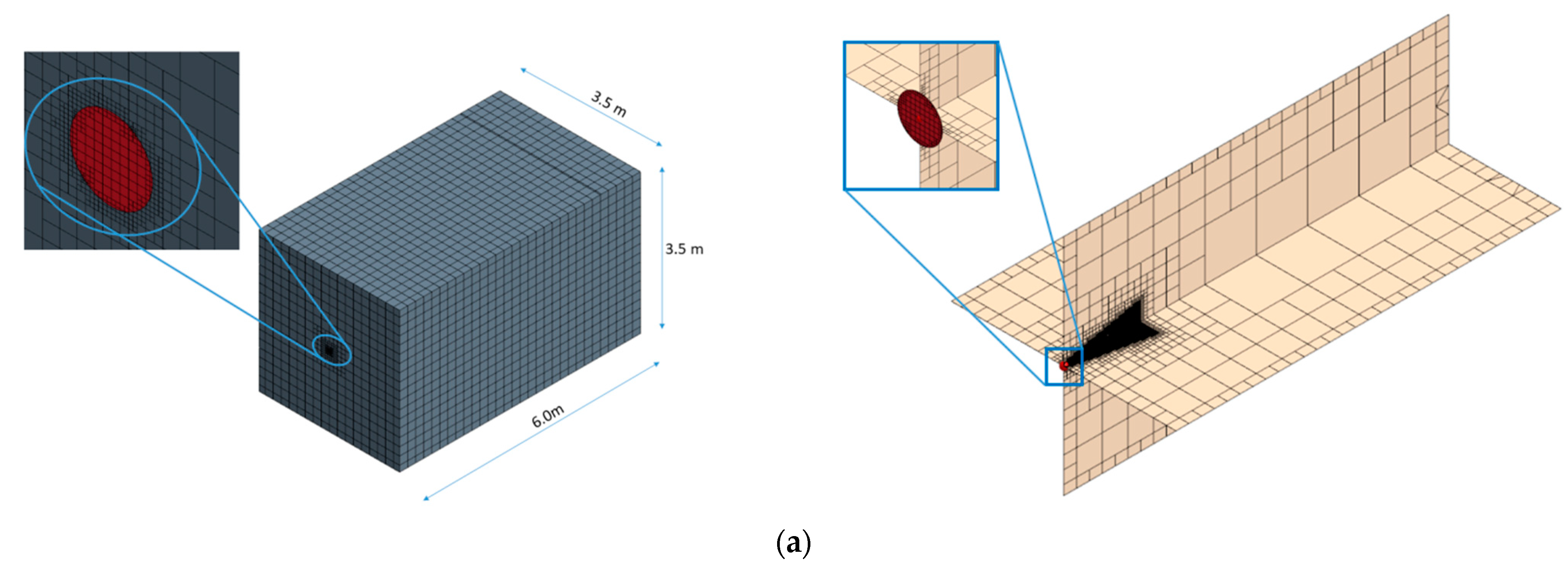
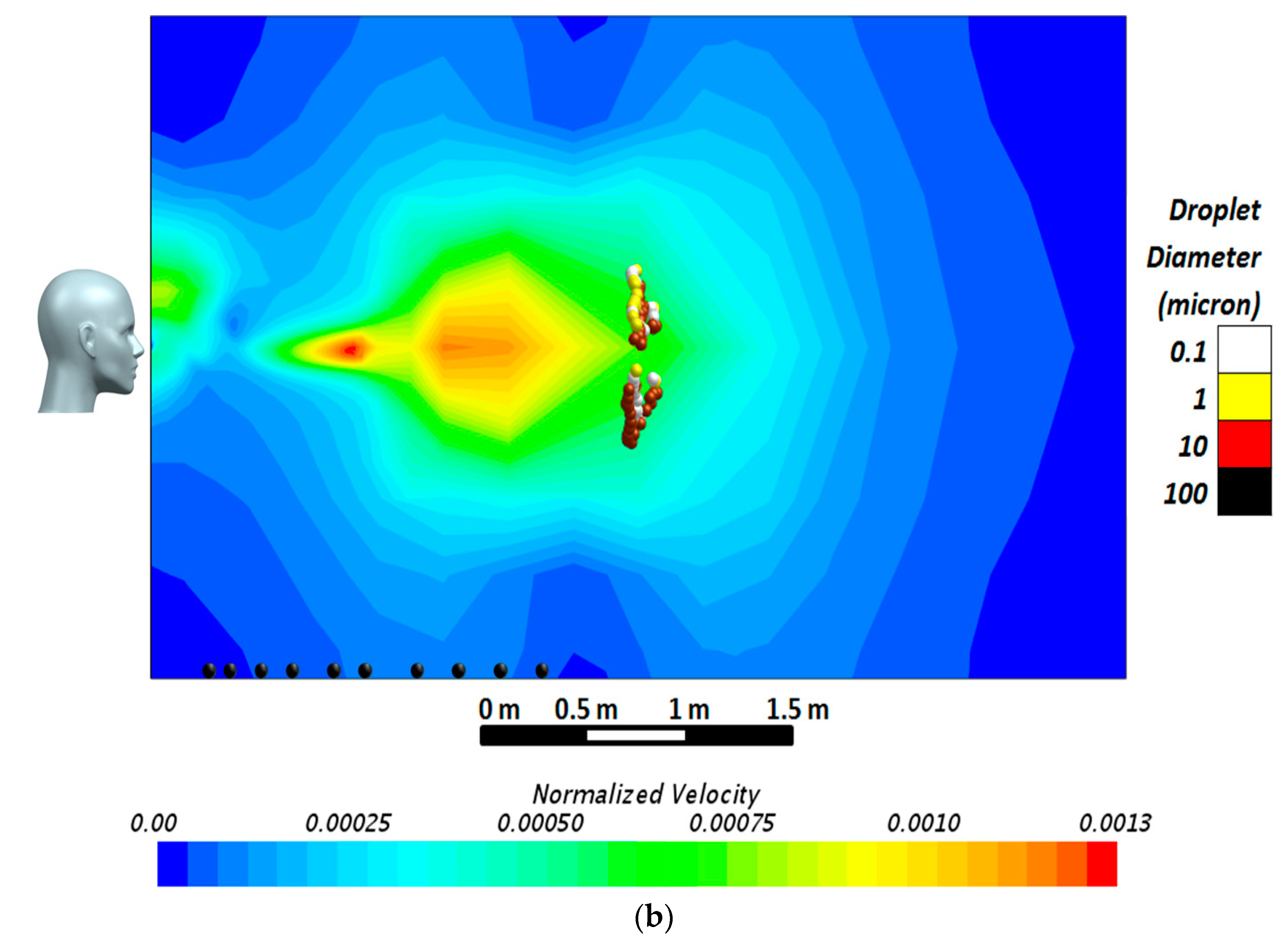
The computational domain was a 3.5 × 3.5 × 6 m room (Figure 2a). The dimensions of the domain were selected after a series of preliminary simulations ensuring the adequacy of the room dimensions for analysis of the airborne behavior of droplets when the exhalation jet’s normalized velocity reaches the value of 0.001. It should be noted that since the measured velocities in all the sneeze or cough experiments depend on the patients’ characteristics (sex, age, weight, body type, etc.), a velocity profile normalized with respect to the sneeze or cough velocity at the location of the mouth can provide a better non-dimensional tool for comparison. In the present research, the exhalation jet velocity at the inlet was used to normalize the velocity field inside the domain. These simulations were performed for different droplet sizes from 0.1 to 100 μm. The results of the simulations, conducted within a wide time span, implied that after a long period of simulations, droplets with a diameter of 10 μm or below had become airborne, traveling up to 6 m from the emitting surface with a terminal velocity below 0.02 m·s⁻¹, while droplets with a diameter of 100 μm regimented at much smaller distances of about 1 m from the jet inlet. The size of the final domain together with the velocity contour of the simulated air jet is presented in Figure 2b.

The respiratory droplets were released from a circular area located at the center of the 3.5 × 3.5 m wall with a diameter of nearly 1.2 cm, which aligned with the reported values in the literature [29,30,31]. The front boundary against the source was an outlet and the rest of the surfaces were considered as solid walls with no-slip boundary conditions (see

Table 1. The boundary conditions of the validation case.

Boundary Type	Boundary Condition	Boundary Value	Air Density	Air Dynamic Viscosity
Inlet	Velocity inlet	20 m·s−1	1.184 kg·m−3	1.855 × 10−5 Pa·s
Outlet	Outlet pressure	1 bar
Walls	No-slip	-	-

). The Lagrangian droplets (discrete phase) were assumed to have spherical shapes and were initially composed of 3% non-evaporative and 97% evaporative mass fractions. The non-volatile fraction had a density of 1280.8 kg·m⁻³ and a specific heat transfer of 2404.6 J·Kg⁻¹·K⁻¹ at the standard state temperature of 298.15 K. On the contrary, the evaporative fraction was assumed to have material properties equal to those of water (density of 997.6 kg·m⁻³, specific heat transfer of 4181.7 J·Kg⁻¹·K⁻¹ at the same standard state temperature). In addition, the saturation pressure of the evaporative fraction was set to 3170.3 Pa. Having assumed the multi-component droplets, the mass-weighted mixture was used for the calculation of the density and specific heat of each droplet. In addition, regarding the boundary condition for each droplet’s outer surface, it was assumed that the droplets would stick to any wall surface of the room as they reached them. The Lagrangian model also included the Schiller–Naumann drag force coefficients and pressure gradient force to accurately simulate the droplets’ trajectories.

The background air was simulated as a non-reactive ideal gas, composed of standard air and some amount of water vapor depending on the relative humidity of each case. The dynamic viscosity, specific heat, and molecular weight of air were assumed to be 1.855 × 10⁻⁵ Pa·s, 1003.6 J·Kg⁻¹·K⁻¹, and 28.97 Kg·Kmol⁻¹, respectively. Like the Lagrangian model, the weighted mixture method for the Eulerian model was employed for the calculation of the air–water mixture. With all the previous settings, the cases were solved on a computer cluster at Sogang University using 24 computational cores with Xeon(R) 2.20 GHz CPUs. The typical simulation time for 60 s was about 15 h.

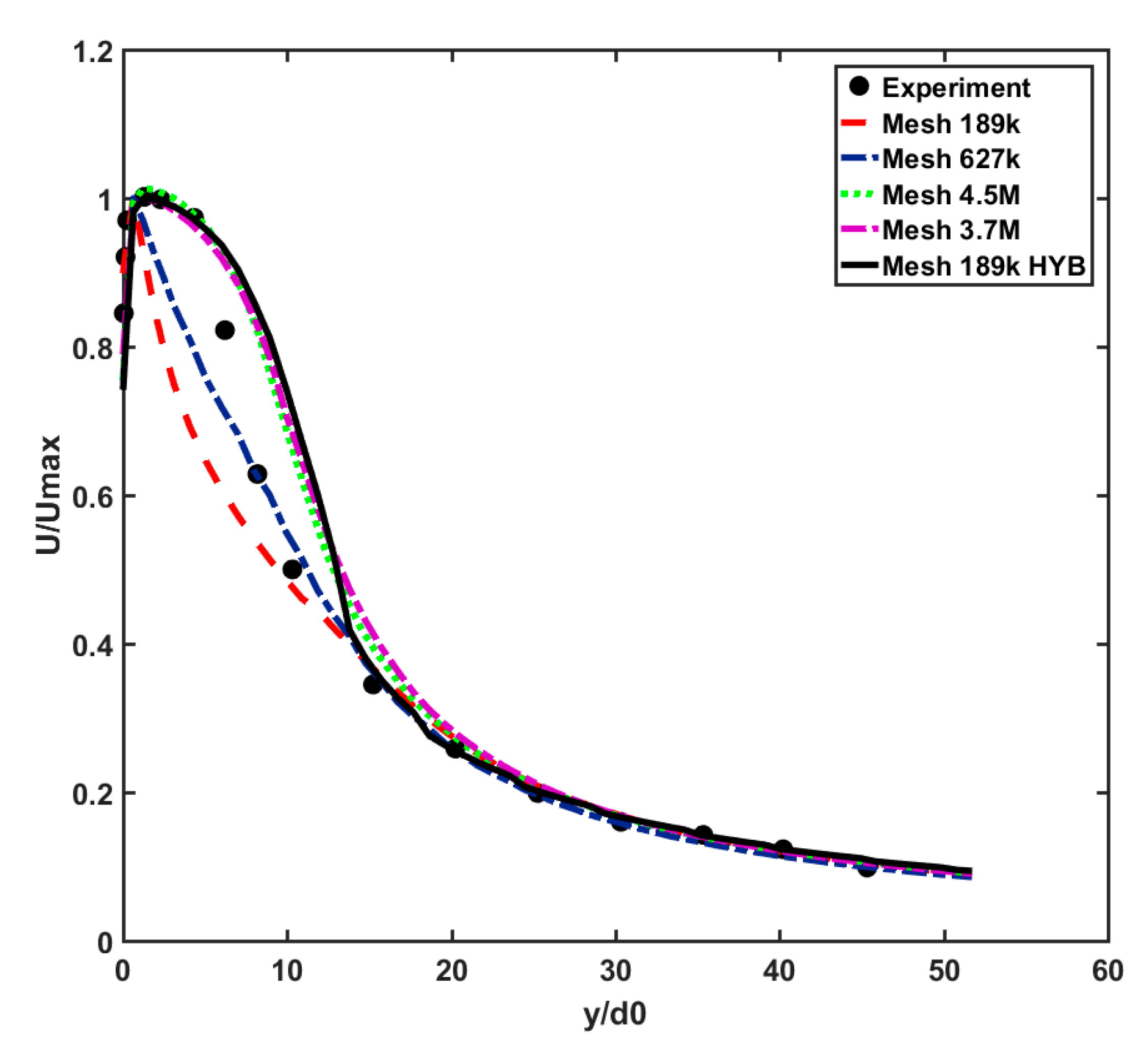
A mesh sensitivity analysis was performed to ensure the mesh independence of the CFD results and for obtaining the optimal computational grid to be used for modeling various cases. For this part, the flow velocity in the far-field zone (i.e., the distance where y/d₀ > 20 from the mouth) was investigated, and the normalized results were validated against the experimental results [36]. The inlet velocity had spanwise (along with discharge hole radii) as well as streamwise (centerline) velocity profiles with the maximum value of 20 m·s⁻¹. It should be noted that the validation case of the Eulerian model was in the isothermal condition. Different mesh resolutions with hexahedral cells were investigated, ranging from 189 k cells to 4.5 M cells, as shown in Figure 2a. The optimal mesh, 189k-HYBcase, has minimum and maximum cell sizes of 0.06 and 0.2 m, respectively, while its surface growth rate is 2.0. This results in a dense mesh of between 0.78 mm (minimum) near the mouth and 0.8 m (maximum) at the central part of the domain. To ensure the accuracy of the results near the walls, the “All Yplus” option was activated, enabling an automatic blending function between low and high Reynolds number wall treatment methods for the calculation of turbulence qualities, such as dissipation, production, and stress tensor [37]. The summary of the applied boundary conditions to validate the Eulerian model is presented in Table 1.

The CFD solver used a double-precision finite volume approach with a second-order discretization scheme. It also contained an energy coupling method (required for evaporation) with implicit integration.

To assess the accuracy of the centerline velocity, four validation metrics, including the factor of two observations (FAC2), hit rate (q), fractional bias (FB), and normalized mean square error (NMSE), were calculated. These metrics are defined as follows:

$$FAC2=\frac{1}{n}{\displaystyle \sum }_{i=1}^n{N}_i$$

(12)

where N_i is calculated as follows:

$$N_i=\{\begin{array}{cc}\hfill 1& \hfill for 0.5\le \frac{P_i}{Q_i}\le 2\\ \hfill 1& \hfill for\left|Q_i\right|\le Wand\left|P_i\right|\le W\\ \hfill 0& \hfill otherwise\end{array}$$

$$q=\frac{1}{n}{\displaystyle \sum }_{i=1}^n{N}_i$$

(13)

with

$$N_i=\{\begin{array}{cc}\hfill 1& \hfill for\left|\frac{P_i-Q_i}{Q_i}\right|\le D\\ \hfill 1& \hfill for\left|Q_i-P_i\right|\le W\\ \hfill 0& \hfill otherwise\end{array}$$

$$FB=\frac{\langle Q\rangle -\langle P\rangle }{0.5\left(\langle Q\rangle +\langle P\rangle \right)}$$

(14)

$$NMSE=\frac{{\langle \left(P-Q\right)}^2\rangle }{\langle Q\rangle \langle P\rangle }$$

(15)

where Q_i and P_i are the measured and computed values of a given variable, respectively; n is the number of available data points, and W and D are the relative uncertainty and repeatability of the calculated data and their values for velocity assessments are 0.05 and 0.25, respectively. The angular brackets of the FB and NMSE equations represent the average of all measured points [33,34].

Table 2. Validation metrics for different mesh sizes.

Mesh Configuration	FAC2	q	FB	NMSE
Ideal Values	1	1	0	0
4.5 M mesh	1	0.875	−0.032	0.012
627 k mesh	1	1	0.074	0.017
189 k mesh	1	0.875	0.092	0.042
189 k-HYB mesh	1	0.875	−0.030	0.027
3.7 M mesh	1	0.875	−0.040	0.020

shows the results of the validation metrics calculated at the centerline velocity diagrams of Figure 3.

According to Table 2, while FAC2 and q give nearly the same values for different mesh sizes, the FB and NMSE values exhibit more sensitivity to the selected computational grids. For instance, applying a hybrid strategy to a mesh size of 189 k considerably improves the FB and NMSE values from 0.092 and 0.042 to −0.03 and 0.027, respectively, which are close to those of the case with 3.7 M cells. This implies that 189k-HYB is an optimal choice for conducting the simulations, providing the best accuracy while minimizing the CPU cost.

3. Risk Assessment Method (RAM)

The risk of airborne disease transmission at each point of a domain is related to the summation of the virus-laden droplets passing through the point within a specific period. Thus, the time-dependent spatial risk of infection can be estimated by the temporal accumulative number of droplets passing through each point in the space. Therefore, in this section, an algorithm is developed to count the accumulated number of droplets at each location downstream of the released respiratory jet.

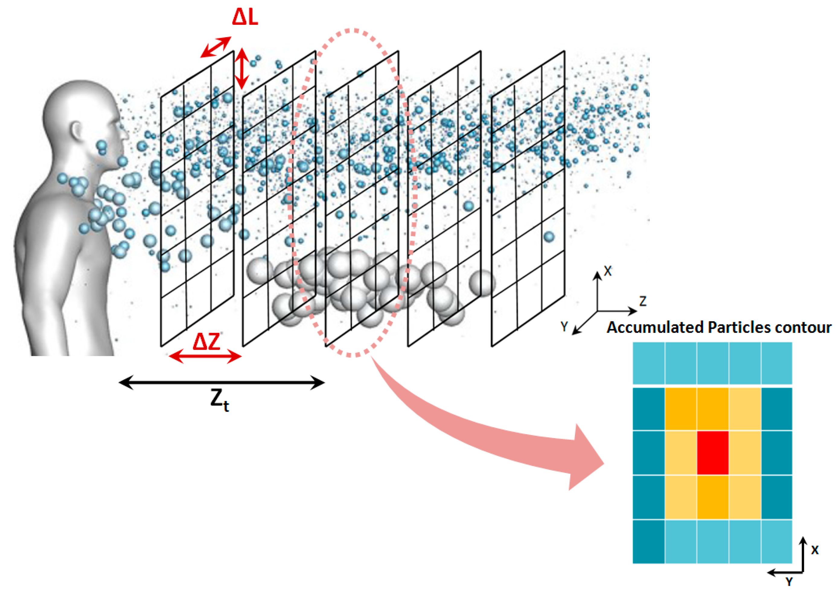
Since exhaled flows contain different droplet sizes, from sub-micron to hundreds of microns, the CFD solver may produce a table of information for each droplet size class at every time step, including position and velocity components as well as the computational grid coordinates. The length of this table depends on the number of defined droplet parcels. The algorithm defines multiple vertical planes at certain distances from the mouth (Z_t), as is shown in Figure 4. The planes are then divided into multiple facial cells. In the next step, the algorithm counts the number of droplets passing through each cell at each time step. 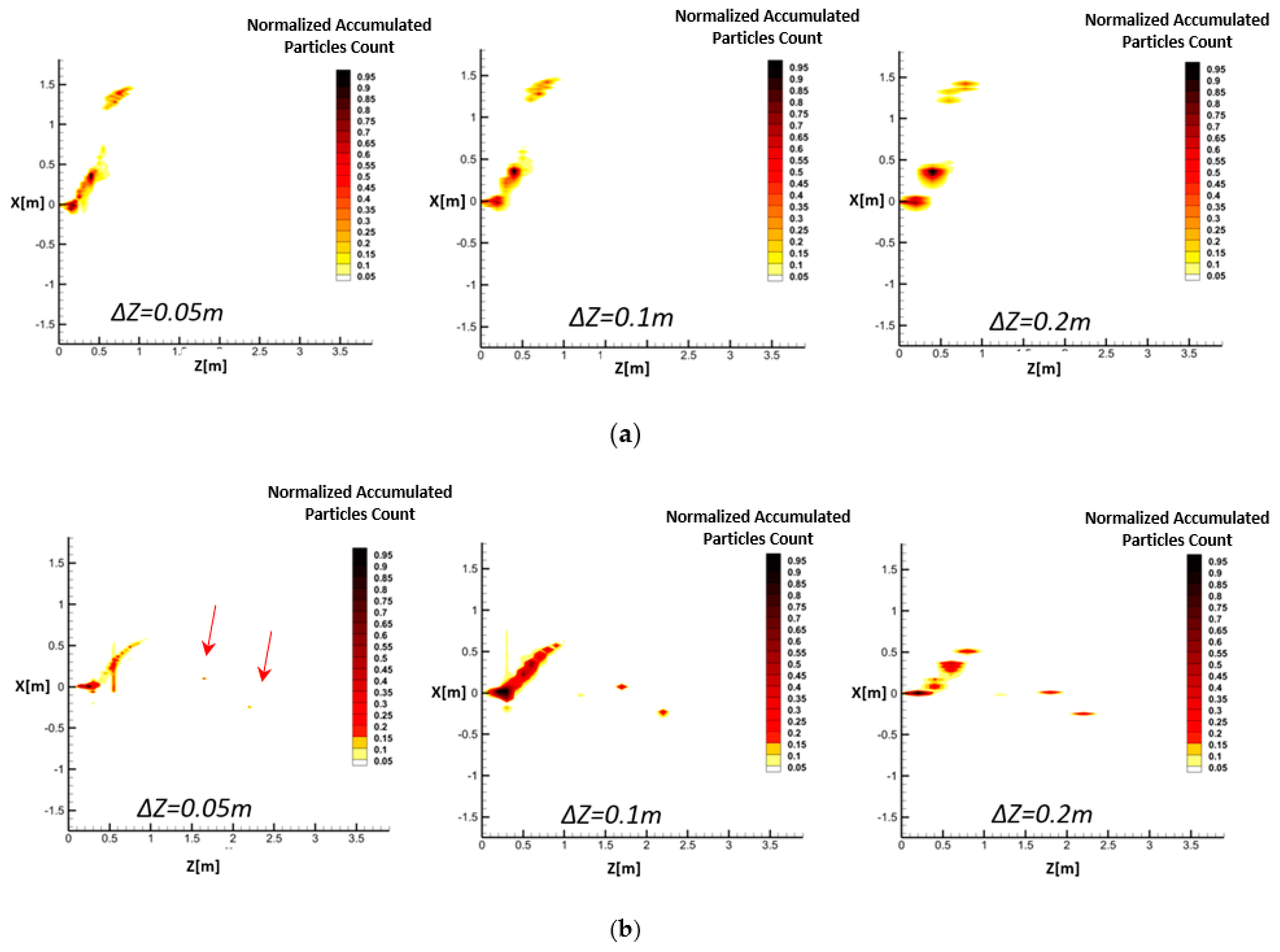According to Figure 4, calculation of the accumulated number of droplets in the field needs a separate 3D meshing with a coarser resolution than that of the CFD model, which is called a “secondary mesh”. Accordingly, the ∆L and ∆Z shown in Figure 4 present the resolution of the secondary mesh.

After constructing the secondary mesh, by using the transient CFD data for the simulation period of 0 to t₁, the proposed algorithm calculates the accumulated number of droplets passing through each of the facial cells within the secondary mesh. As shown in Figure 4, the droplets that pass the plane $Z_t$ at $t_i$ (while not having reached it at $t_{i-1}$) should be identified and counted for each vertical plane of the secondary mesh. Here,$t_i$ and $t_{i-1}$ represent two consecutive times at which the CFD transient data are collected. For this purpose, the droplets’ positions at the previous time step are approximated using the following equation:

$$Z_{t_{i-1}}=Z_{t_i}-V_{z,t_i}\times dt$$

(16)

where $Z_{t_i}$ and $Z_{t_{i-1}}$ are the positions of each droplet at $t_i$ and $t_{i-1}$ in the Z-direction shown in Figure 4, respectively, which are obtained from CFD results; $V_{z,t_i}$ is the z component of each droplet’s velocity vector at $t_i$, and dt is the CFD solution time step. In other words, $Z_{t_i}$ and $Z_{t_{i-1}}$ are the instantaneous positions of droplets according to the CFD solver time step ($dt$). $Z_{t_i}$ is known and $Z_{t_{i-1}}$ is predicted by Equation (16).

Assuming that dt is small enough, $V_{z,t_i}$ can be assumed to be constant from $t_{i-1}$ to $t_i$. By approximation of the Z location of each droplet in the previous time step ($Z_{t_{i-1}}$) and its current location ($Z_{t_i}$), the droplets passing through the plane $Z_t$ between $t_{i-1}$ and $t_i$ can be identified.

$$d{t}^{*}=\frac{\left(Z_{t_i}-Z_t\right)}{V_{Z,t_i}}$$

(17)

In Equation (17),$d{t}^{*}$ is the time required for each droplet to pass the plane that is positioned at $Z_t$, which is different from the CFD solver $dt$. Therefore, $Z_t$ possesses only discrete values depending on the resolution of the secondary mesh. $X_t$ and $Y_t$ are in-plane estimated positions of droplets, while $X_{ti}$ and $Y_{ti}$ are their instantaneous positions inside the domain.

In the next step, the algorithm finds the $X_t$ and $Y_t$ coordinates of the point in the plane $Z_t$ where the droplet crossed the plane $Z_t$. The X and Y positions of each droplet passing through the plane $Z_t$ can be determined as follows:

$$X_t=X_{t_i}-V_{X,t_i}\times d{t}^{*}$$

(18)

$$Y_t=Y_{t_i}-V_{Y,t_i}\times d{t}^{*}$$

(19)

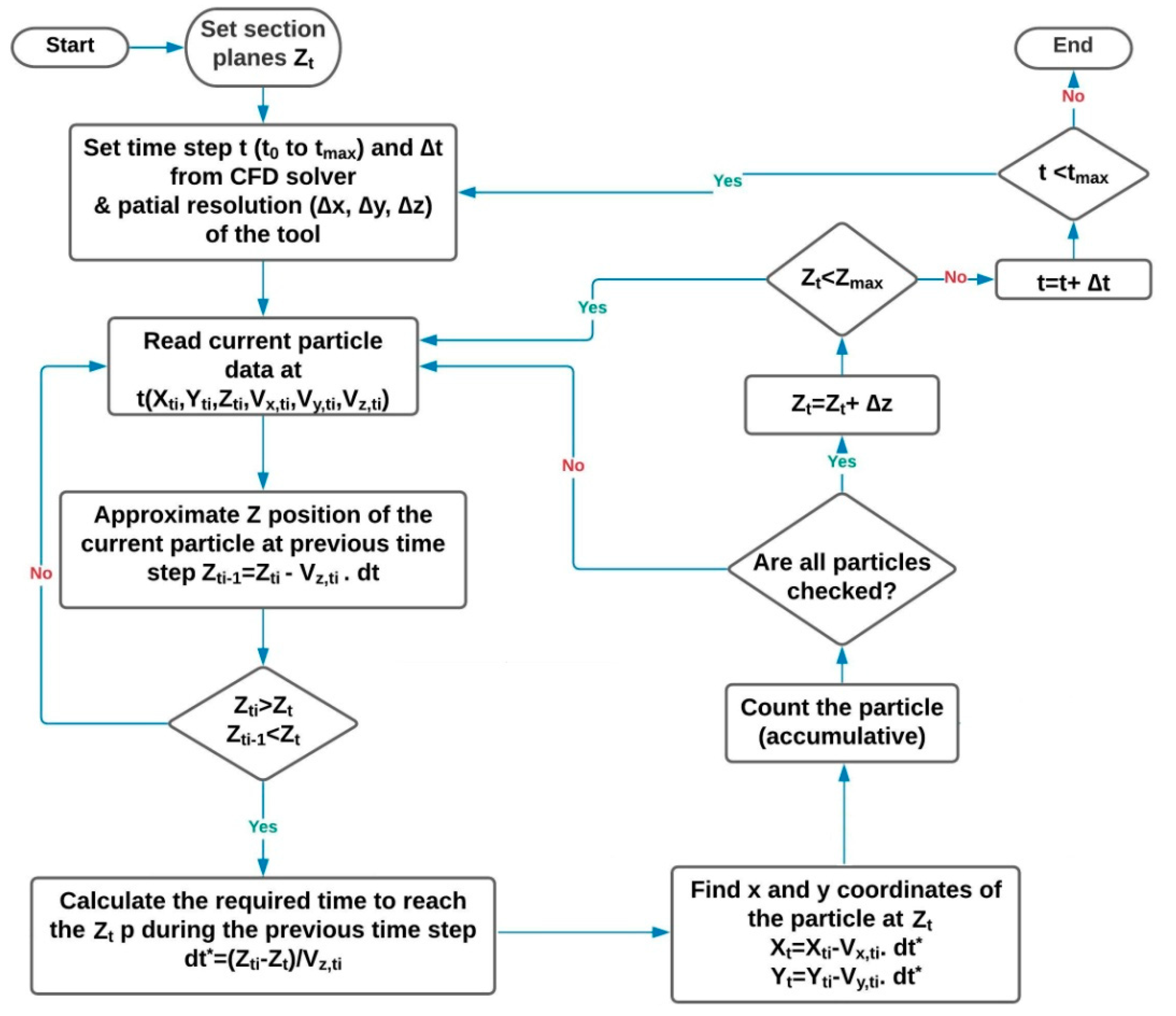
where $X_{t_i} \mathrm{and} Y_{t_i}$, represent the position and $V_{X,t_i}$ and $V_{Y,t_i}$ are the velocity components of the droplets obtained from the transient CFD output data file at $t_i$ in X and Y directions. The graphical representation of the abovementioned procedure for the RAM is presented as a flowchart in Figure 5. A computer program code was written in MATLAB software for post-processing of the CFD simulations based on this flowchart.

In fact, according to Figure 5, $Z_{t_{i-1}}$ is compared with Z_t at each time step to see if it passes the plane Z_t within dt. If yes, Equation (17) is used to estimate the time required for that (i.e., dt*). Then, the calculated dt* is applied to calculate the in-plane positions of droplets (X_t and Y_t) using Equations (18) and (19).

By following this procedure, one can understand how many droplets passed through different facial cells in a certain plane $Z_t$ from $t_{i-1}$ to $t_i.$ By repeating this process for all the time steps between the beginning of a respiratory event CFD simulation and an arbitrary time, the temporal accumulated number of droplets passing through different facial cells can be resolved. This generates droplet number contours similar to those schematically shown in Figure 4. Eventually, following a selected clinical threshold for the minimum number of droplets in an epidemic model (here, it is 100 droplets [27]), it is possible to perform a risk assessment of safe distances. Therefore, only regions with an accumulated number of passing droplets higher than 100 are considered risky areas.

4. Case Studies

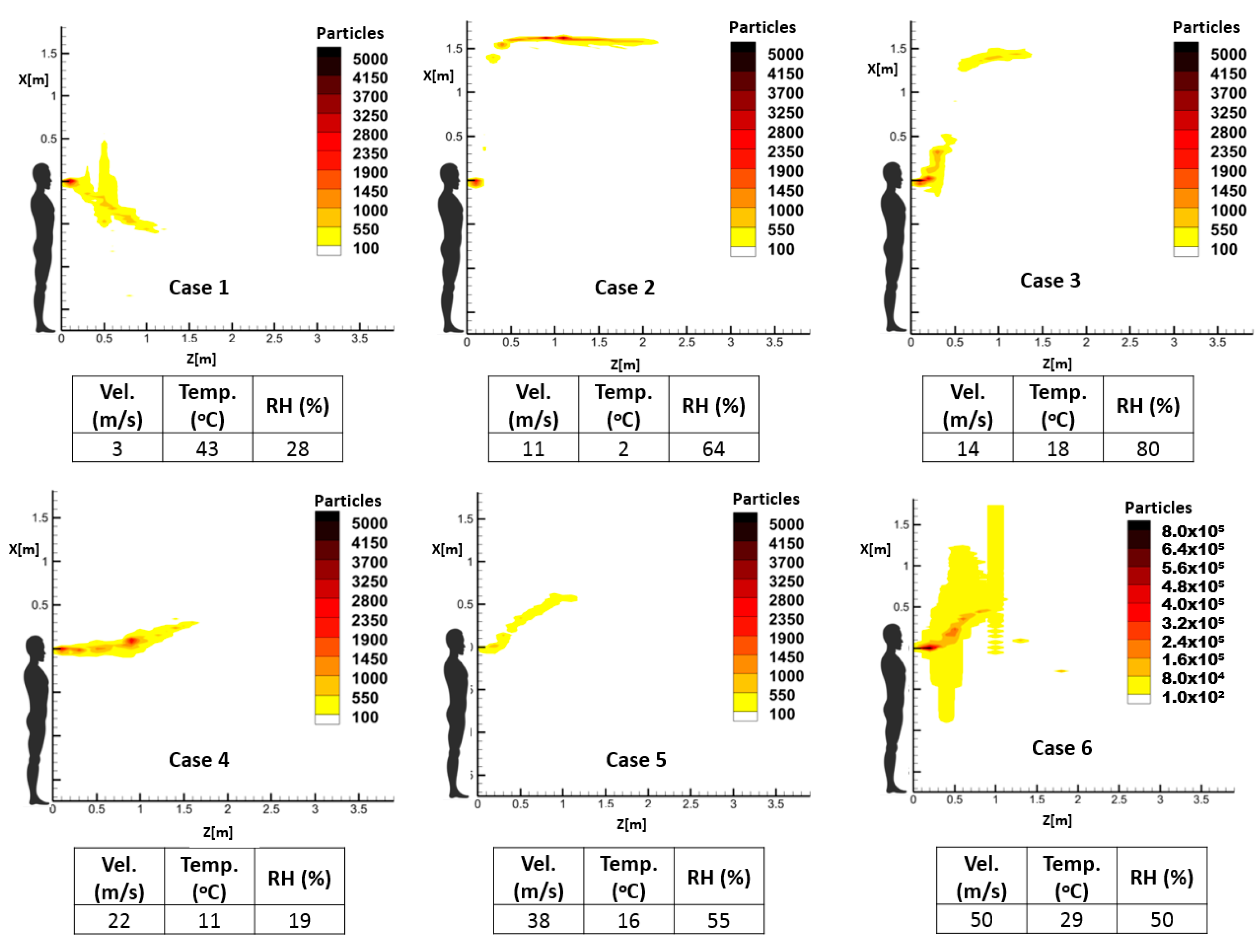
Different exhalation activities are modeled using boundary conditions describing pathogen bio-sources, which are referred to in several related clinical research works [35,38,39]. This information includes the temporal velocity profile, flow rate, and distribution of droplet size in different modes of respiratory events, namely cough, and sneeze. Since respiratory events are modeled as exhaled droplets that immediately evaporate when they are discharged to the environment, the temperature and relative humidity of the space can deeply influence the evaporation and thus the dispersion pattern of the droplets. Therefore, droplets’ velocity, the temperature and relative humidity of the space for some sample case studies are introduced in

Table 3. Characteristics of the defined exhalation scenarios.

Case Number	Exhalation Mode	Exhalation Jet Maximum Velocity (m·s−1)	Temperature (°C)	Relative Humidity (%)
1	Breathing	3	43	28
2	Cough	11	2	64
3		14	18	80
4	Sneeze	22	11	19
5		38	16	55
6		50	29	50

. These parameters were selected to represent different spreading patterns. It should be noted that in these cases, the background velocity of the target environment is not considered. The CFD results of the case studies were then processed using the novel proposed risk assessment algorithm. It should be noted that the exhalation jet temperature of all the following cases was set as 37 °C. According to the reported velocity ranges in the literature [36,40], different scenarios were defined as shown in Table 3 to represent a range of respiratory events to evaluate the performance of the proposed RAM. Moreover, the droplet number and size distribution of the scenarios were adapted from experimental studies [36,37].

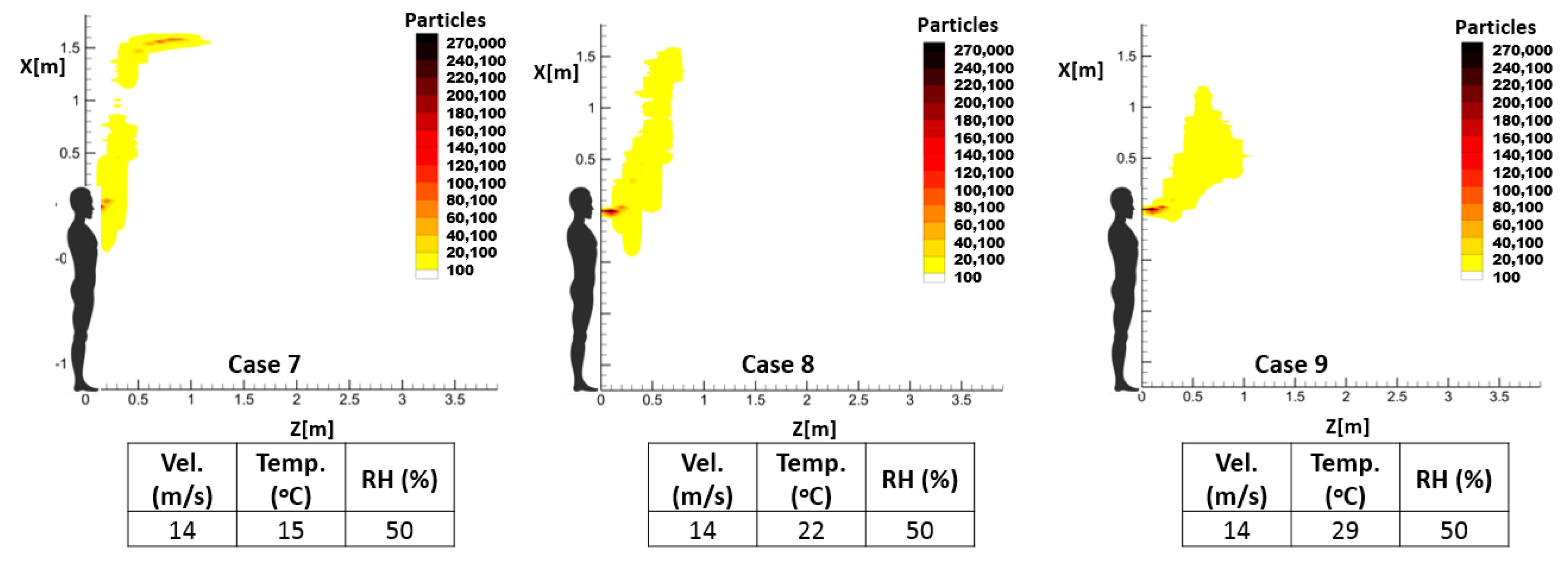
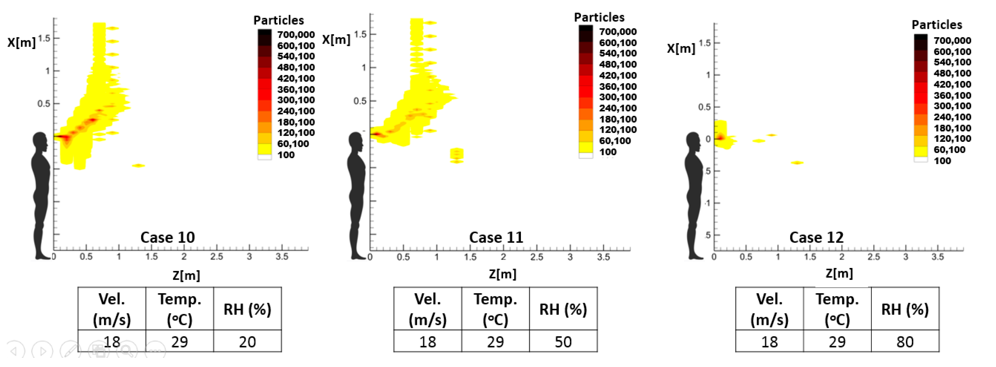
As mentioned earlier, the temperature and relative humidity of the environment has an important influence on the spread pattern and consequently the propagation of infective pathogens. Thus, investigating the impact of these environmental parameters on the accumulative distribution of droplets and, consequently, the high-risk zone will demonstrate one notable application of the proposed prediction method. For this purpose, three sample cough and sneeze cases were defined to demonstrate the respective impacts of the temperature and relative humidity of the environment, while keeping the other parameters unchanged.

Table 4. Characteristics of the cough and sneeze cases for sensitivity investigations.

Case Number	Exhalation Mode	Exhalation Jet Maximum Velocity (m·s−1)	Temperature (°C)	Relative Humidity (%)
7	Cough	14	15	50
8		14	22	50
9		14	29	50
10	Sneeze	18	29	20
11		18	29	50
12		18	29	80

illustrates the characteristics of these exhalation activities.

Table 5. Characteristics of the cough and sneeze cases for sensitivity investigations [41,42].

Size Range	Size Class/Mean	DNC of Speaking	DNC of Coughing	DNC of Sneezing
2–4	3	4.59	86	0
4–8	6	66.21	1187	7706.95
8–16	12	22.23	444	23,491.91
16–24	20	11.33	144	26,203.62
24–32	28	7.87	54	25,689.82
32–40	36	4.32	50	24,933.4
40–50	45	4.47	41	24,176.97
50–75	62.5	4.57	43	58,344.43
75–100	87.5	3.44	30	33,054.23
100–125	112.5	4.52	36	41,703.14
125–150	137.5	4.31	34	32,540.44
150–200	175	4.52	93	41,588.96
200–250	225	3.85	53	44,129.41
250–500	375	3.45	44	179,257.9
500–1000	750	1.11	30	193,444.3
	Sum	150.8	2368	756,265.5

DNC = Droplet Number Concentration.

includes experimental data regarding the number and distribution of exhaled droplets during different exhalation activities.

5. Results

In this section, the performance of the presented RAM is shown in the estimation of the droplets’ accumulation and spread patterns. Initially, a post-processing procedure was conducted over the CFD data to generate small-size output files imported from the Lagrangian CFD model. It is especially helpful in studies that require an excessive CFD run time. These studies can be focused on either finding a trend for the spread of droplets or performing sensitivity analysis.

5.1. Grid Independence of Risk Assessment Model

Reliable prediction of the accumulated number of droplets in the airflow field must be independent of the size of the secondary mesh (i.e., ∆L and ∆Z). To assure this independence, the impact of changing ∆L and ∆Z was studied separately in a cough and a sneeze scenario. For both events, ∆Z was assigned to be 0.1 m, and the results of the risk assessment were calculated for ∆L values of 0.01, 0.02, and 0.05 m. The calculated spread lengths were then compared to assess the mesh independence of ∆L. This comparison is depicted in Figure A1a,b, which shows the normalized accumulated number of droplets at t = 80 s. These figures confirm the mesh independence of ∆L, as the changes seen in different meshes are negligible.

The other important parameter of the secondary mesh is the distance between Z-constant planes (∆Z). To investigate this parameter, for a constant value of ∆L = 0.02 m, the results of three different ∆Z values of 0.1, 0.2, and 0.5 m were examined for two respiratory events of cough and sneeze. As seen in Figure A2, the changes in predictions between ∆Z values of 0.1 and 0.2 m are quite small, whereas there is a considerable discrepancy when ∆Z is 0.5 m. Hence, ∆Z was set as 0.1 m for producing the rest of the results in this paper.

5.2. Spreading Pattern of Respiratory Jets

The proposed RAM can be used to estimate the horizontal and vertical spreading distances of the temporal accumulated risk factor for respiratory jets of various events in different thermal conditions. Figure 6 illustrates a 2D representation of risky regions with an accumulated number of droplets higher than 100 for the case studies defined in Table 3 after 80 s. Output data of the CFD simulations were imported to the risk calculation code to find accumulated droplet distributions as well as high-risk zones. For all the introduced cases, it was assumed that both the infected person and susceptible subjects will remain in the same environment during the intended exposure time. As seen in Figure 6, different respiratory events can produce different spreading patterns in risky regions. The obtained behavior of risky regions shows how the safety distance from an infected person strongly depends on the respiratory event as well as the environmental conditions. For instance, while the horizontal spread of pathogens in Cases 2 and 3, representing cough events according to Table 3, will not be considered a threat to susceptible individuals, the spreading behavior observed in Case 4, a sneeze event, is nearly horizontal and can pose a serious risk to others within the 1.8-meter distance from the infected person. In other words, a safe inter-person distance in Cases 2 and 3 can be as low as 0.5 m because of the high tendency of these exhalation jets to rise upward. However, a quite different trend is seen in Case 4. The vertical spread of the mentioned cases is also an important parameter to consider when evaluating the risk factor. Higher values of vertical spread in these cases can impose a health risk on ventilation systems, possibly through the ducts, and therefore have a higher infection probability. The opposite behavior is observed in Case 1 with a downward vertical spread, which indicates a weak airborne dispersion of droplets. Case 6 represents a sneeze event with a very high concentration of droplets ranging from sub-micron to some hundreds of microns, which results in a thick cloud forming highly contaminated space in front of the infected person. This behavior is quite different from the low-width propagations of the other cases observed in Figure 6.

5.3. Safe Distance Calculations

The numerical results of the CFD simulations can be post-processed to provide 3D and 2D projections of the accumulated spread patterns for different exhalation activities. Figure 7 illustrates the 2D and 3D representations of cough spread droplets. Although it is possible to exploit 3D iso-surfaces of droplet counts (Figure 7a), 2D projections(Figure 7b), are more informative and useful to build up a predictive model or perform different sensitivity analyses. Three-dimensional representations of respiratory events also illustrate the lateral propagation of droplets. This is especially important when the lateral safe distance of a susceptible person from an infected person is intended. These 3D data can be applied to build more sophisticated prediction tools, calculating a safe region instead of a simple safe social distance as is the case in 2D investigations. For instance, these 3D safe regions can be applied to spaces in which a relatively high concentration of people is inevitable.

High-risk regions where the number of accumulated droplets is higher than a certain limit can be easily identified with the present RAM. In this regard, when accumulated droplet numbers are calculated throughout the target domain, only regions with a high enough concentration of droplets will be considered as high-risk areas. This necessitates setting a minimum infection dosage. A few medical research works have mentioned the infection minimum dosage. Among them, the value of a minimum of 100 droplets was reported by Karimzadeh et al. [27]. An illustrative example of applying this criterion is presented in Figure 8. The contour image of Figure 8a shows the accumulated distribution of droplets for a 60-s time span inside the target domain. This figure only shows the position of all droplets exhaled during that 60 s. Distinct zones of airborne and falling droplets can be evidently distinguished in this contour. However, risky zones cannot be identified. To find high-risk areas, one should find the regions with enough accumulated droplets within the exposure time of 60 s. Hence, to turn this image into one that presents high-risk areas, regions having accumulated droplet numbers less than the minimum infection dosage should be filtered. Figure 8b, as a result, highlights the regions having the minimum dosage (at least 100 droplets) within the simulation time. It can be observed that the high-risk zone is not necessarily identical to the spatial position of the droplets in the field. For instance, falling droplets seen in Figure 8a, due to their low concentrations in this sample case, are not recognized in the risk zone picture. It should be noted again that what refines Figure 8a to acquire Figure 8b is based on the minimum dosage threshold, which can be changed with respect to the assumed number.

5.4. Instantaneous and Accumulative Concentrations

Unsteady CFD simulation results provide useful information about the position and velocity of each droplet at different time steps. However, they cannot directly confer an insight of risk assessment for the understanding of safe social distances. This is because the risk and infection analyses require the measurement of the overall dosage received by a new host, which needs calculation of the accumulated number of droplets during a definite time span. In other words, instantaneous images of flow field droplet concentrations do not contain any vision of risky zones or safe social distances.

Figure 9 and Figure 10 were generated through post-processing of CFD simulations to provide a comparison between instantaneous and accumulative distributions of the number of droplets inside the computational domain for a cough and a sneeze event, respectively. According to Figure 9, at t = 20 s, a region with falling droplets within half a meter from the source can be observed in instantaneous mode, while this is not the case in its accumulated contour. The reason is that the accumulative calculations detect the droplets passing through vertical Z-constant planes. These droplets, however, can barely pass through these planes, so they are not captured. Since they have no contribution to the risk factor, this will not influence the accuracy of the outlined RAM predictions. A similar trend can be seen in Figure 10, which exhibits a sneeze case.

According to Figure 10 (bottom), falling droplets observed at time-resolved contours are not seen in accumulated contours at the top. The reason is that free-falling droplets, even with high concentrations, cannot be captured using the RAM. This, however, does not cause any considerable error in safe social distance calculations since they have no contribution in the spread patterns of airborne pathogens.

As seen in Figure 9 and Figure 10, falling droplets are not detected by the RAM. However, this is not an indication of any error in the calculation of safe social distance. The reason is that if falling continues, the falling droplets leave the domain with no horizontal propagation and, consequently, no contribution to the airborne spread of pathogens. On the other hand, if falling droplets become airborne because of evaporation, their impact on the horizontal spreading of pathogens will be captured by RAM as soon as they gain a horizontal velocity component.

5.5. Time History of Spreading Patterns

Most exhalation activities such as coughing, sneezing, and even breathing are normally associated with temporal discharge fluxes of viral loads. This implies that in these cases, a safe distance is closely tied with the exposure time. Hence, the determination of a safe distance in such cases strongly depends on the exposure time for the new host; the shorter the exposure time, the smaller the social distance will be. On the other hand, most predictive tools rely on steady flow and fully mixing conditions, which is not the case for short-duration activities such as sneezing and coughing. These issues are addressed by the present RAM, which brings more flexibility to the conventional definition of social distancing measures. Figure 11 shows the variation of high-risk regions with time for Case 4, where the role of exposure time in expanding the risky region can be seen. The figure shows that the safe distance varies from almost 0.5 to nearly 1.8 m as the exposure time rises from 10 to 80 s. Hence, depending on the contact time between an infected person and a susceptible one, the safe distance will be flexible to some extent.

5.6. Spreading Pattern Cross-Sections

Although the results presented so far are 2D representations of accumulated droplets spreading in the X-Z plane, further 3D representation of the results expressing a more sophisticated description of safe social distance is needed. Figure 12 shows the distribution of accumulated droplets in Z-constant planes (X-Y planes) at different distances from the mouth, varying from Z = 0.1 to 1 m. In this figure, the accumulated distribution of the falling heavy droplets, as well as the small airborne ones, can be distinguished at each plane. Figure 12 also provides useful information on the lateral spread shape and size of droplets at different distances from the infected person. It shows that if an infected person coughs or sneezes, due to the droplet dispersion and scattering, a lateral area of up to 1 m will be highly contaminated and should be considered as a risky zone as well. This is especially crucial when the population of occupants in the target space is relatively large, and different arrangements of people need to be assessed to find the lowest infection risks. The occupied area of Z-constant planes can be used to further develop the concept of social risky distance in a risky region.

5.7. Sensitivity of Spreading to Environmental Conditions

The sensitivity of the spreading pattern to ambient temperature was investigated through cough cases as per Table 4. Figure 13 represents the variation of high-risk zones caused by cough cases 7 to 9 after 60 s.

According to this figure, ambient temperature has an important impact on the propagation of risky regions. As the temperature difference between the exhaled droplets and the environment rises, the upward propagation of droplets declines, and their tendency to horizontally spread increases. Therefore, in this case, the social safe distance varies from 0.5 to nearly 1.2 m after 60 s, when the ambient temperature changes from 15 to 29 °C. A similar investigation was performed on the impact of the relative humidity on high-risk zone patterns caused by a sneeze. For this, the CFD results of sneeze cases 10 to 12 as per Table 4 were used to compute the accumulative distribution of exhaled droplets. The results of the high-risk calculations are presented in Figure 14. These contours show how the relative humidity of the environment can alter the propagation mechanism of droplets. As the relative humidity increases from 20 to 80%, the airborne propagation of droplets and, as a result, the airborne transmission of pathogens weaken, while falling drop regions are intensified as a result of the droplet sizes used according to Table 5. Therefore, the social safe distance risk of infection decreases. These investigations also imply that the proposed RAM is sensitive to parameters defining exhalation activities and can be applied to different parametric studies as well as for developing infection prediction tools.

It is worth mentioning that when the ambient relative humidity is high, the evaporation becomes slower, and hence, more droplets fall because of the gravitational force, thus reducing the risky distance.

6. Concluding Remarks

A new assessment method has been presented to find the time-dependent accumulative concentration of infectious exhaled droplets based on CFD simulations. The CFD calculation results encompass the instantaneous position of droplets, while the infection is associated with receiving a sufficient infective dosage during the exposure time, which necessitates the calculation of the accumulated particles within an arbitrary time interval. For this purpose, transient CFD output data files including the position and velocity vectors of each released droplet are generated. By implementing a secondary mesh for post-processing of the transient CFD data, temporospatial droplet trajectories can be traced via a computational code. The CFD results of different respiratory events in terms of exhaled jet maximum velocity as well as environmental conditions were applied to the proposed framework to calculate droplets’ spreading lengths. The following remarks can be concluded:

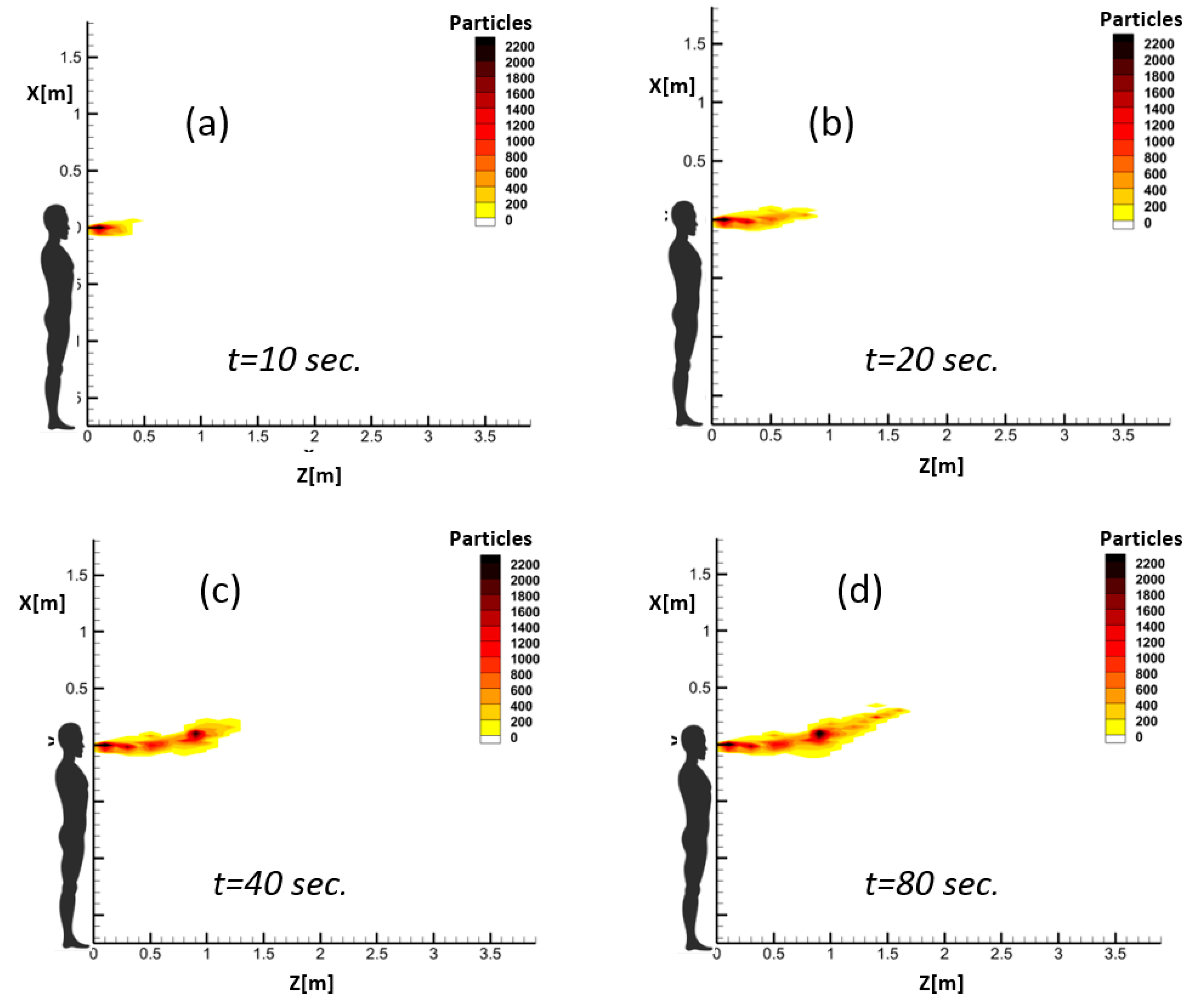
• The obtained results indicate that the proposed RAM method can successfully capture different respiratory events. Hence, the length and height of spread as well as the overall behavior of different exhalation jets can be studied using the proposed RAM.
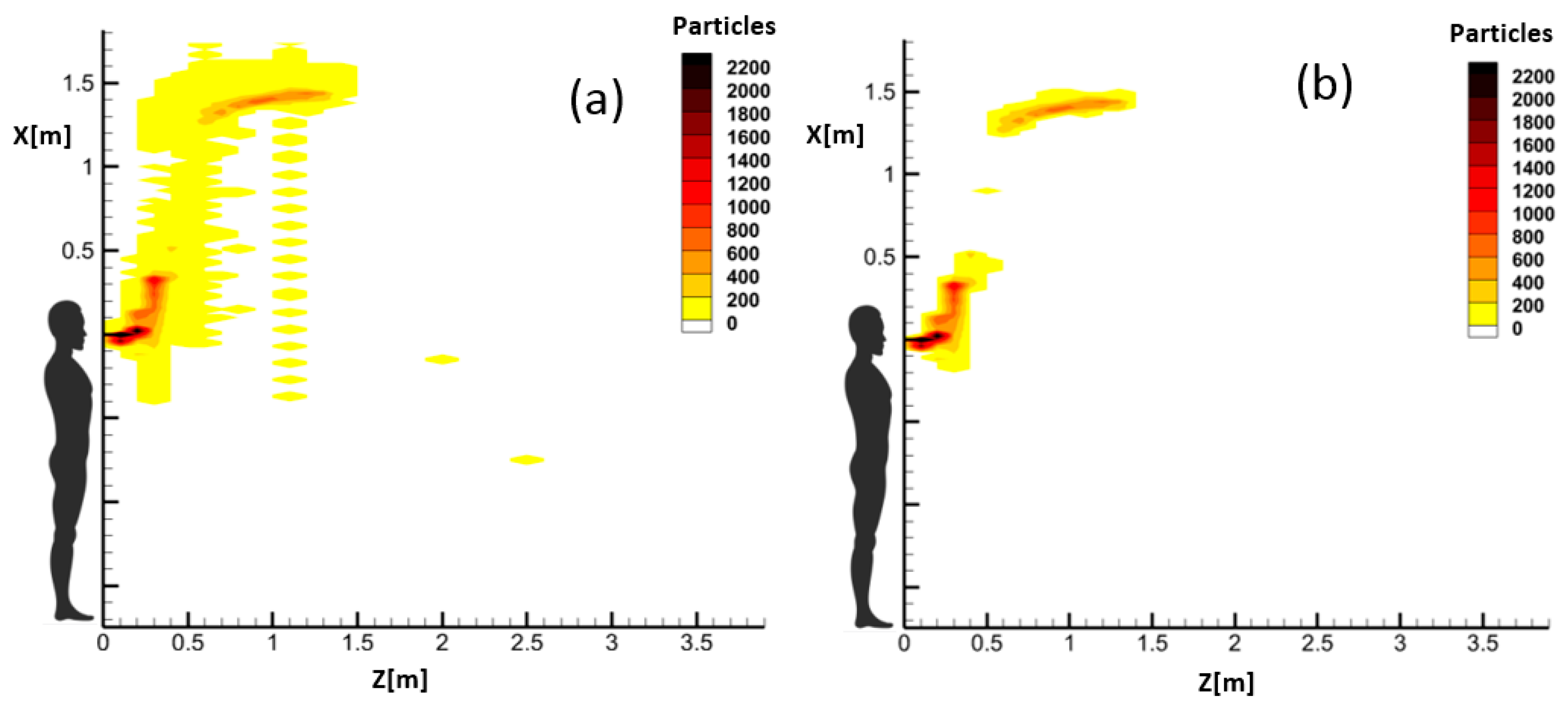
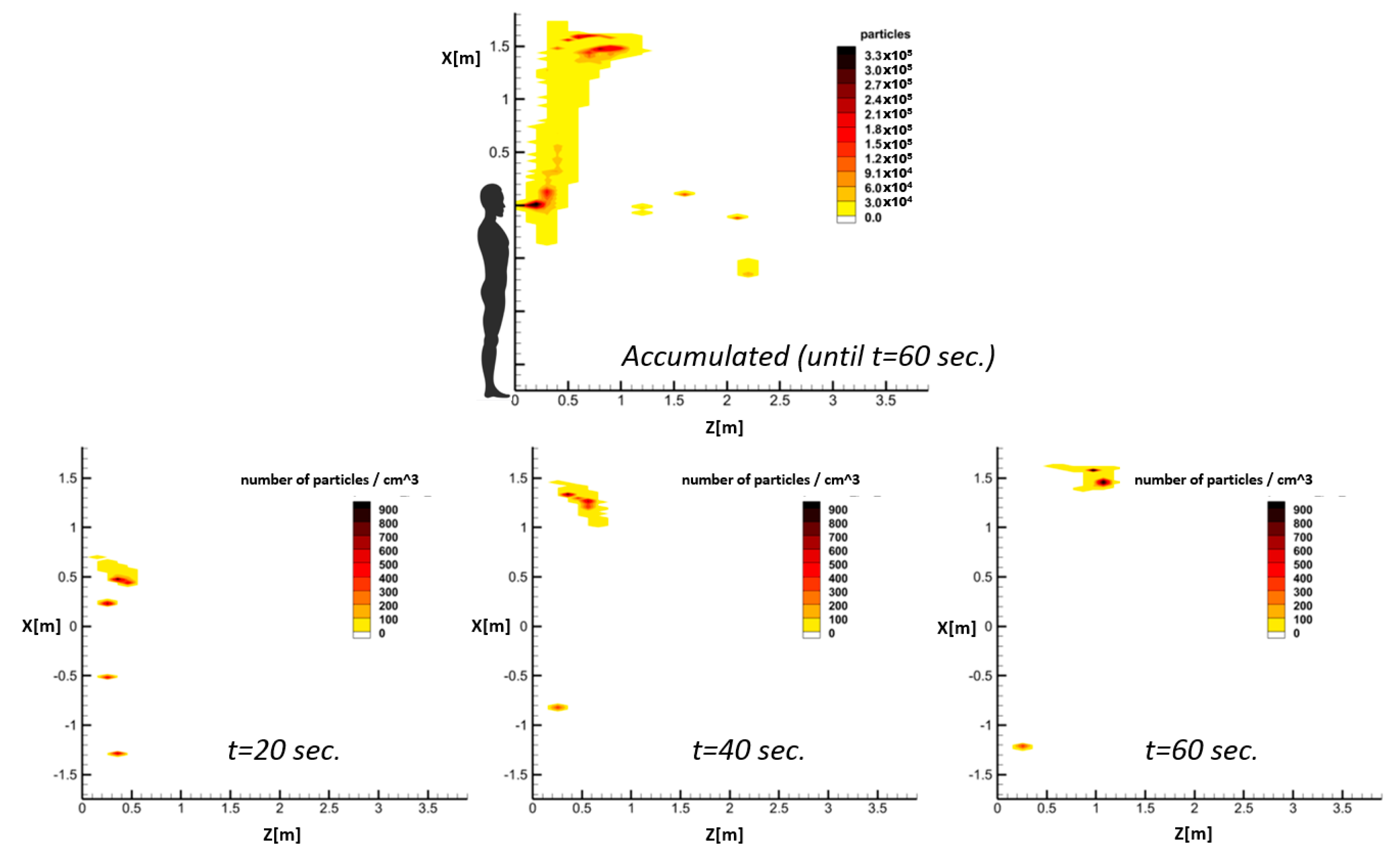
• While the instantaneous CFD output data of droplets can barely provide any information regarding risky and safe zones inside a domain, the proposed model can represent the evolution of risky zones in time. Comparison of the instantaneous and accumulated droplets indicated that most of the heavy falling particles do not pass through the Z-constant planes through the field, which is used in the accumulated representation. Since these particles do not contribute to the dispersion of droplets in the domain, this adds no error to the calculated spreading length and height of airborne droplets.
• The proposed RAM can be used to derive safe social distances in terms of exposure time. This is especially important in short-duration respiratory activities such as coughing or sneezing in which considerable viral loads are released by an infected person and the safe distance for susceptible persons depends on their exposure time.
• The calculated results confirm that the sensitivity of the predicted spreading patterns to environmental temperature and relative humidity can be investigated by the proposed RAM. According to selected sample cases, both parameters can influence the propagation length and even the mechanism by which droplets are transmitted inside the environment.

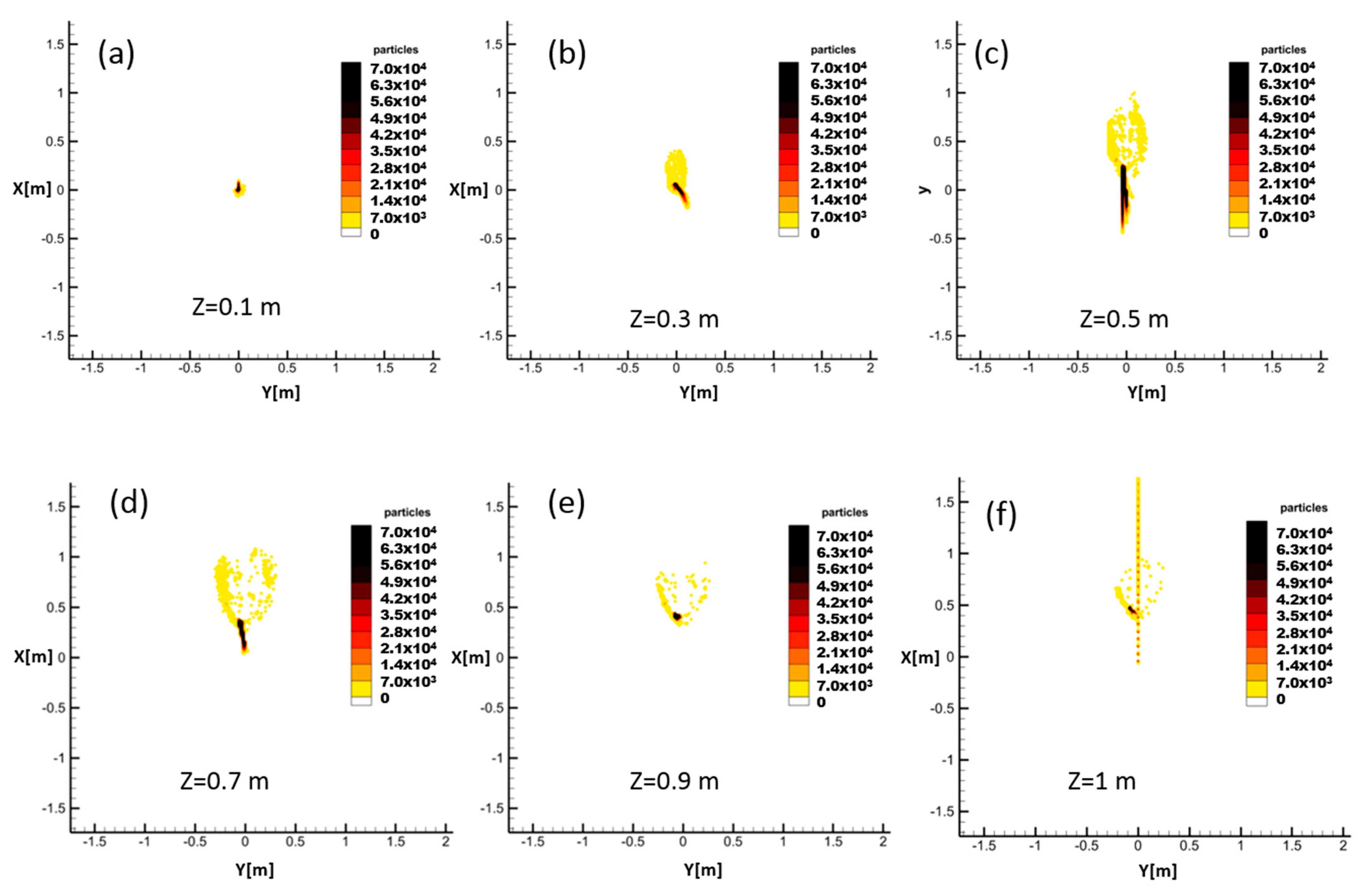
Finally, since this method is a 3D prediction model, it is possible to investigate the cross-section of the spreading pattern of droplets through Z-constant planes. These data can be used to define 3D risky regions. This will be the subject of our future work to add a lateral dimension to risk evaluation and further improve the resolution of social distance calculations. This will be particularly useful for spaces where a high density of people is inevitable. Additionally, this code can be adapted to specify risky volumes, as opposed to safe horizontal distances, including complex flow patterns caused by advection, buoyancy, and gravitational settling of particles.

Among the restrictions of this research work, one can identify the insufficient clinical data on exhalation activities as well as the infective dosage of COVID-19, which has a crucial impact on safe social distance calculations. Another limitation of this work is that the instantaneous position of droplets was approximated based on the available data of the previous time step of the CFD calculations. If the time-dependent position of droplets on each streamline is known, it would result in more precise predictions.

Future work can include an adaptation of this code to risky volumes, as opposed to safe horizontal distance. With complex flow patterns caused by advection, buoyancy and gravitational settling of particles, the risky environment can become complex. Perhaps the entire 3D space around the infection source can be broken down to 20–50 volumes and the risk in each volume can be calculated. In monitoring volumes, you would simply consider the time integral of the number of droplets in each volume at any given time.