Article

Quantification of Regional Ozone Pollution Characteristics and Its Temporal Evolution: Insights from Identification of the Impacts of Meteorological Conditions and Emissions

1
South China Institute of Environmental Sciences, Ministry of Ecology and Environment, Guangzhou 510655, China
2
School of Environment and Energy, South China University of Technology, Guangzhou 510006, China
3
Institute for Environmental and Climate Research, Jinan University, Guangzhou 511443, China
4
Customer Service Center, China Southern Power Grid, Guangzhou 510620, China
*
Author to whom correspondence should be addressed.
Atmosphere 2021, 12(2), 279; https://doi.org/10.3390/atmos12020279
Submission received: 24 January 2021 / Revised: 10 February 2021 / Accepted: 15 February 2021 / Published: 20 February 2021
(This article belongs to the Special Issue Air Quality Management)

Abstract

:
Ozone (O3) pollution has become the major new challenge after the suppression of PM2.5 to levels below the standard for the Pearl River Delta (PRD). O3 can be transported between nearby stations due to its longevity, leading stations with a similar concentration in a state of aggregation, which is an alleged regional issue. Investigations in such regional characteristics were rarely involved ever. In this study, the aggregation (reflected by the global Moran’s I index, GM), its temporal evolution, and the impacts from meteorological conditions and both local (i.e., produced within the PRD) and non-local (i.e., transported from outside the PRD) contributions were explored by spatial analysis and statistical modeling based on observation data. The results from 2007 to 2018 showed that the GM was positive overall, implying that the monitoring stations were surrounded by stations with similar ozone levels, especially during ozone seasons. State of aggregation was reinforced from 2007 to 2012, and remained stable thereafter. Further investigations revealed that GM values were independent of meteorological conditions, while closely related to local and non-local contributions, and its temporal variations were driven only by local contributions. Then, the correlation (R2) between O3 and meteorology was identified. Result demonstrated that the westerly belonged to temperature (T) and surface solar radiation (SSR) sensitive regions and the correlation between ozone and the two became intense with time. Relative humidity (RH) showed a negative correlation with ozone in most areas and periods, whereas correlations with u and v were positive for northerly winds and negative for southerly winds. Two important key points of such investigation are that, firstly, we defined the features of ozone pollution by characterizing the temporal variations in spatial discrepancies among all stations, secondly, we highlighted the significance of subregional cooperation within the PRD and regional cooperation with external environmental organizations.

1. Introduction

The Pearl River Delta (PRD), the largest city cluster in South China, has long suffered from severe air pollution due to rapid urbanization and intensive anthropogenic activities. Following the introduction of a series of stringent air pollution control measures, levels of most atmospheric pollutants in the PRD, such as SO2, NOx, CO, PM10, and PM2.5, have gradually decreased in recent years; however, tropospheric ozone (O3) is the exception and it became the primary pollutant since 2015 and the amount of days exceeding the standard (160 μg/m3) is far more than the other two regions [1,2,3]. After suppressing PM2.5 to levels below the standard concentration, the PRD will now focus on ozone control. As O3 is relatively persistent, it can be transported between adjacent areas, and therefore O3 concentrations at different stations within small areas approach similar levels. Such aggregated distributions can provide insight into the interactions within a small area. However, such investigations, especially quantification of the aggregated distribution, have not been discussed in detail in previous studies.
O3 is formed by the photochemical reaction of the precursors NOx and volatile organic compounds (VOCs) under the action of sunlight [4,5]. The relationships between O3 formation and its precursors are highly nonlinear and have been investigated in detail based on observations or simulations [6,7,8,9,10]. Generally, O3 formation is sensitive to VOCs in urban areas and to NOx in suburban or rural areas [10,11,12]. O3 formation has become less VOC-limited due to the substantial reductions in NOx in urban areas, and there have been several related investigations in the PRD [10,13,14,15,16].
O3 concentrations are related to meteorological conditions [17,18], local production [6,19,20,21], and long-range non-local transport from outside the local area [22,23,24,25]. Several different methods based on simulation models or observations have been used to investigate the influence of these factors [9,24,26,27]. Photochemical reaction rate, precursor emission rate, and transportation of O3 and its precursors are affected by meteorological conditions directly or indirectly. Due to differences in meteorological conditions and precursor emission levels at the various stations, the correlations between O3 concentrations and meteorology vary considerably. Previously, we investigated the long-term effects on O3 levels in the PRD of local and non-local O3 production, differences in meteorological conditions, and differences in precursor emission levels [28]. We concluded that meteorological conditions suppressed O3 increases over the long-term, and local emissions showed different impacts in the northeastern and southwestern of PRD, while non-local sources had similar impacts on the whole area. However, there has been insufficient investigation into the relationships between O3 and meteorological conditions in the perspective of space, especially the long-term spatiotemporal evolution.
Meteorological variables, such as solar radiation, can control the photochemical reaction and affect net O3 production directly, while high temperatures are conducive to O3 production by increasing emission of natural sources biogenic volatile organic compounds (BVOCs), hydroxyl radical (OH) concentrations in the atmosphere, and decomposition of peroxyacetyl nitrate (PAN) [29,30,31]. High O3 concentrations are commonly accompanied by high temperatures, high levels of solar radiation, low relative humidity, and weak winds [32,33,34]. Areas with similar variations in O3 and meteorological conditions are likely to have similar sensitivity to meteorological conditions. This provides a straightforward approach to infer the relationships between O3 and meteorological conditions.
Generally, stations with impacts from local sources are likely to have discrete geographic distributions because of the heterogeneous local emission levels at the different stations, compared with the case of non-local impacts that result from O3 transport by large-scale prevailing winds are removed. Such non-local contribution result in more uniform O3 concentrations at the different stations. Thus, the aggregated distribution of stations affected by local impacts will be strengthened when non-local sources are added. It is unclear whether the aggregation is affected by meteorological conditions, although areas with high precursor levels are more sensitive to meteorological variations [35]. O3 concentrations can be reinforced or weakened by meteorological conditions depending on the mechanisms of O3 formation and transport into or out of the area of the station. Over the long term, the temporal evolution of such aggregation of O3, the roles of meteorological conditions, local and non-local contribution on the aggregated distribution of stations were hardly noted.
In this study, we used spatial analysis based on observation data of the PRD to quantify the extent of aggregation of O3. The temporal evolution of O3 from 2007 to 2018 and the driving factors were then identified. Finally, the spatiotemporal evolution of correlations between O3 and meteorological conditions was examined. These investigations characterize O3 pollution and facilitate its control.

2. Data and Methods

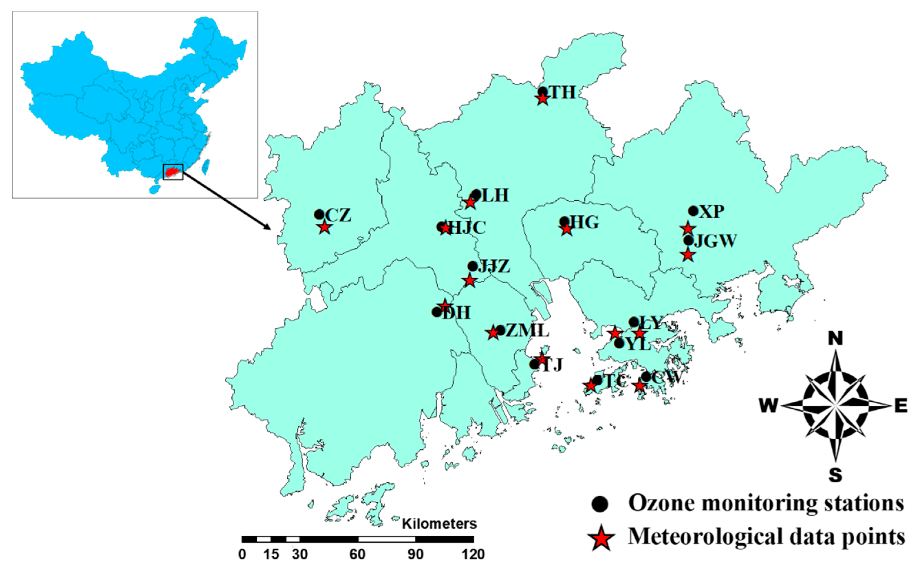
2.1. O3 and Meteorological Data Sets

Maximum daily 8-h moving averages (MDA8) were calculated based on hourly O3 monitoring data at 15 monitoring stations across the PRD from 2007 to 2018. Missing data were imputed based on yearly, monthly, weekly, and hourly averages or were replaced by the O3 data from the nearest monitoring station [36]. Data for 4285 days at the 15 stations were included and the geographical distribution of the data is shown in Figure 1. The latitudes/longitudes and the types of functional areas where the stations are located are shown in Table 1. Meteorological data during the same period, including daily maximum 2-m temperature (T, °C), daily minimum relative humidity (RH, %), total net surface solar radiation (SSR, J/m2), and 10-m mean wind speeds (u and v, m/s; the absolute values of u and v indicate wind speeds, with positive and negative u and v values indicating westerly/southerly and easterly/northerly wind directions, respectively) were retrieved from the European Center for Medium-range Weather Forecast (ECMWF) simulations. Spatial and temporal resolutions were 0.125° × 0.125° and 3 h, respectively. The meteorological conditions at each O3 monitoring station are represented by the simulation data at the point closest to the station, as indicated by the red stars in Figure 1.

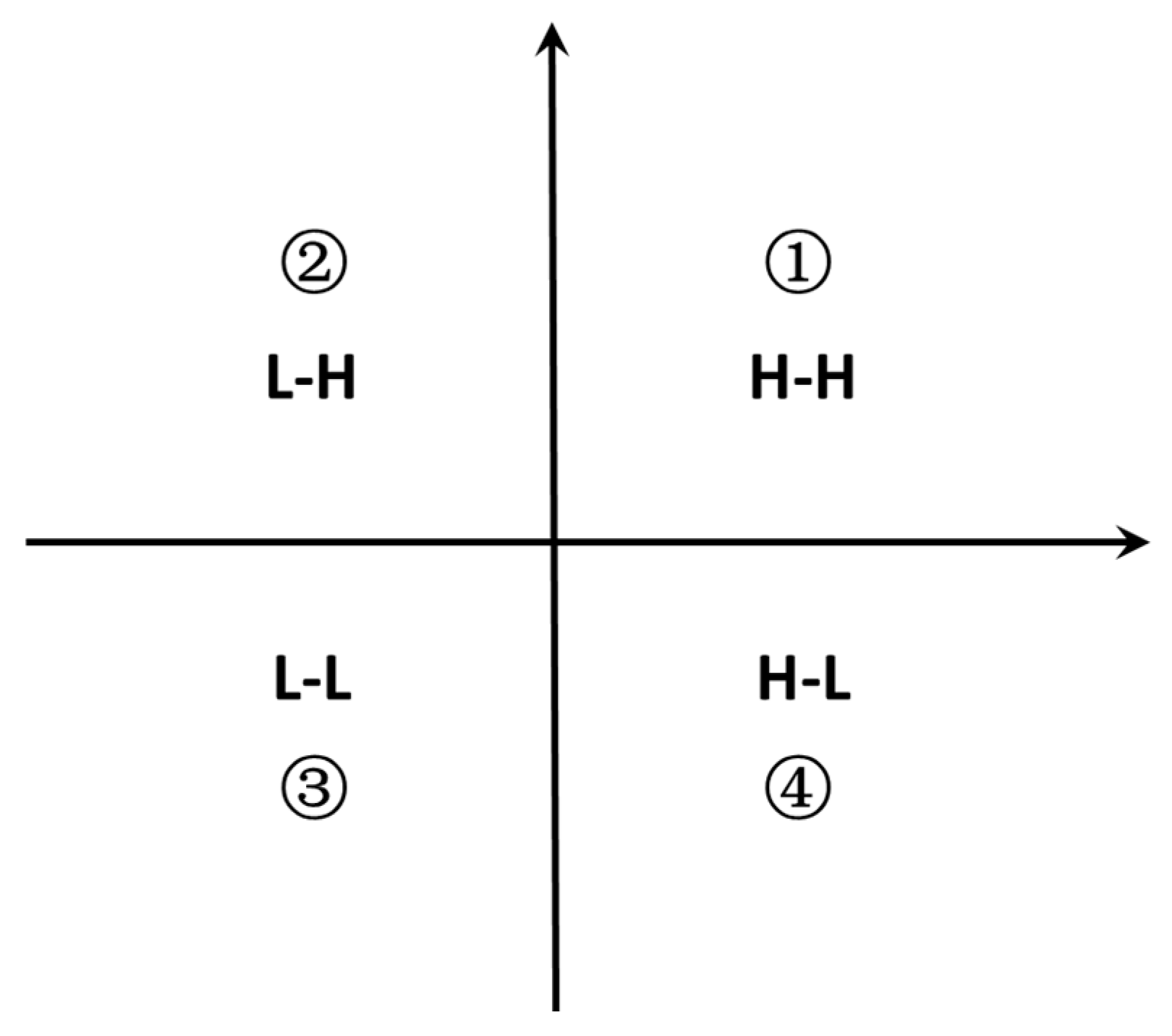
2.2. Identification of the Impacts from Local, Non-Local and Meteorological Factors on O3

To better understand the correlations between O3 and meteorological variables, time (t) data series X(t) were separated into short-term (ST), seasonal (SE), and long-term (LT) components as expressed in Equation (1) [37,38].
X ( t ) = L T ( t ) + S E ( t ) + S T ( t )
The sum of seasonal and long-term trend components is the baseline, and each component can be determined using a KZ filter, which repeats the iterations of a moving average to remove the high-pass signal defined by:
Y i = 1 m j = k k A i + j
where k is the number of values included on each side, the window length m = 2k + 1, i is the interval time, j is the window variables, and Y is the output time series. Different time scales can be obtained by changing the window length and the number of iterations [39,40]. A KZ (15, 5) filter with a window length of 15 with five iterations removes cycles of 33 days referring to the baseline variations (BL).
B L ( t ) = K Z ( 15 ,   5 ) = L T ( t ) + S E ( t ) = K Z ( 365 ,   3 ) + S E ( t )
The long-term trend can be separated from the raw data by KZ (365, 3) with a period >632 days, and then the seasonal and short-term component ST(t) can be derived by
S E ( t ) = K Z ( 15 ,   5 ) K Z ( 365 ,   3 )
S T ( t ) = X ( t ) B L ( t ) = X ( t ) K Z ( 15 ,   5 )
To explore the factors driving the temporal evolution of O3 aggregation and the impacts of meteorological conditions, local and non-local contributions were identified. The methods were as described in our related studies [28]. Briefly, a multiple linear regression (MLP) model was used to perform meteorological adjustments. Local and non-local sources were identified with an empirical orthogonal function (EOF) model and their contributions were estimated with absolute principal component scores (APCS). In our previous investigations, we treated the first principal as non-local, and local contributions were determined by subtracting non-local values from the original data. The statistic models were developed with R language (version 3.5).

2.3. Determination of Relationships between O3 and Meteorological Factors

MLP was conducted using stepwise regression between baseline O3 values and meteorological factors in determining the coefficients of determination [41,42]. We ignored the short-term component as it was weakly correlated compared with the relations between baseline O3 and meteorological variables [35].
A B L ( t ) = a B L + b B L i · M B L i + B L ( t )
where ABL(t) and MBL are the baselines of the O3 and meteorological factors, respectively. The parameters a, b, and are fitted parameters and the residual term. The coefficient of determination (R2) of MLP reflects the relation between O3 and meteorological conditions, and R2 values between O3 and single meteorological factors were obtained if M B L i in Equation (6) contains one meteorological factor. The negative sign will be added to R2 if there exists a negative correlation between O3 and the single meteorological factor.

2.4. Calculation of Degree of Aggregation Dispersion of Stations with Similar O3 Levels

The global Moran’s I index (GM) can be used as a spatial autocorrelation analysis technology to explore the dispersion or unification of attribute values in a given region. In this case, it reflects the correlations of O3 concentrations at different stations, taking the spatial weights of all stations into account. GM values range from −1 to 1, with positive/negative values indicating positive/negative correlations among all O3 stations. GM values approaching 1 or −1 represent strong positive or negative relations, respectively, and a GM value approaching 0 indicates no obvious association. GM was calculated as follows.
I = i = 1 n j = i n w i j ( x i x ¯ ) ( x j x ¯ ) S i = 1 n j = i n w i j
S = 1 n ( x i x ¯ ) 2
x ¯ = 1 n i = 1 n x i
where I is GM, xj is the observed value of a region, wij is the spatial weight matrix, and S is variance. We utilized local Moran’I (LM) to explore the correlation of a station with its adjacent stations in a small area. LM constitutes the normalized O3 concentration of a station and the adjacent station and their scatter plots in quadrant can discern their correlations. It exposes the heterogeneity shadowed by GM and is often involved in recognizing pollution hotspots in geography [43,44,45]. Three stations closest to a site were used to calculate the normalized lagged O3 concentration, which represents the average O3 level adjacent to a site. The normalized O3 value of a site and its lagged value were assigned to a two-dimensional plot and correlations between the two were visualized according to their locations in quadrants (Figure 2). “high-high” (H-H) in the first quadrant [(1) in Figure 2] indicates a site with a high attribute that is encircled by high-attribute sites. Low-high (L-H) in the second quadrant, low-low (L-L) in the third quadrant, and high-low (H-L) in the fourth quadrant indicate a low-attribute site encircled by high-attribute sites, a low-attribute site encircled by low-attribute sites, and a high-attribute site encircled by low-attribute sites, respectively. GM values varied from −1 to +1, with values closer to 1 indicating more strongly positive correlations, which are deemed H-H or L-L patterns, values closer to -1 indicating negative correlations among stations, which are deemed H-L or L-H patterns, and values closer to 0 indicating weaker correlations among stations.

3. Results

3.1. Aggregation of Stations with Similar O3 Concentrations over Different Time Scales

O3 is a regional pollution issue with stations showing similar concentrations distributed close together. The concentration is always affected by meteorological conditions, local precursor emissions and transport of non-local O3 or precursors from outside the local area. The heterogeneity or consistency of average O3 concentrations at multiple stations may vary with changes in these factors, causing fluctuations in the correlations between each station and its adjacent stations. In this section, the aggregation on different time scales, long-term evolution, and driving factors are analyzed to explore the pollution characteristics.

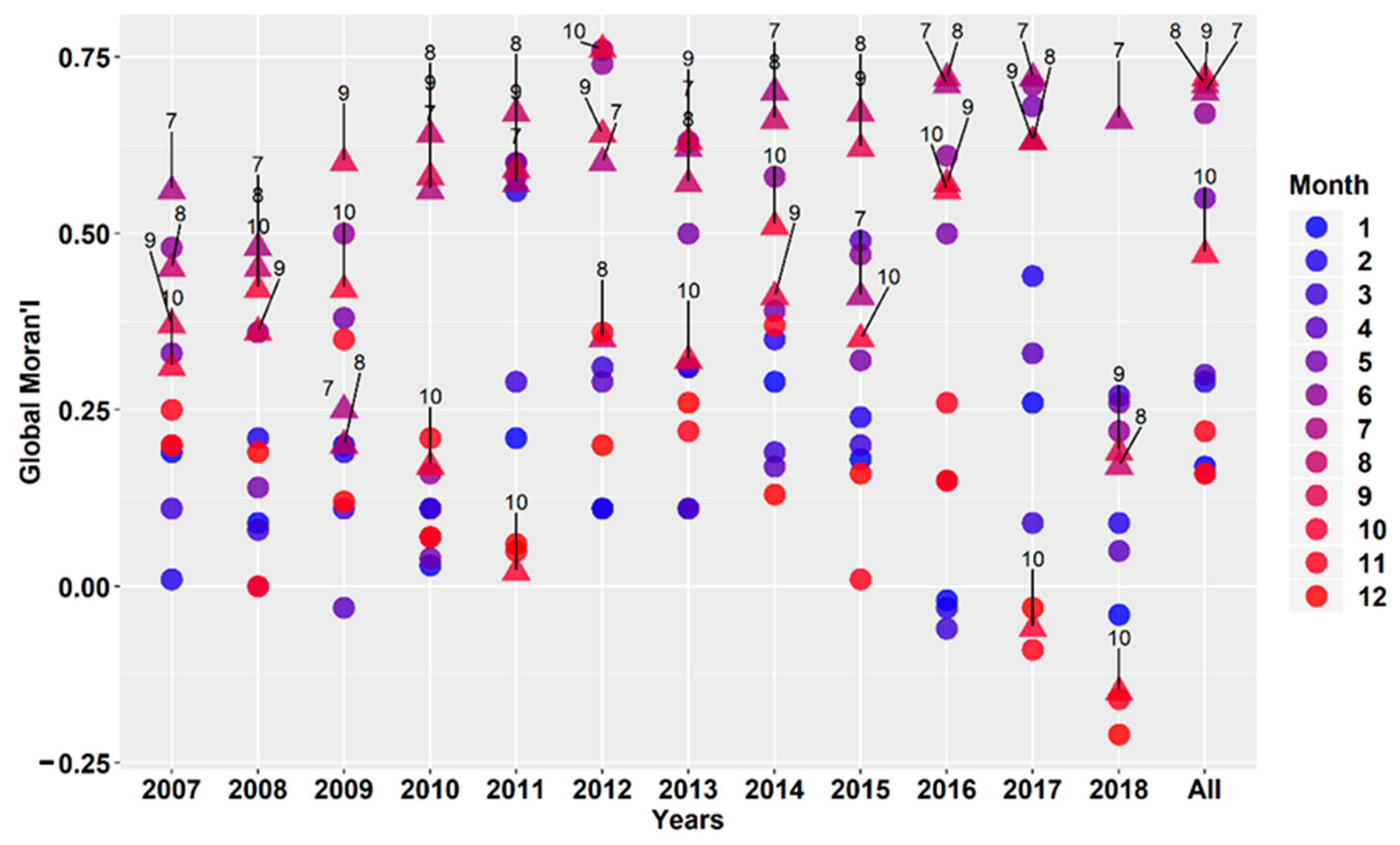
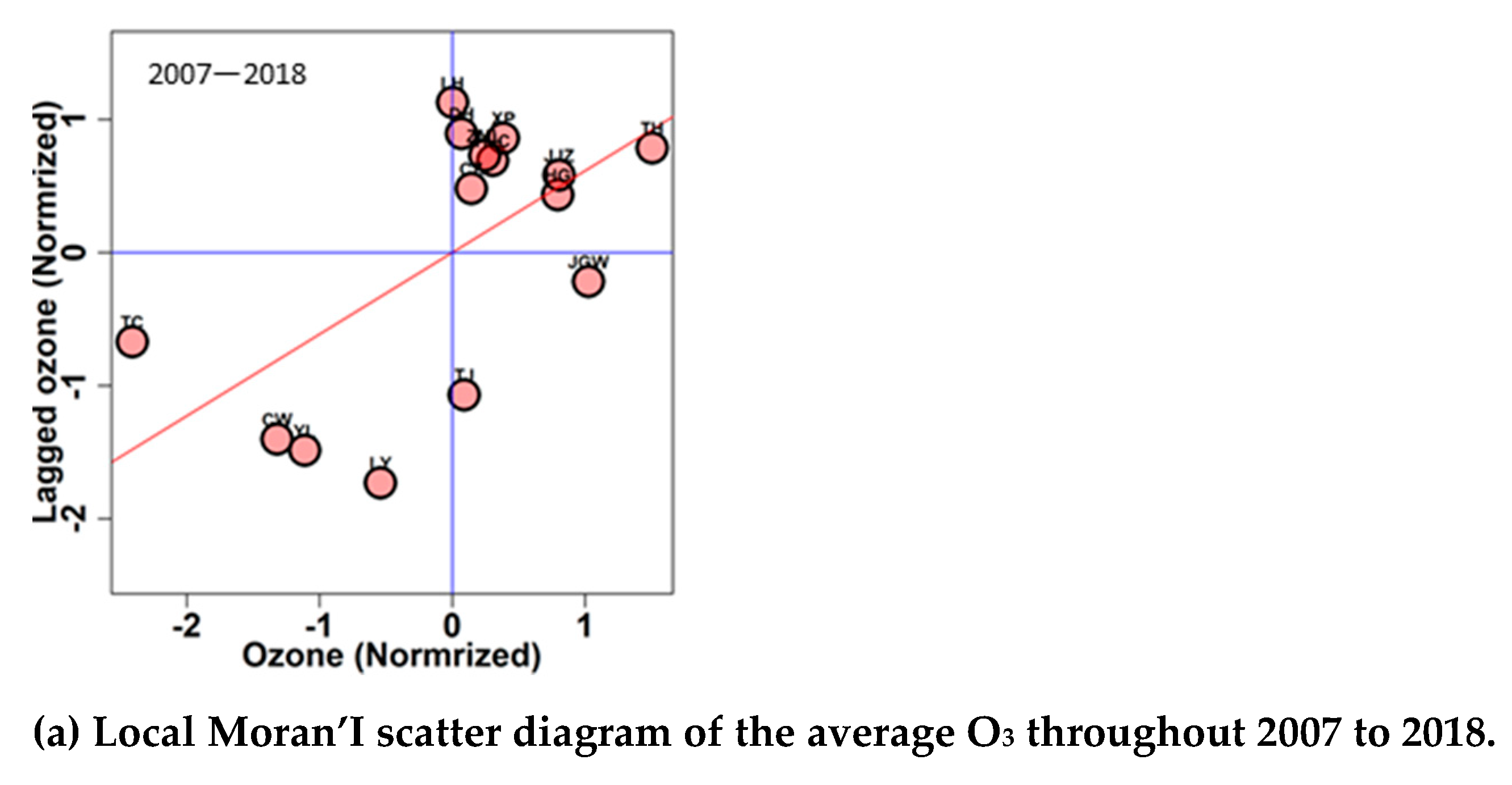
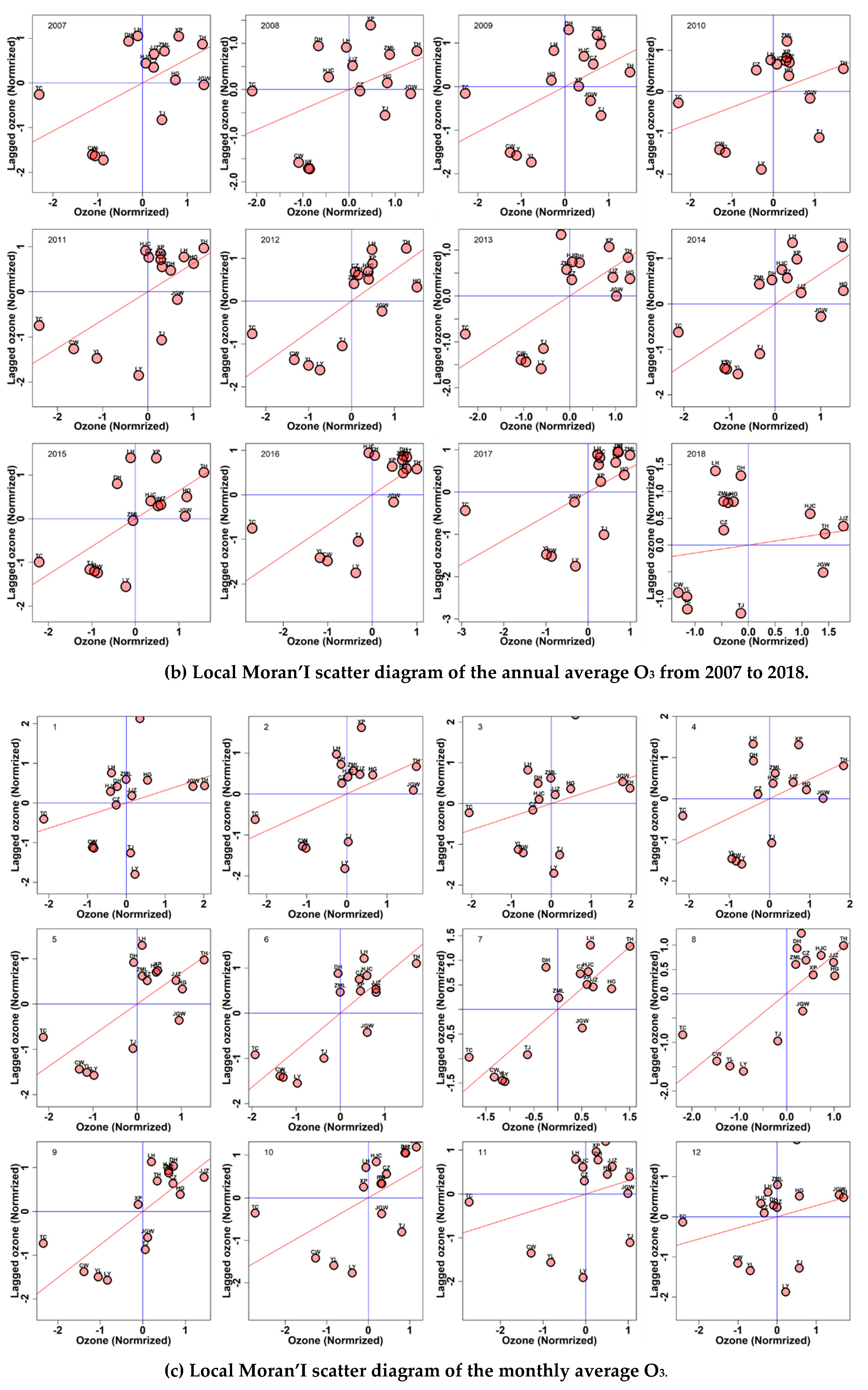
3.1.1. Global Moran’s I on Different Time Scales

GM variations in annual average O3 concentrations are shown in Figure 3 (black line). The values range from a minimum of 0.25 in 2008 to a maximum of 0.59 in 2012 (p < 0.05 except 2018). The positive GM values indicate that stations with similar O3 concentrations distributed agminated in the PRD. The sharp increase from 2007 to 2012 implies that O3 concentrations converged on similar levels during this period and the almost constant GM during the period 2013 to 2017 indicates that the overall spatial distribution of annual average O3 values remained stable throughout the area.
To clarify the factors that drive annual GM values, the impacts of meteorological conditions and local and non-local contributions were identified and their annual GM values are shown in Figure 3. We found that GM values were almost constant regardless of fluctuations in meteorological conditions. This implies that the annual average spatial distribution of O3 is independent of fluctuations in meteorological conditions. Our previous investigation demonstrated that O3 concentrations were sensitive to meteorological conditions in the western region of the PRD [28], while O3 concentrations were high in the northeastern region during the period 2013 to 2017 [46]. Meteorological conditions still have an important influence on O3 concentrations, and we discuss the spatiotemporal evolution of the correlation between O3 and meteorological conditions in Section 3.2.
The annual GM (red line, local GM) decreased when non-local contributions were removed and the annul non-local GM retained the same negative values. Therefore, we inferred that the overall temporal GM was likely driven by local contributions as local and annual GM showed similar temporal variations. Negative non-local GM values near 0 imply that O3 transported from outside of the area was distributed discretely in the PRD. GM values would be increased by the impact of non-local contributions as the discrepancies between O3 concentrations at different stations were evened out by non-local contributions. These observations emphasize that O3 pollution is a regional issue and was intensified by local contributions from 2007 to 2012. Furthermore, O3 concentrations at most stations in the PRD increased during this period [28], and the increasing GM values imply that O3 levels increased faster at stations with previously low levels, thereby reducing the difference compared to high O3 stations. Non-local contributions had no effect on temporal GM fluctuations, whereas they enhanced O3 concentrations at low-level stations. Therefore, local and regional cooperation is necessary to restrict O3 pollution.
It should be noted that GM dropped to 0.1 (p > 0.05) in 2018, implying that O3 concentrations were discretely distributed, which may have been related to abnormal weather in that year. Fluctuations in T and SSR intensified, accompanied by significant differences in temperature and precipitation compared to previous years, and there were several typhoons in 2018 [47]. Different stations were affected to varying degrees by meteorological conditions, resulting stations in high/low O3 levels encompassed by low/high levels stations, which should be explored further in future studies.
Analysis of the monthly GM values for each year compared with the averages of all years (Figure 4) revealed that months with high O3 levels (marked with digits) were usually coupled with high GM values, indicating that O3 concentrations at most stations throughout the region became more similar in O3 seasons. GM values were low or even negative in months with low O3 concentrations. The polarization of GM values in different months demonstrates that control of O3 during periods of high pollution requires the cooperation of the whole area, and appropriate measures should be applied to stations with relatively high O3 concentrations when concentrations are low during spring and winter.

3.1.2. GM on Different Time Scales

GM reflects the autocorrelation of the O3 concentrations of all stations using a single index. This index indicates only the degree of aggregation or dispersion of O3 concentrations in the region. However, heterogeneity between a single station and its adjacent regions within a small district will be shadowed by GM values. Hence, local autocorrelation analysis was performed to examine these features. As shown in Figure 5a, stations were distributed mainly in the first and third quadrants, indicating that stations were surrounded by other stations with similar O3 levels, consistent with high positive GM values. CW, TC, TL, and LY with low concentration levels located in or near Hong Kong (HK) are associated with the L-L pattern because of their relatively low precursor emissions [19]. Furthermore, dilution by the sea breeze and increased precipitation in coastal regions would also lead to low O3 levels in these areas. The remaining stations mostly fell within the first quadrant, indicating that these stations simultaneously experienced high O3 levels compared with those of sites in or near HK. O3 values were highest at TH, and the three nearest stations, HG, HJC, and LH, had similarly high values. These sites are located in the north of the PRD and in northerly winds are the most susceptible to non-local O3 from inland. With a southerly wind, O3 from the south will settle in areas to the north. Both situations could facilitate the accumulation of O3 in areas north of the PRD. JGW and TJ were distributed in the fourth quadrant because of the influence of nearby HK, which had the lowest O3 concentrations. Therefore, programs to restrain O3 in the PRD should take into account geographical location and the effects on upwind areas.
Variations in the scatter diagram of LM for the different years are shown in Figure 5b. Hong Kong remained L-L and most other regions stabilized in the first quadrant throughout the investigation. However, although some stations, such as LH and DH, switched among different quadrants, they finally settled in the first or second quadrant, indicating that these stations coexisted with surrounding high O3 regions. The pattern of GM values in 2018 differed significantly from previous years, which is consistent with the low GM values shown in Figure 3. O3 concentrations at TH, HJC, and JJZ were still relatively high and these stations remained in the first quadrant, while O3 concentrations in other regions were relatively low and switched to the second quadrant. These observations may have been related to abnormal meteorological events in 2018 and require further investigation.
To explore the monthly aggregation in local areas as part of the whole region, we calculated the lagged O3 levels of all stations with the monthly averages from all periods and the results are shown in Figure 5c. The stations were allocated to the quadrants from January to April and during December. This was consistent with the monthly GM values, which were low during the same periods (Figure 4). High O3 concentrations occurred from May to November in the PRD with high monthly GM values (Figure 4) and with monthly local autocorrelations having H-H and L-L patterns (Figure 5c). These observations show that the discrepancies of O3 concentration from the whole region were shrank in high O3 level months, which implied high/low O3 stations were enclosed with high/low stations around during high pollution periods. Inversely, high/low O3 stations were encircled by low/high stations around during non-high pollution periods relatively. These observations indicate the need to formulate different O3 control measures according to specific local pollution conditions.

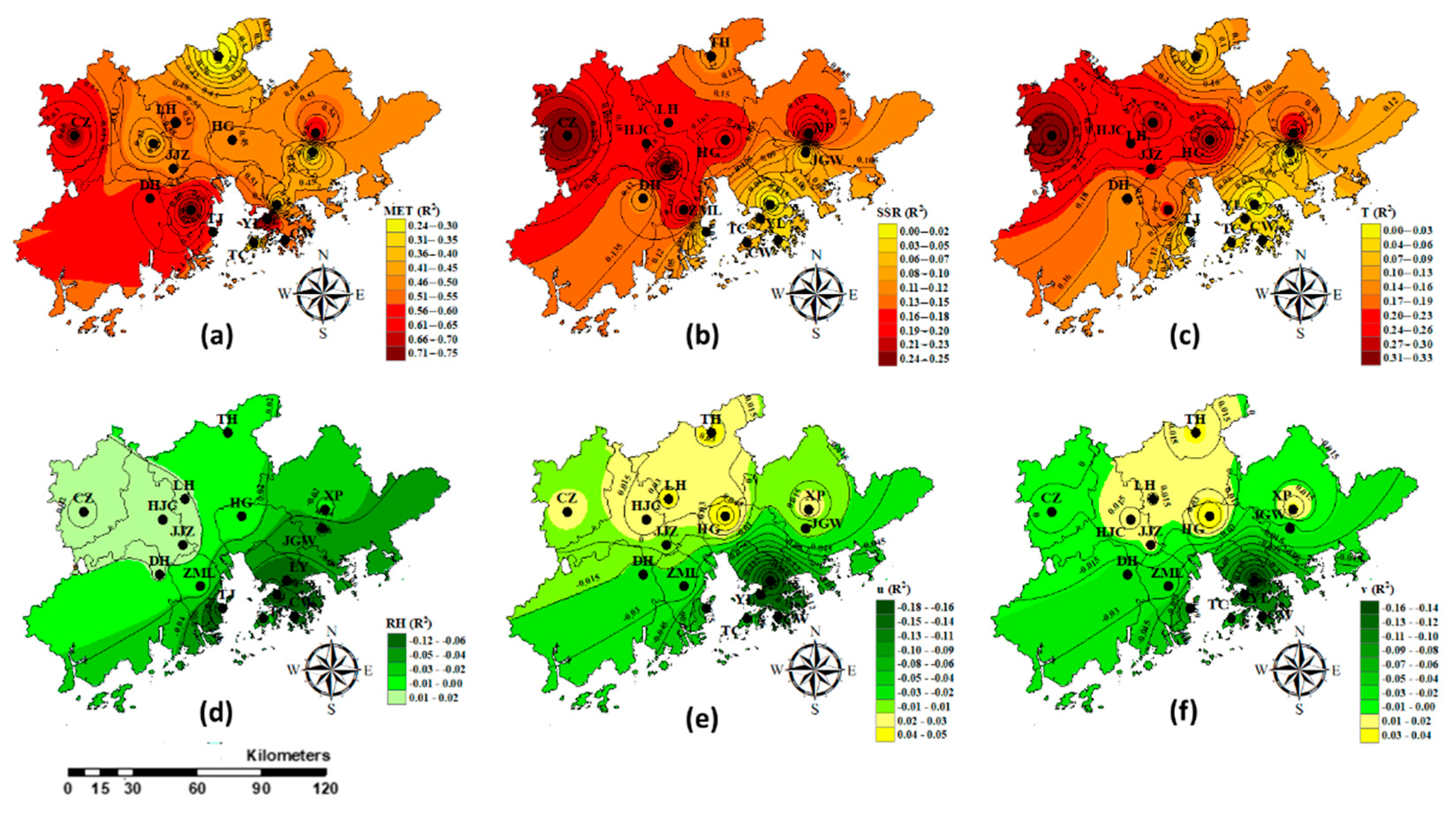
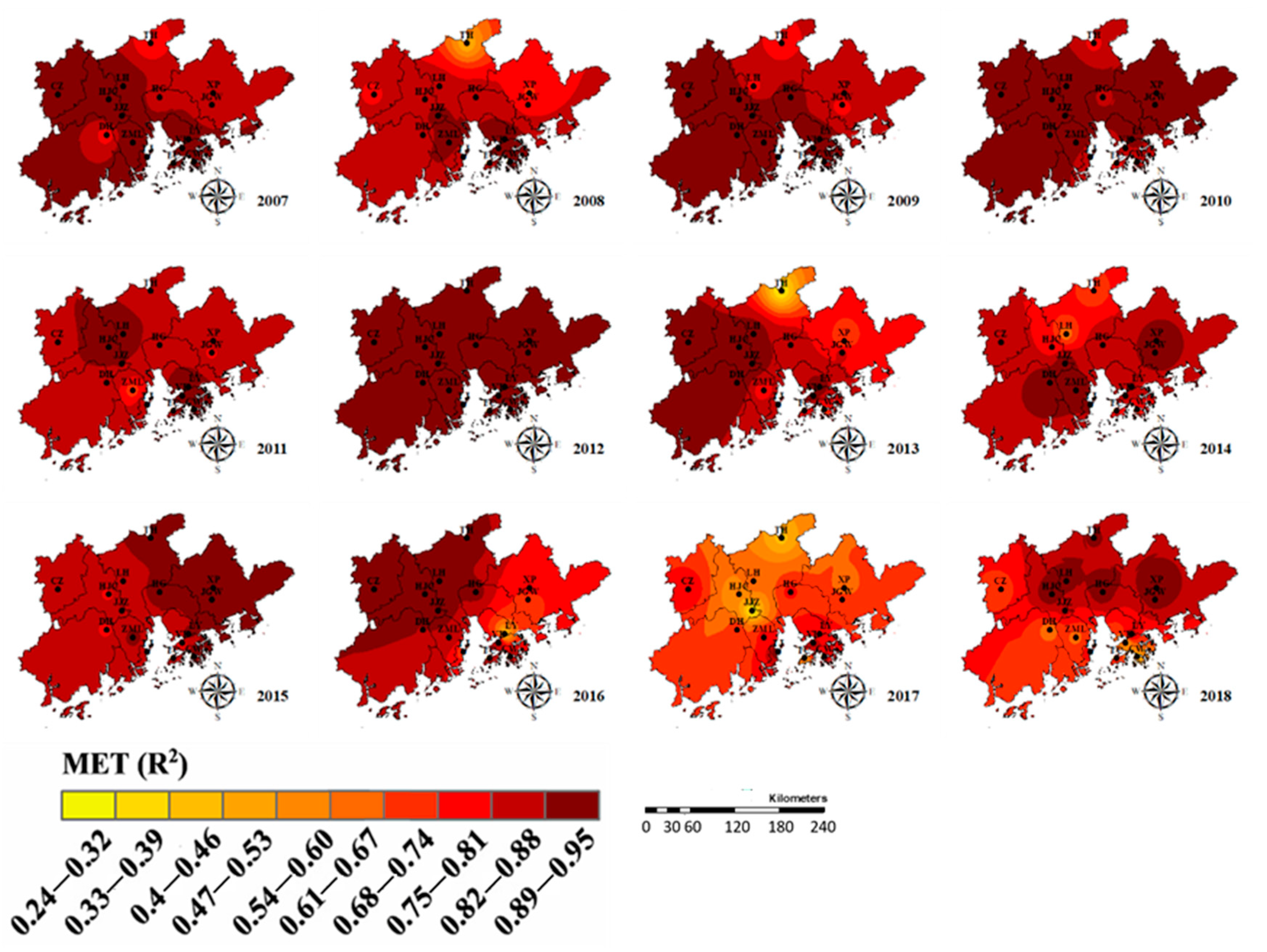
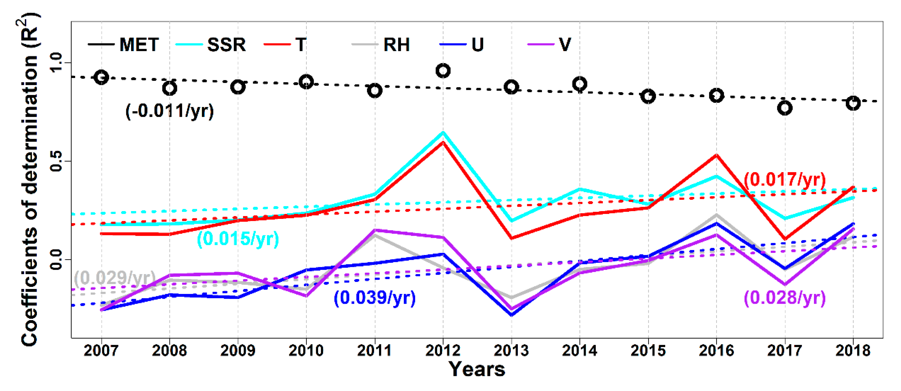
3.2. Spatial Distribution of Meteorological Conditions-O3 Correlations and Its Temporal Evolutionary Characteristics

The results outlined in Section 2 indicate that annual GM values were independent of meteorological conditions. However, O3 concentrations have been shown to be markedly influenced by meteorological fluctuations [29,48,49,50,51,52]. This section discusses the correlation between meteorological fluctuations and their spatiotemporal evolution. As shown in Figure 6a, the R2 values between O3 values and all of the selected meteorological variables (MET) were high throughout the period 2007 to 2018 in southwestern regions and low in northeastern regions, with maximum values of 0.74, 0.72, and 0.67 at YL, CZ, and ZML, respectively. Such high correlations indicate the consistency of variations in O3 concentrations and meteorological conditions and the southwestern region is likely sensitive to meteorological conditions [32,33,34]. R2 values in the northeastern region were relatively low, with a minimum value of 0.24 at TH (Figure 6a), indicating that O3 in these areas was likely regulated mainly by changes in its precursors or by non-local transportation.
R2 values between O3 and single meteorological variables are shown in Figure 6b–f. The R2 of SSR and T (b and c) had similar spatial distributions and governed the overall picture of MET R2, implying that they were the major factors influencing O3 concentrations. R2 values were low in coastal regions, but high in western and central-western areas. This was because precursor emissions of O3 were concentrated in the western and central-western areas [36], and temperature and solar radiation can influence O3 production directly or indirectly. Areas with high precursor emissions are more sensitive to T and SSR and will probably experience higher O3 levels as T and SSR will increase with climate change and with the alleviation of particulate matter pollution. RH showed slight negative correlations in most areas, especially in coastal cities (Figure 6d), which was likely associated with wet deposition of O3 precursors. The R2 values of u and v (Figure 6e–f) had similar spatial distributions and magnitudes, and the negative correlations near the ocean were probably associated with dilution by sea breeze. We speculate that the positive R2 values in the north reflect transport of O3 and its precursors from inland.
The annual geographical distributions and average annual variations in R2 between O3 and all meteorological factors are shown in Figure 7 and Figure 8. High correlations were seen in the southwest in most years, but there were large discrepancies between different years (Figure 7). In the long term, the variations in R2 showed no obvious tendencies for the whole region, except that R2 was relatively low from 2016 to 2018. Examination of the spatial distribution of R2 for each meteorological variable with O3 (Figures S1–S5) implied that the sensitivity of the western area to meteorological conditions was due mainly to SSR and T and that u and v were responsible for the totally high R2 values in the northeast from 2015. R2 values in SSR and T had similar spatial distributions throughout all periods and were higher during the last 8 years than the first few years. Negative correlations were seen between O3 and RH in most periods, especially in coastal areas. The R2 values of u and v with O3 were positive in the north and became more intense with the years, signifying that ozone was more sensitive to wind in the north, while values were negative in the south and the last to become positive, signifying that O3 in the south was likely induced by wind.
Annual MET R2 (black dashed line in Figure 8) values showed a slight decrease from 2007 to 2018, accompanied by increases in R2 values for SSR and T and reductions in RH, u, and v. Hence, MET R2 was suppressed by RH, u, and v overall. R2 values for SSR and T remained highly consistent in tendency and magnitude due to the high correlation between SSR and T. The decline in NOx and increase in VOCs were relatively steady over the last decade [1], so the peaks in 2012 and 2016 were probably related to the marked fluctuations in SSR and T (Figure S6). The increases in R2 values for T and SSR imply that the PRD, especially the areas with O3 concentration sensitive to meteorological conditions, will likely suffer more severe O3 pollution in the future at present emission levels. On the whole, u, v, and RH acted as diluters initially based on the negative R2, and this occurred mainly in the southern parts of the PRD; O3 showed positive correlations with u and v, and was independent of RH in the last few years. Xue et al. reported that Hong Kong was experiencing increasing O3 transport from the PRD [53]. Therefore, we assume that the negative correlations of u-R2 and v-R2 values occurred when dilution by wind was dominant, and O3 concentrations in the PRD were relatively low. More O3 was transported to the south from the PRD when O3 levels in the PRD were high, leading to positive u and v R2 values in the southern regions of the PRD. These findings imply that efforts to reduce emissions may be offset by adverse meteorological conditions and indicate that it is necessary to clarify O3 transport by the wind to restrict levels in the PRD.

4. Conclusions and Discussion

In this study, the aggregation (as reflected by GM) of O3 concentrations at all stations in the PRD and their temporal evolution were analyzed to elucidate regional issues related to O3 pollution. The impacts of meteorology, local and non-local contribution were identified to determine the driving factors of GM variation. The results show that stations with similar O3 levels aggregated distributed more in PRD. The increases in annual GM from 2007 to 2012 indicate that the differences in O3 concentrations among stations decreased and O3 approached to a similar level. Further investigation showed that GM values were independent of meteorological conditions and were markedly enhanced by non-local contributions and that the temporal variations in GM were driven by local contributions. GM values were higher in O3 seasons and became small in low O3 months. Furthermore, stations near HK had similarly low levels and the remainder had high O3 levels, as characterized by LM. Thus, regional O3 issues became more prominent, which was mainly due to local and non-local contributions.
To reduce O3 pollution in the PRD, further substantial reductions in emissions are required. Cooperation between regions within the PRD and with environmental agencies outside the PRD will be crucial to reduce transport from upwind areas. Ozone concentration in the westerly of PRD was more sensitive to T and SSR, and the R2 between ozone and meteorological factors increased over the years, so O3 concentrations will probably increase even if emissions are kept constant as the warming climate, and additional efforts are required to reduce pollution in these areas. Particularly, RH-R2 values were negative in most areas and periods, which is reasonable due to wet deposition in O3 and its precursors. The R2 values of u and v were positive in northern regions and increased over the years, while being negative in southern regions and eventually becoming positive, implying that O3 was more likely to be transported into the area by wind, especially in the northern regions of the PRD. Therefore, it is necessary to characterize the impacts of meteorological conditions for effective emission reduction, and additional attention and efforts are needed in the meteorology-sensitive regions.

Supplementary Materials

The following are available online at https://www.mdpi.com/2073-4433/12/2/279/s1, Figure S1: Annual coefficients of determination (R2) between the baseline of daily MDA8 and SSR. Figure S2: Annual coefficients of determination (R2) between the baseline of daily MDA8 and T. Figure S3: Annual coefficients of determination (R2) between the baseline of daily MDA8 and RH. Figure S4: Annual coefficients of determination (R2) between the baseline of daily MDA8 and u. Figure S5: Annual coefficients of determination (R2) between the baseline of daily MDA8 and v. Figure S6: Annual variances of each meteorological variable.

Author Contributions

Conceptualization, L.Y. and Z.Y.; Data curation, Z.Y.; Formal analysis, L.Y., Z.Y., Z.H., H.W. and J.H.; Methodology, L.Y. and W.J.; Project administration, D.X.; Software, H.W.; Supervision, Z.Y.; Validation, Z.H., J.H. and L.L.; Visualization, L.Y.; Writing—original draft, L.Y.; Writing—review & editing, Z.Y. All authors have read and agreed to the published version of the manuscript.

Funding

This work is supported by National Key Research and Development Project of China (No. 2018YFC1801602).

Institutional Review Board Statement

Not applicable.

Informed Consent Statement

Not applicable.

Data Availability Statement

The data sets are from Guangdong Environmental Monitoring Center and Hong Kong Environmental Protection Department in this study.

Acknowledgments

This work is supported by National Key Research and Development Project of China (No. 2018YFC1801602). The authors are grateful to Guangdong Environmental Monitoring Center and Hong Kong Environmental Protection Department for providing ozone monitoring data over the PRD for use in this study.

Conflicts of Interest

The authors declare that they have no known competing financial interests or personal relationships that could have appeared to influence the work reported in this paper.

References

  1. Bian, Y.; Huang, Z.; Ou, J.; Zhong, Z.; Xu, Y.; Zhang, Z.; Xiao, X.; Ye, X.; Wu, Y.; Yin, X. Evolution of anthropogenic air pollutant emissions in Guangdong Province, China, from 2006 to 2015. Atmos. Chem. Phys. 2019, 19, 11701–11719. [Google Scholar] [CrossRef] [Green Version]
  2. Wang, Y.; Wang, H.; Guo, H.; Lyu, X.; Cheng, H.; Ling, Z.; Louie, P.; Simpson, I.; Meinardi, S.; Blake, D. Long-term O3–precursor relationships in Hong Kong: Field observation and model simulation. Atmos. Chem. Phys. 2017, 17, 10919–10935. [Google Scholar] [CrossRef] [Green Version]
  3. Report on the State of Guangdong Provinccal Environment of 2019. Available online: http://gdee.gd.gov.cn/attachment/0/397/397371/3048134.pdf. (accessed on 17 February 2021).
  4. Stevenson, D.S.; Young, P.J.; Naik, V.; Lamarque, J.; Shindell, D.; Voulgarakis, A.; Skeie, R.; Dalsoren, S.; Myhre, G.; Berntsen, T. Tropospheric ozone changes, radiative forcing and attribution to emissions in the Atmospheric Chemistry and Climate Model Intercomparison Project (ACCMIP). Atmos. Chem. Phys. Discuss. 2013, 13, 3063–3085. [Google Scholar] [CrossRef] [Green Version]
  5. Thompson, A.; Balashov, N.; Witte, J.; Coetzee, J.; Thouret, V.; Posny, F. Tropospheric ozone increases over the southern Africa region: Bellwether for rapid growth in Southern Hemisphere pollution? Atmos. Chem. Phys. 2014, 14, 9855–9869. [Google Scholar] [CrossRef] [Green Version]
  6. Mazzuca, G.; Ren, X.; Loughner, C.; Estes, M.; Crawford, J.; Pickering, K.; Weinheimer, A.; Dickerson, R. Ozone Production and Its Sensitivity to NOx and VOCs: Results from the DIS-COVER-AQ Field Experiment, Houston 2013. Atmos. Chem. Phys. 2016, 16, 14463–14474. [Google Scholar] [CrossRef] [Green Version]
  7. Wang, T.; Xue, L.; Brimblecombe, P.; Lam, Y.; Li, L.; Zhang, L. Ozone pollution in China: A review of concentrations, meteorological influences, chemical precursors, and effects. Sci. Total Environ. 2017, 575, 1582–1596. [Google Scholar] [CrossRef]
  8. Jacob, D.; Horowitz, L.W.; Munger, J.; Heikes, B.G.; Dickerson, R.; Artz, R.; Keene, W.C. Seasonal transition from NOx- to hydrocarbon-limited conditions for ozone production over the eastern United States in September. J. Geophys. Res. Space Phys. 1995, 100, 9315–9324. [Google Scholar] [CrossRef]
  9. Li, L.; An, J.; Shi, Y.; Zhou, M.; Yan, R.; Huang, C.; Wang, H.; Lou, S.; Wang, Q.; Lu, Q.; et al. Source apportionment of surface ozone in the Yangtze River Delta, China in the summer of 2013. Atmos. Environ. 2016, 144, 194–207. [Google Scholar] [CrossRef]
  10. Jin, X.; Holloway, T. Spatial and temporal variability of ozone sensitivity over China observed from the Ozone Monitoring Instrument: Ozone Sensitivity over China. J. Geophys. Res. Atmos. 2015, 120, 7229–7246. [Google Scholar] [CrossRef]
  11. Wu, R.; Xie, S. Spatial Distribution of Ozone Formation in China Derived from Emissions of Speciated Volatile Organic Compounds. Environ. Sci. Technol. 2017, 51, 2574–2583. [Google Scholar] [CrossRef]
  12. Lyu, X.; Liu, M.; Guo, H.; Ling, Z.; Wang, Y.; Louie, P.; Luk, C. Spatiotemporal variation of ozone precursors and ozone formation in Hong Kong: Grid field measurement and modelling study. Sci. Total. Environ. 2016, 569, 1341–1349. [Google Scholar] [CrossRef] [PubMed]
  13. Ye, L.; Wang, X.; Fan, S.; Chen, W.; Chang, M.; Zhou, S.; Wu, Z.; Fan, Q. Photochemical indicators of ozone sensitivity: Application in the Pearl River Delta, China. Front. Environ. Sci. Eng. 2016, 10, 15. [Google Scholar] [CrossRef]
  14. Shao, M.; Zhang, Y.; Zeng, L.; Tang, X.; Zhang, J.; Zhong, L.; Wang, B. Ground-level ozone in the Pearl River Delta and the roles of VOC and NOx in its pro-duction. J. Environ. Manag. 2009, 90, 512–518. [Google Scholar] [CrossRef] [PubMed]
  15. Ou, J.; Yuan, Z.; Zheng, J.; Huang, Z.; Shao, M.; Li, Z.; Huang, X.; Guo, H.; Louie, P.K.K. Ambient Ozone Control in a Photochemically Active Region: Short-Term Despiking or Long-Term Attainment? Environ. Sci. Technol. 2016, 50, 5720–5728. [Google Scholar] [CrossRef] [PubMed]
  16. Wang, N.; Lyu, X.; Deng, X.; Huang, X.; Jiang, F.; Ding, A. Aggravating O3 pollution due to NOx emission control in eastern China. Sci. Total. Environ. 2019, 677, 732–744. [Google Scholar] [CrossRef] [PubMed]
  17. Kuo, Y.; Chiu, C.; Yu, H. Influences of ambient air pollutants and meteorological conditions on ozone variations in Kaohsiung, Taiwan. Stoch. Environ. Res. Risk Assess. 2014, 29, 1037–1050. [Google Scholar] [CrossRef]
  18. Martins, D.; Stauffer, R.; Thompson, A.; Knepp, T.; Pippin, M. Surface ozone at a coastal suburban site in 2009 and 2010: Relationships to chemical and meteorological processes. J. Geophys. Res. Space Phys. 2012, 117, 1156–1163. [Google Scholar] [CrossRef] [Green Version]
  19. Zheng, J.; Shao, M.; Che, W.; Zhang, L.; Zhong, L.; Zhang, Y.; Streets, D. Speciated VOC Emission Inventory and Spatial Patterns of Ozone Formation Potential in the Pearl River Delta, China. Environ. Sci. Technol. 2009, 43, 8580–8586. [Google Scholar] [CrossRef] [PubMed]
  20. Henneman, L.; Shen, H.; Liu, C.; Hu, Y.; Mulholland, J.; Russell, A. Responses in Ozone and Its Production Efficiency Attributable to Recent and Future Emissions Changes in the Eastern United States. Environ. Sci. Technol. 2017, 51, 13797–13805. [Google Scholar] [CrossRef] [PubMed]
  21. Sharma, A.; Ojha, N.; Pozzer, A.; Mar, K.; Beig, G.; Lelieveld, J.; Gunthe, S. WRF-Chem simulated surface ozone over south Asia during the pre-monsoon: Effects of emission inventories and chemical mechanisms. Atmos. Chem. Phys. Discuss. 2017, 17, 14393–14413. [Google Scholar] [CrossRef] [Green Version]
  22. Buysse, C.; Munyan, J.; Bailey, C.; Kotsakis, A.; Sagona, J.; Esperanza, A.; Pusede, S. On the effect of upwind emission controls on ozone in Sequoia National Park. Atmos. Chem. Phys. Discuss. 2018, 18, 17061–17076. [Google Scholar] [CrossRef] [Green Version]
  23. Shu, L.; Wang, T.; Xie, M.; Li, M.; Zhao, M.; Zhang, M.; Zhao, X. Episode study of fine particle and ozone during the CAPUM-YRD over Yangtze River Delta of China: Characteristics and source attribution. Atmos. Environ. 2019, 203, 87–101. [Google Scholar] [CrossRef]
  24. Li, Y.; Lau, K.; Fung, J.H.; Zheng, J.; Zhong, L.; Louie, P. Ozone source apportionment (OSAT) to differentiate local regional and super-regional source contributions in the Pearl River Delta region, China. J. Geophys. Res. Atmos. 2012, 117, 1276–1285. [Google Scholar] [CrossRef]
  25. Kemball-Cook, S.; Parrish, D.; Ryerson, T.; Nopmongcol, U.; Johnson, J.; Tai, E.; Yarwood, G. Contributions of regional transport and local sources to ozone exceedances in Houston and Dallas: Comparison of results from a photochemical grid model to aircraft and surface measurements. J. Geophys. Res. Space Phys. 2009, 114, 1354–1362. [Google Scholar] [CrossRef] [Green Version]
  26. Li, Y.; Lau, A.; Fung, J.; Ma, H.; Tse, Y. Systematic evaluation of ozone control policies using an Ozone Source Apportionment method. Atmos. Environ. 2013, 76, 136–146. [Google Scholar] [CrossRef]
  27. Ambrose, J.; Reidmiller, D.; Jaffe, D. Causes of high O in the lower free troposphere over the Pacific Northwest as observed at the Mt. Bachelor Observatory. Atmos. Environ. 2011, 45, 5302–5315. [Google Scholar] [CrossRef]
  28. Yang, L.; Luo, H.; Yuan, Z.; Zheng, J.; Huang, Z.; Li, C.; Lin, X.; Louie, P.; Chen, D.; Bian, Y. Quantitative impacts of meteorology and precursor emission changes on the long-term trend of ambient ozone over the Pearl River Delta, China, and implications for ozone control strategy. Atmos. Chem. Phys. Discuss. 2019, 19, 12901–12916. [Google Scholar] [CrossRef] [Green Version]
  29. Pacifko, F.J. Isoprene emissions and climate. Atmos. Environ. 2009, 43, 6121–6135. [Google Scholar] [CrossRef]
  30. Folberth, G.; Hauglustaine, D.; Lathière, J.; Brocheton, F. Impact of biogenic hydrocarbons on tropospheric chemistry: Results from a global chemistry-climate model. Atmos. Chem. Phys. 2005, 5, 1267–1280. [Google Scholar] [CrossRef]
  31. Cleary, P.; Wooldridge, P.; Millet, D.; McKay, M.; Goldstein, A.; Cohen, R. Observations of total peroxy nitrates and aldehydes: Measurement interpretation and inference of OH radical concentrations. Atmos. Chem. Phys. Discuss. 2007, 7, 1947–1960. [Google Scholar] [CrossRef] [Green Version]
  32. Fu, T.; Zheng, Y.; Paulot, F.; Mao, J.; Yantosca, R.M. Positive but variable sensitivity of August surface ozone to large-scale warming in the southeast United States. Nat. Clim. Chang. 2015, 5, 454–458. [Google Scholar] [CrossRef]
  33. Jia, L.; Xu, Y. Effects of Relative Humidity on Ozone and Secondary Organic Aerosol Formation from the Photooxidation of Benzene and Ethylbenzene. Aerosol Sci. Technol. 2013, 48, 1–12. [Google Scholar] [CrossRef]
  34. Kavassalis, S.C.; Murphy, J.G. Understanding ozone-meteorology correlations: A role for dry deposition. Geophys. Res. Lett. 2017, 44, 2922–2931. [Google Scholar] [CrossRef]
  35. Seo, J.; Youn, D.; Kim, J.; Lee, H. Extensive spatio-temporal analyses of surface ozone and related meteorological variables in South Korea for 1999–2010. Atmos. Chem. Phys. 2013, 14, 1191–1238. [Google Scholar] [CrossRef] [Green Version]
  36. Zheng, J.; Swall, L.; Cox, W.; Davis, J.M. Interannual variation in meteorologically adjusted ozone levels in the eastern United States: A comparison of two approaches. Atmos. Environ. 2007, 41, 705–716. [Google Scholar] [CrossRef]
  37. Rao, S.T.; Zalewsky, E.; Zurbenko, I. Determining Temporal and Spatial Variations in Ozone Air Quality. J. Air Waste Manag. Assoc. 1995, 45, 57–61. [Google Scholar] [CrossRef] [PubMed]
  38. Rao, T.; Zurbenko, G. Detecting and Tracking Changes in Ozone Air Quality. Air Waste 1994, 44, 1089–1092. [Google Scholar] [CrossRef]
  39. Milanchus, M.; Rao, S.; Zurbenko, I. Evaluating the effectiveness of ozone management efforts in the presence of mete-orological variability. J. Air Waste Manag. Assoc. 1998, 48, 201–215. [Google Scholar] [CrossRef] [PubMed]
  40. Eskridge, E.; Ku, Y.; Rao, T.; Porter, S.; Zurbenko, G. Separating Different Scales of Motion in Time Series of Meteorological Variables. Bull. Am. Meteorol. Soc. 1997, 78, 1473–1483. [Google Scholar] [CrossRef]
  41. Flaum, B.; Rao, T.; Zurbenko, G. Moderating the Influence of Meteorological Conditions on Ambient Ozone Concentrations. J. Air Waste Manag. Assoc. 1996, 46, 35–46. [Google Scholar] [CrossRef]
  42. Wise, E.; Comrie, A. Extending the Kolmogorov–Zurbenko Filter: Application to Ozone, Particulate Matter, and Meteor-ological Trends. J. Air Waste Manag. Assoc. 2005, 55, 1208–1216. [Google Scholar] [CrossRef]
  43. Liu, Q.; Xie, W.; Xia, J. Using Semivariogram and Moran’s I Techniques to Evaluate Spatial Distribution of Soil Micro-nutrients. Commun. Soil Sci. Plant Anal. 2013, 44, 1182–1192. [Google Scholar] [CrossRef]
  44. Huo, N.; Li, H.; Sun, F.; Zhou, D.; Li, G. Combining Geostatistics with Moran’s I Analysis for Mapping Soil Heavy Metals in Beijing, China. Int. J. Environ. Res. Public Health 2012, 9, 995–1017. [Google Scholar] [CrossRef] [PubMed] [Green Version]
  45. Zhang, C.; Luo, L.; Xu, W.; Ledwith, V. Use of local Moran’s I and GIS to identify pollution hotspots of Pb in urban soils of Galway, Ireland. Sci. Total. Environ. 2008, 398, 212–221. [Google Scholar] [CrossRef]
  46. Report on the State of Guangdong Provinccal Environment of 2017. Available online: http://gdee.gd.gov.cn/protect/P0201806/P020180620/P020180620631772750308.pdf (accessed on 17 February 2021).
  47. China Meteorological Data Service Center. 2019. Available online: http://data.cma.cn/ (accessed on 17 February 2021).
  48. Sillman, S.; Samson, P. Impact of temperature on oxidant photochemistry in urban, polluted rural and remote environments. J. Geophys. Res. Space Phys. 1995, 100, 11497–11508. [Google Scholar] [CrossRef]
  49. Olszyna, K.; Luria, M.; Meagher, J. The correlation of temperature and rural ozone levels in southeastern U.S.A. Atmos. Environ. 1997, 31, 3011–3022. [Google Scholar] [CrossRef]
  50. Young, C.; Washenfelder, R.; Roberts, J.; Mielke, L.; Osthoff, H.; Tsai, C.; Pikelnaya, O.; Stutz, J.; Veres, P.; Cochran, A.; et al. Vertically Resolved Measurements of Nighttime Radical Reservoirs in Los Angeles and Their Contribution to the Urban Radical Budget. Environ. Sci. Technol. 2012, 46, 10965–10973. [Google Scholar] [CrossRef]
  51. Xiong, J.; Wei, W.; Huang, S.; Zhang, Y. Association between the Emission Rate and Temperature for Chemical Pollutants in Building Materials: General Correlation and Understanding. Environ. Sci. Technol. 2013, 47, 8540–8547. [Google Scholar] [CrossRef]
  52. Ormeño, E.; Gentner, D.; Fares, S.; Karlik, J.; Park, J.; Goldstein, A. Sesquiterpenoid Emissions from Agricultural Crops: Correlations to Monoterpenoid Emissions an–d Leaf Terpene Content. Environ. Sci. Technol. 2010, 44, 3758–3764. [Google Scholar] [CrossRef]
  53. Xue, L.; Wang, T.; Louie, P.; Luk, C.W.; Blake, D.; Xu, Z. Increasing External Effects Negate Local Efforts to Control Ozone Air Pollution: A Case Study of Hong Kong and Implications for Other Chinese Cities. Environ. Sci. Technol. 2014, 48, 10769–10775. [Google Scholar] [CrossRef] [Green Version]
Figure 1. Distribution of O3 monitoring stations and meteorological data points in the Pearl River Delta.
Atmosphere 12 00279 g001
Figure 2. Scatter plots of local Moran’I in quadrants and the significance of correlation of a station with adjacent stations.
Atmosphere 12 00279 g002
Figure 3. Annual Global Moran’I of different components from 2007 to 2018 in PRD. Lines in black, blue, red, and green are the original, meteorologically adjusted, local and nonlocal data, respectively.
Atmosphere 12 00279 g003
Figure 4. Monthly Global Moran’I variations from 2007 to 2018 in PRD. Colorful solid dots indicate different months in each year and digits hanging above the solid dots mark the high O3 concentration months (7–10). “All” is O3 average throughout all the years.
Atmosphere 12 00279 g004
Figure 5. Local Moran’I variations in different time scales (ac) in PRD. a, b and c are local Moran’I of the averages through 2007 to 2018, each year and each month respectively. The horizontal and vertical pink lines specified the 0 location of x and y axises and the y Indicates the normalized ozone concentration.
Atmosphere 12 00279 g005aAtmosphere 12 00279 g005b
Figure 6. Coefficients of determination (R2) between the baseline of Maximum daily 8-h moving averages (MDA8) and baselines of meteorological variables from 2007 to 2018 (af) is R2 between O3 and all the five meteorological factors (MET), total net surface solar radiation (SSR, c), daily maximum 2-m temperature (T, b), daily minimum relative humidity (RH, d), 10-m mean wind (u, e and v, f) respectively).
Atmosphere 12 00279 g006
Figure 7. Interannual temporal and spatial variations of coefficients of determination (R2) between the baseline of MDA8 and baselines of all meteorological variables (SSR, T, RH, u and v) from 2007 to 2018.
Atmosphere 12 00279 g007
Figure 8. Coefficients of determination (R2) between the baseline of daily MDA8 and baselines of meteorological variables from 2007 to 2018 (MET is R2 between O3 and all the five meteorological factors). Annotations in brackets indicate the increased rate of annual R2.
Atmosphere 12 00279 g008
Table 1. Location of fifteen O3 monitoring stations across the Pearl River Delta and their environmental background.
StationFull NameCityLongitude (E)Latitude (N)Environmental Background
CWCentral/WesternHong Kong114.1522.28Residential/Commercial
CZChengzhongZhaoqing112.4723.05Residential/Commercial
DHDonghuJiangmen113.0822.59Urban
HGHaogangDongguan113.7323.03Residential/Commercial
HJCHuijingchengFoshan113.1023.00Residential/Commercial
JGWJinguowanHuizhou114.3822.93Residential
JJZJinjuzuiFoshan113.2622.81Suburban
LHLuhuGuangzhou113.2823.15Urban
LYLiyuanShenzhen114.0922.55Urban
TCTung ChungHong Kong113.9122.27Residential
THTianhuGuangzhou113.6223.65Rural
TJTangjiaZhuhai113.5822.34Commercial/Industrial
XPXiapuHuizhou114.4023.07Commercial
YLYuen LongHong Kong114.0222.44Residential
ZMLZimalingZhongshan113.4022.50Residential/Commercial
Publisher’s Note: MDPI stays neutral with regard to jurisdictional claims in published maps and institutional affiliations.

