Investigating the WRF Temperature and Precipitation Performance Sensitivity to Spatial Resolution over Central Europe

Abstract

The grid size resolution effect on the annual and seasonal simulated mean, maximum and minimum daily temperatures and precipitation is assessed using the Advanced Research Weather Research and Forecasting model (ARW-WRF, hereafter WRF) that dynamically downscales the National Centers for Environmental Prediction’s final (NCEP FNL) Operational Global Analysis data. Simulations were conducted over central Europe for the year 2015 using 36, 12 and 4 km grid resolutions. Evaluation is done using daily E-OBS data. Several performance metrics and the bias adjusted equitable threat score (BAETS) for precipitation are used. Results show that model performance for mean, maximum and minimum temperature improves when increasing the spatial resolution from 36 to 12 km, with no significant added value when further increasing it to 4 km. Model performance for precipitation is slightly worsened when increasing the spatial resolution from 36 to 12 km while further increasing it to 4 km has minor effect. However, simulated and observed precipitation data are in quite good agreement in areas with precipitation rates below 3 mm/day for all three grid resolutions. The annual mean fraction of observed and/or forecast events that were correctly predicted (BAETS), when increasing the grid size resolution from 36 to 12 and 4 km, suggests a slight modification on average over the domain. During summer the model presents significantly lower BAETS skill score compared to the rest of the seasons.

1. Introduction

Earth system models (ESMs) and climate circulation models (GCMs) are still the principal tools of the scientific community for projecting future climate [1,2]. Nonetheless, both are incapable of simulating local scales, as they currently resolve resolutions of approximately 100 km or coarser, while there are many important climate phenomena that occur at spatial scales of less than 10 km (e.g., convective cloud processes, turbulence, wind patterns over complex terrain, sea breeze effects, etc.). In addition, ESMs and GCMs do not satisfactorily represent vegetation variability, complex topography and coastlines, which are significant components of the physical system that govern the climate change signal on a local or regional scale. To cope with these deficiencies, dynamical downscaling techniques have been developed and are currently adopted, for effectively adapting the large-scale projections of the inferred climate components provided by an ESM or a GCM to regional or local scales, through explicitly solving the process-based physical dynamics of the regional climate system at high spatial resolution, when driven by the large-scale low-resolution data of the ESM/GCM [3,4].

Regional climate models (RCMs) are among the most effective tools for dynamically downscaling global climate projections to local scales [5], but their ability to reproduce current climate conditions needs to be evaluated, in the first place, against observations before being used for such studies. This exercise allows the identification of potential inherent drawbacks related to the assumptions being made by the setup of the RCM, the parameterizations used and their associated uncertainties, as well as an extensive evaluation of the RCM ability to reproduce significant climate features over the domain of interest. Two approaches can be adopted in order to assess RCM’s ability to reproduce current climate, either the use of GCM/ESM data or the use of reanalysis data as initial and boundary conditions of the RCM (e.g., [6,7,8]). GCM/ESM data are obtained using current greenhouse gases (GHG) forcings. The first approach is not flawless, given that GCMs are not forced by observed data, therefore possible systematic errors developed by a GCM/ESM may propagate into the RCM outputs. As a result, the added value of an RCM used for downscaling purposes might be diminished. Still, such simulations are very useful, as they allow climate projections and assessments for various climate change scenarios on finer resolutions than those resolved by the GCMs/ESMs. On the other hand, reanalysis data are the most accurate representation of the archived climate observations at high temporal and spatial resolution forced by climatic observation, therefore they are extensively used for evaluation purposes of the current climate.

Among the climatic parameters assessed by RCMs, temperature and precipitation are two parameters of crucial relevance for our societal life and the ecosystems. Being able to correctly capture or project their temporal, spatial and quantitative distribution is of high importance. However, their simulation is still very challenging given the wide range of processes involved. Increasing the spatial resolution resolved by RCMs can, to some extent, address the deficiencies in correctly capturing their temporal, spatial and quantitative distribution when downscaling techniques are applied. Multi-nesting approaches in downscaling procedures can add more detail in the assessments, ensuring at the same time that the outputs at the finer scales resolved by the nests of the RCM are dynamically consistent with the large-scale flows. However, the use of several consecutive nests is both a computationally demanding process and does not assure a perfect replicability, degradation or improvement by the RCM outputs. As a result, a number of studies have been conducted assessing the spatial resolution effect, when multi-nesting approaches are used, on models’ performances.

Long term studies have been conducted over Europe, reaching up to 12 km grid-point distance. Vautard et al. [9] examined heatwave prediction within the EURO-CORDEX project at 50 and 12 km resolutions using a multi-model ensemble. They found that there is no significant improvement in maximum temperature prediction, especially in mountainous regions. Kotlarski et al. [10], within the same framework, examined air temperature and precipitation at grid resolutions of 50 and 12 km and could not find clear benefit by the increase in the grid spacing. This was also the conclusion of Jaeger et al. [11] for temperature and precipitation within the ENSEMBLES project at 0.44° and 0.22° spatial resolutions as well as van Roosmalen et al. [12] for Denmark. However, Heikkilä et al. [13] found noteworthy added value comparing 30 and 10 km simulations over Norway.

A number of studies [14,15,16] focus only on precipitation sensitivity with respect to various spatial resolutions and regions. Their results address the estimated biases which do not seem to be clearly improved. Giorgi and Marinucci [14] found that precipitation amount, intensity, and distribution depend on the grid size. Leung and Qian [15] found that the increase of the resolution (from 40 to 13 km) did not cause a uniform improvement of precipitation assessments over complex terrains. Li et al. [16] found that increasing the horizontal resolution from 30 to 10 km improved the forecasting ability for precipitation. Rauscher et al. [17] in the framework of the ENSEMBLES project found that both patterns and temporal evolution of precipitation during summer are improved when decreasing grid spacing from 50 to 25 km. Chan et al. [18] also found added value in capturing precipitation events in topographically complex regions as a result of decreasing grid spacing. Precipitation spatial pattern representation is improved but only a small or not significant improvement can be detected for mean biases along coastlines [7]. Prein et al. [19] examined the representation of mean and extreme precipitation within the EURO-CORDEX project at 0.44° and 0.11° resolutions and found that increased resolution adds value, while in regions with complex terrain (e.g., Alps, the Carpathian) added value in precipitation biases tends to cancel out by averaging. Similar were the findings of Torma et al. [20] within the EURO-CORDEX framework that found improvement in the spatial representation and the extremes of precipitation at finer grid resolutions.

Despite the large number of studies examining the effect of the spatial resolution on models’ performances, the question of up to what spatial scales downscaling global data to local scales can actually improve local representation of temperature and precipitation and whether very fine resolutions (below 10 km) are necessary for their improved representation still remains inadequately addressed. Addressing this challenge, in this study we assess the Advanced Research Weather Research and Forecasting model (ARW-WRF, hereafter WRF) [21,22] temperature and precipitation performance sensitivity to the grid size resolution. Performance sensitivity is examined for WRF downscaled simulated mean, maximum and minimum daily temperatures as well as precipitation and we compare the model’s predictions against daily data from the E-OBS data base [23], in order to draw conclusions on the added value of their representation in higher grid size resolution scales. The grid size resolutions selected here, i.e., 36, 12, and 4 km, extend beyond the typical size of 0.11° (~12 km) used in previous studies (e.g., [24,25,26]). The selected domain is extended over central Europe, due to the significant number of observational data, for assessing both annual and seasonal impact.

2. Materials and Methods

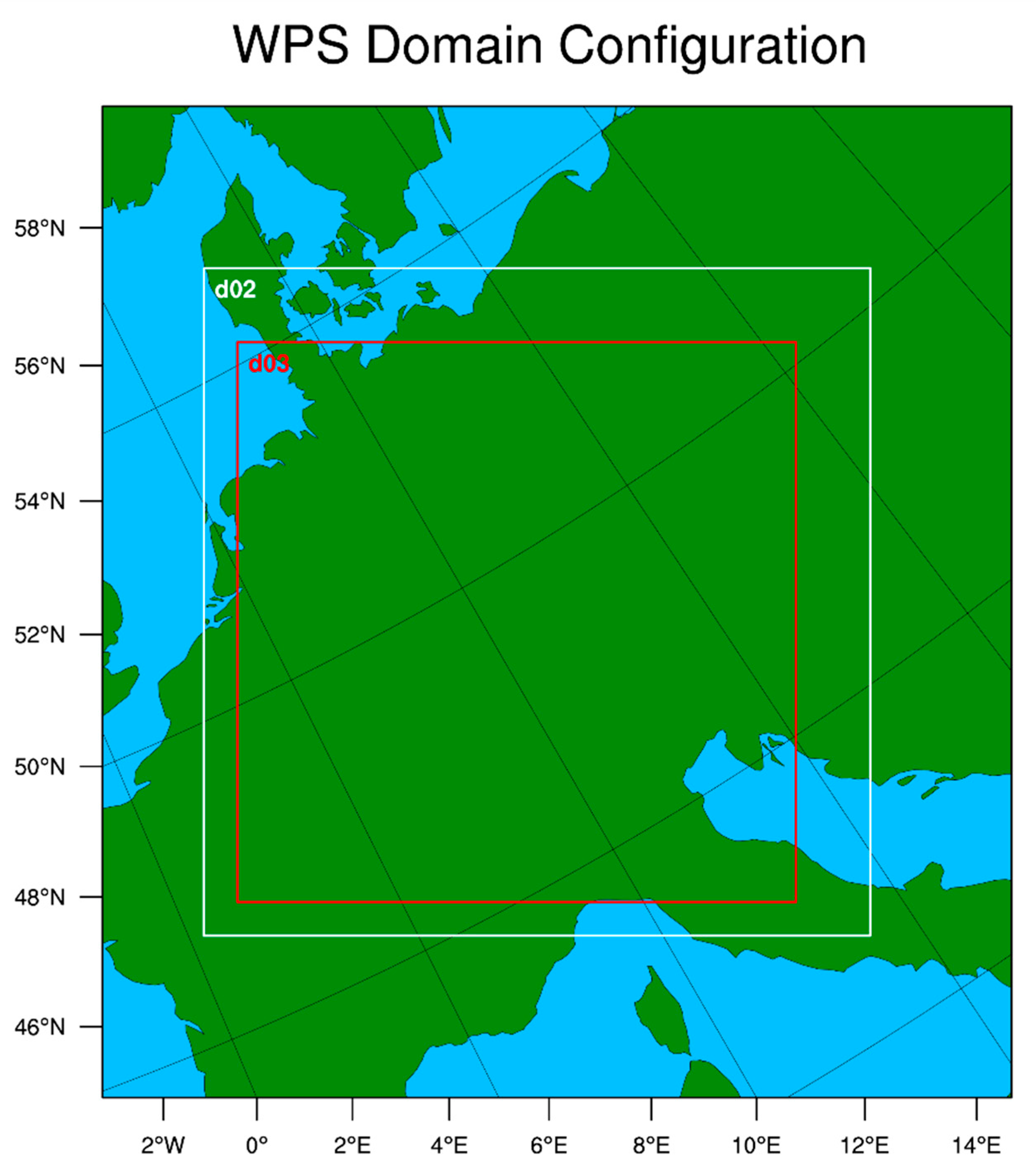
2.1. Modeling Setup

The Weather Research and Forecasting (WRF) model [21,22] version 3.9.1 is used to simulate meteorological variables. WRF is one of the most widely used Regional Climate Models (RCMs) for downscaling global data to regional scales. It is a mesoscale numerical weather prediction system used for reproducing local weather and climate at high spatial resolutions. It has extensively been used for climate and meteorological applications over Europe (e.g., [25,26,27]).

In this study, the parent-coarse model domain is centered at (49°N, 10.5°E) and consists of 50 grid cells east and north with a grid cell size of 36 km. The two nested domains have 100 and 250 grid cells in the west–east and south-north direction with grid cell sizes of 12 and 4 km, respectively. The finer nested domain covers the central European region (Figure 1). The nests are one-way interactive to avoid feedback of the inner to the outer domains so that the results represent the resolution effect only. In the vertical direction, the model used 40 layers. The NCEP FNL (Final) Operational Model Global Tropospheric Analyses data at 1-degree resolution are used as the single initial and lateral boundary conditions for the parent domain, while the latter is updated every 6 hours throughout the model simulations. The modeling setup is similar to the one used in the WRF EURO-CORDEX framework [10,25] for all grid resolutions, employing the WSM-5 microphysics scheme, the RRTMG radiation scheme, the YSU PBL scheme, and the NOAH land surface scheme. Simulations cover the period July 2014 to December 2015, with a 6 month period being used as a spin-up time, allowing a more realistic development of snow cover [28].

2.2. Observational Data

Comparison between predicted and observed values for mean, maximum, minimum temperatures and precipitation is performed for the year 2015 using daily data from the E-OBS dataset [[23,29]. The E-OBS data are based on the European Climate Assessment and Dataset (ECA&D) project station observation data (https://www.ecad.eu/download/ensembles/download.php#datafiles (accessed on 5 February 2021)) that covers the entire European domain. The E-OBS dataset has extensively been used in the past for comparison studies over Europe (e.g., [10,26,30,31,32,33,34,35]). To evaluate model performance, results were compared with the ensemble mean of the regular 0.25° grid version of the E-OBS v20.0e observational dataset. Therefore, the E-OBS grid of 0.25-degree is used as a reference upon which all WRF domain grids are interpolated. After interpolating model-derived temperature, and precipitation to the E-OBS grid within the investigation area, i.e., D3 domain, mean, maximum, minimum temperatures, and precipitation were calculated. One could argue that the specific database is too coarse to compare against the finer domain’s outputs, however, as pointed out by Prein et al, [19] and Fantini et al, [36], it is anticipated that if processes are captured better at higher resolution, improvements are still visible when regridded to coarser resolution. As a result, in order to assure a fair intercomparison among the three grid resolutions, we chose to regrid variables to the grid of E-OBS.

Despite the extensive use of the E-OBS database, there are some known shortfalls related to the spatial coverage of its network stations and the quality of the data where sparse density of stations exist, affecting the magnitude of daily extremes in temperature (e.g., [32,37,38,39,40,41]) and possibly the total precipitation that is underpredicted [41], especially in mountainous and snow-covered regions [42]. However, given that E-OBS has a dense station network with good temporal coverage over central Europe, it has been selected for our study, as its known inefficiencies will not affect the comparison with our simulated data.

2.3. Performance Metrics

Mean bias (MB), separated into positive and negative biases for avoiding any misleading results due to counterbalancing of positive and negative values, mean absolute error (MAE), root mean square error (RMSE) and the index of agreement (IoA) (

Table 1. Statistical Measures.

$\mathrm{Mean}\mathrm{Bias}\left(\mathrm{MB}\right)=\frac{{{\displaystyle \sum }}_{i=1}^n\left(X_{predicted}-X_{observed}\right)}{n}$

$\mathrm{Mean}\mathrm{Absolute}\mathrm{Error}\left(\mathrm{MAE}\right)=\frac{{{\displaystyle \sum }}_{i=1}^n\left|X_{predicted}-X_{observed}\right|}{n}$

$\mathrm{Root}\mathrm{Mean}\mathrm{Square}\mathrm{Error}\left(\mathrm{RMSE}\right)=\sqrt{\frac{{{\displaystyle \sum }}_{i=1}^n{\left(X_{predicted}-X_{observed}\right)}^2}{n}}$

$\mathrm{Index}\mathrm{of}\mathrm{Agreement}\left(\mathrm{IoA}\right)=1-\frac{{{\displaystyle \sum }}_{i=1}^n{\left(X_{predicted}-X_{observed}\right)}^2}{{{\displaystyle \sum }}_{i=1}^n{\left(\left|X_{predicted}-{\overline{X}}_{observed}\right|+\left|X_{observed}-{\overline{X}}_{observed}\right|\right)}^2}$

) are the statistical indices used in order to assess the impact of grid size resolution on the model’s simulated outputs for temperature and precipitation. These metrics are widely used and simply reproducible allowing in a rigorous way the assessment of the model performance. The statistical analysis is based on the daily values for each individual model grid cell assessing both annual and seasonal impacts. In Table 1, X_predicted and X_observed stand for the daily gridded predicted and observed values, with n being the total number of grid points, while overbars denote mean values.

In addition, the bias adjusted equitable threat score (BAETS) [43] for precipitation is used in order to assess how well the forecast “yes” correspond to the observed “yes” events.

Table 2. Contingency table illustrating the counts used for bias adjusted equitable threat score (BAETS) calculation.

		Observed
		Yes	No	Total
Forecast	Yes	Hits (H)	False alarms (Z)	Forecast Yes (F = H + Z)
	No	Misses (Y)	Correct negatives (W)	Forecast No (Y + W)
Total		Observed Yes (O = H + Y)	Observed No (Z + W)	Total (N = H + Z + Y + W)

presents the 2 × 2 contingency table in the form required for this analysis, used in verifying dichotomous forecasts.

The BAETS is given by the formula:

$$BAETS=\frac{H_A-F\frac{O}{N}}{F+O-H_A-F\frac{O}{N}}$$

(1)

where H_A is the bias adjusted number of hits (H),

$$H_A=O-\frac{F-H}{\ln \left(\frac{O}{O-H}\right)}lambertw\left(\frac{O}{F-H}\ln \left(\frac{O}{O-H}\right)\right)$$

(2)

where lambertw stands for the Lambert W-function or omega function, F denotes the forecast event (correctly forecast area or “hits” plus the “false alarms”), O denotes the observed area and N denotes the total number of verification points or events. BAETS has a value between −⅓ and 1, with 0 indicating no skill and 1 is the perfect score.

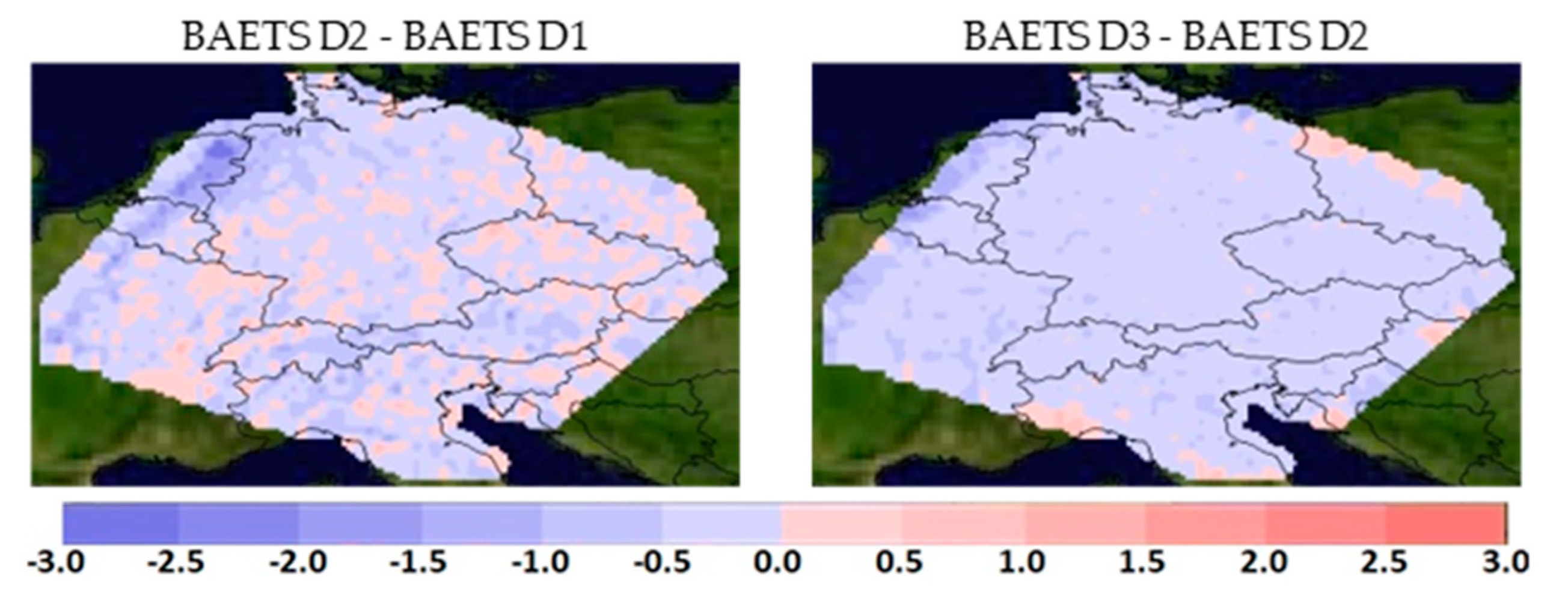
3. Results and Discussion

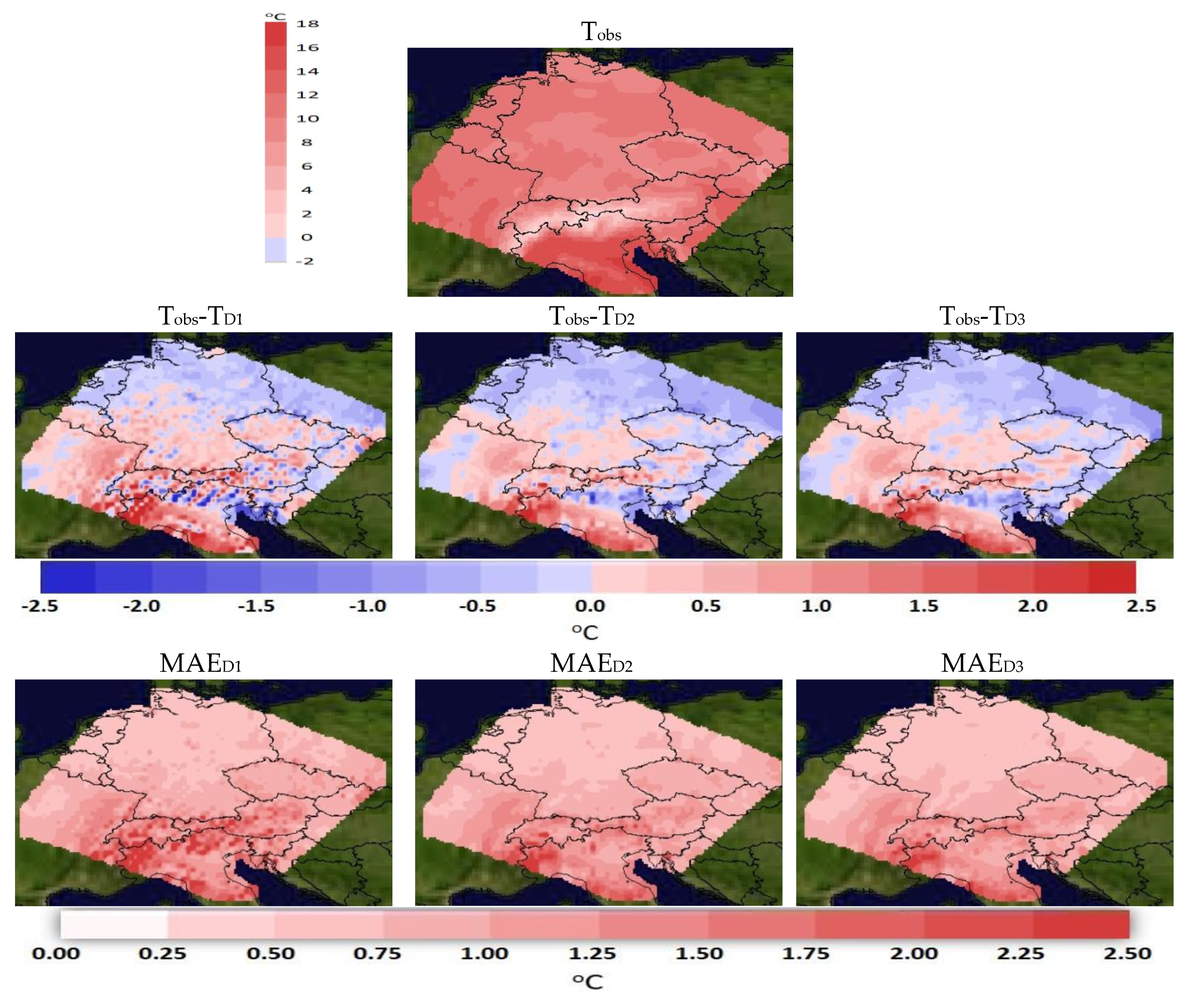
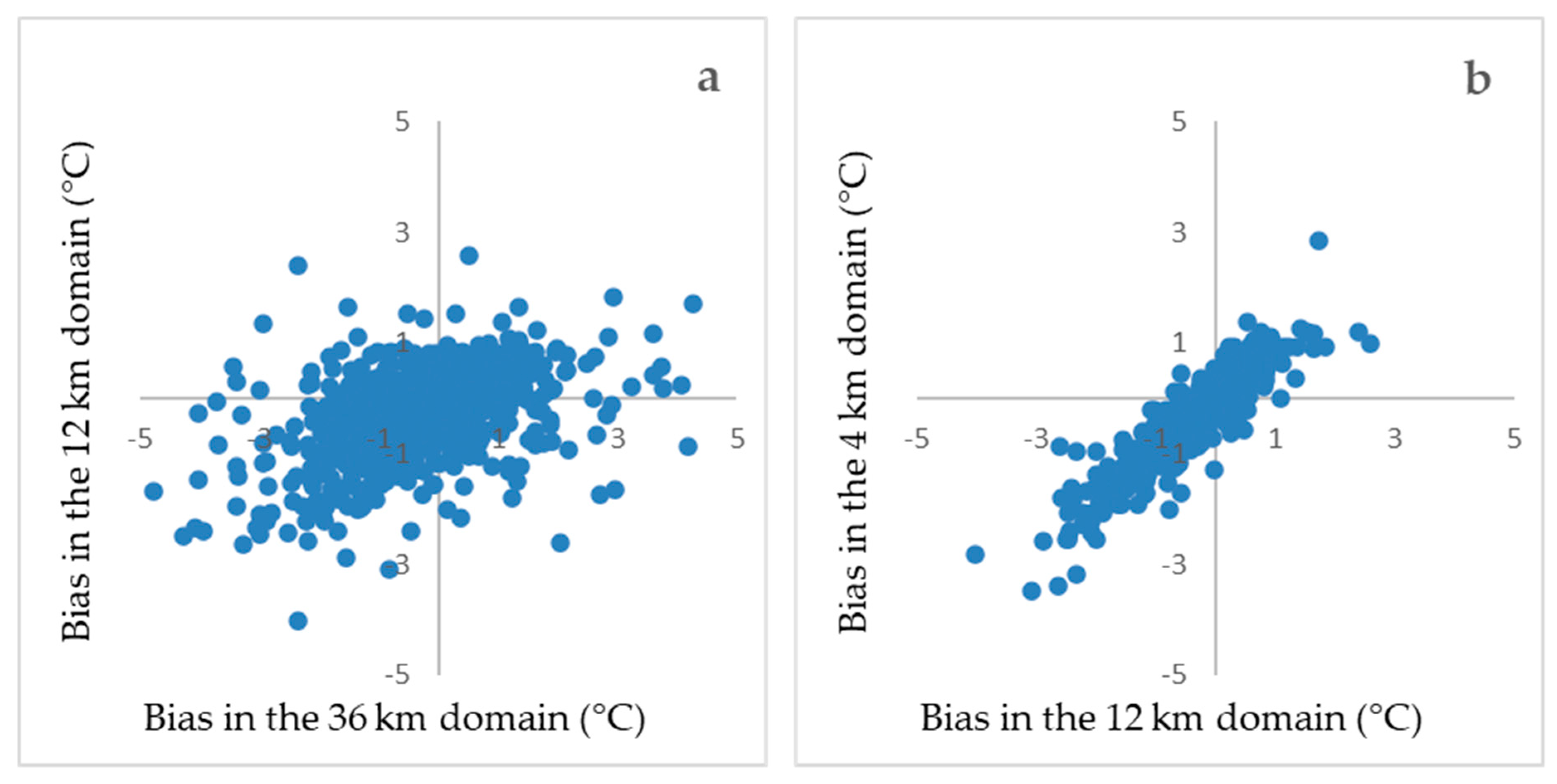
3.1. Mean Temperature

The model reproduces the observed annual domain mean temperature over all three grid size resolutions used in this study. As can be seen in

Table 3. Annual mean temperature statistical analysis (°C).

	D1 (36 km)	D2 (12 km)	D3 (4 km)	Δij (D2-D1)	Δij (D3-D2)
Mean Observed	10.22			-	-
Mean Predicted	10.09	10.10	10.12	-	-
Positive ΜΒ	0.48	0.34	0.32	0.40	0.13
Negative ΜΒ	−0.69	−0.53	−0.52	−0.39	−0.09
RMSE	0.87	0.61	0.59	0.72	0.19
IoA	0.97	0.98	0.99	0.98	1
MAE	0.59	0.44	0.43	0.39	0.10

, there is an average underestimation of the observed mean temperature of 0.13 °C for the 36 km grid size domain (D1), of 0.12 °C on average for the 12 km grid size domain (D2), and of 0.10 °C on average for the 4 km grid size domain (D3). An overestimation is found mainly over the north and northeast region of the domain and an underestimation over the southern part of the domain. This finding, i.e., the cold bias at the north and the warm bias at the south part of Europe has also been stated in other RCM studies [10,26]. The highest positive and negative differences are found in regions characterized by complex orographic features, e.g., the Alps and northern Italy (Figure 2). This trend, as well as the spatial pattern, do not change, in general, with the increase in the spatial resolution. However, model performance is better when decreasing the grid spacing from 36 (D1) to 12 km (D2) but no significant change is found when the spatial resolution is further increased (i.e., 4 km (D3)).

This is also supported by the domain wide average values of the statistical measures for D1-D3 (Table 3). These measures show statistically significant improvement in the biases, the RMSE and the MAE when increasing the spatial resolution from 36 to 12 km, while a minor improvement is seen with further increase of the resolution to 4 km. From a statistical point of view, this implies that simulations with a grid size of 12 km might be adequate to describe annual temperature trends, derived from daily data, over large regions, avoiding computationally demanding simulation with fine grid spacing. Comparing the grid data between domains D1 against D2 and D2 against D3 (Table 3, columns Δ_ij(D2-D1) and Δ_ij(D3-D2)) it is clear that there is a statistically significant change on the average values of biases and RMSE between D1 and D2, and a minor change between D2 and D3 with the reduction of the grid resolution. The better closure between D2 and D3 grid data implies that there is no clear statistical evidence of improvement when downscaling data to the finer grid resolution used here (i.e., 4 km).

Investigating the climatological variability of annual average temperatures in combination with the grid size effect, we compare the grid biases, i.e., simulated minus observed daily values for each grid, for domains D1 against D2 (Figure 3a) and D2 against D3 (Figure 3b). The D2 simulation tends to reduce biases compared to D1 with slightly higher temperatures (below the diagonal). The biases between the D2 and D3 simulations are very similar (mostly fall on the diagonal) and smaller in range than the D1 simulation (Figure 3). As a result, the improvement is higher for D2 compared to D1, with no significant added value being seen for D3 compared to D2.

In addition, the spatial error variability, defined as the difference between the first (25th) and third (75th) quartile, is derived for the three domain resolutions. Results show improvement in the spatial error variability (0.85 °C for D1, 0.70 °C for D2 and 0.68 °C for D3) with the reduction of the grid resolution. Although a clear improvement is seen when comparing D1 against D2, there is no clear evidence of improvement when comparing D2 against D3. These findings also support the conclusion derived from the statistical analysis that simulations with a grid size resolution of 12 km are sufficient for describing annual temperature trends over large domains.

The seasonal mean temperature plots present a similar spatial pattern between the three domains for each season (Figures S1–S4 of Supplementary Material). During autumn, the model, for all grid resolutions, overestimates mean temperature over a major part of the domain and underestimates it mainly over the northwest and central parts of Italy (Figure S1). Increasing the spatial resolution from 36 (D1) to 4 km (D3) improves the statistical metrics (Table S1), suggesting that the finer domain better represents autumn mean temperature. This is related to both the positive and negative MBs which are improved when moving from the coarser to the finer resolution. During winter the model, in all three grid resolutions, underestimates mean temperature mainly over northwest Italy and the region over the Alps (Figure S2). Increasing the spatial resolution from 36 (D1) to 12 km (D2) leads to improved statistical measures (Table S2) but no significant change is found when the spatial resolution is further increased (i.e., 4 km (D3)). During spring and summer, the model, in all grid resolutions, underestimates mean temperature in most parts of the domain with an exception of the north–northeast region (Figures S3 and S4). Increasing the spatial resolution from 36 (D1) to 12 km (D2) leads to improved statistical measures (Tables S3 and S4) but no significant change is found when the spatial resolution is further increased (i.e., 4 km (D3)).

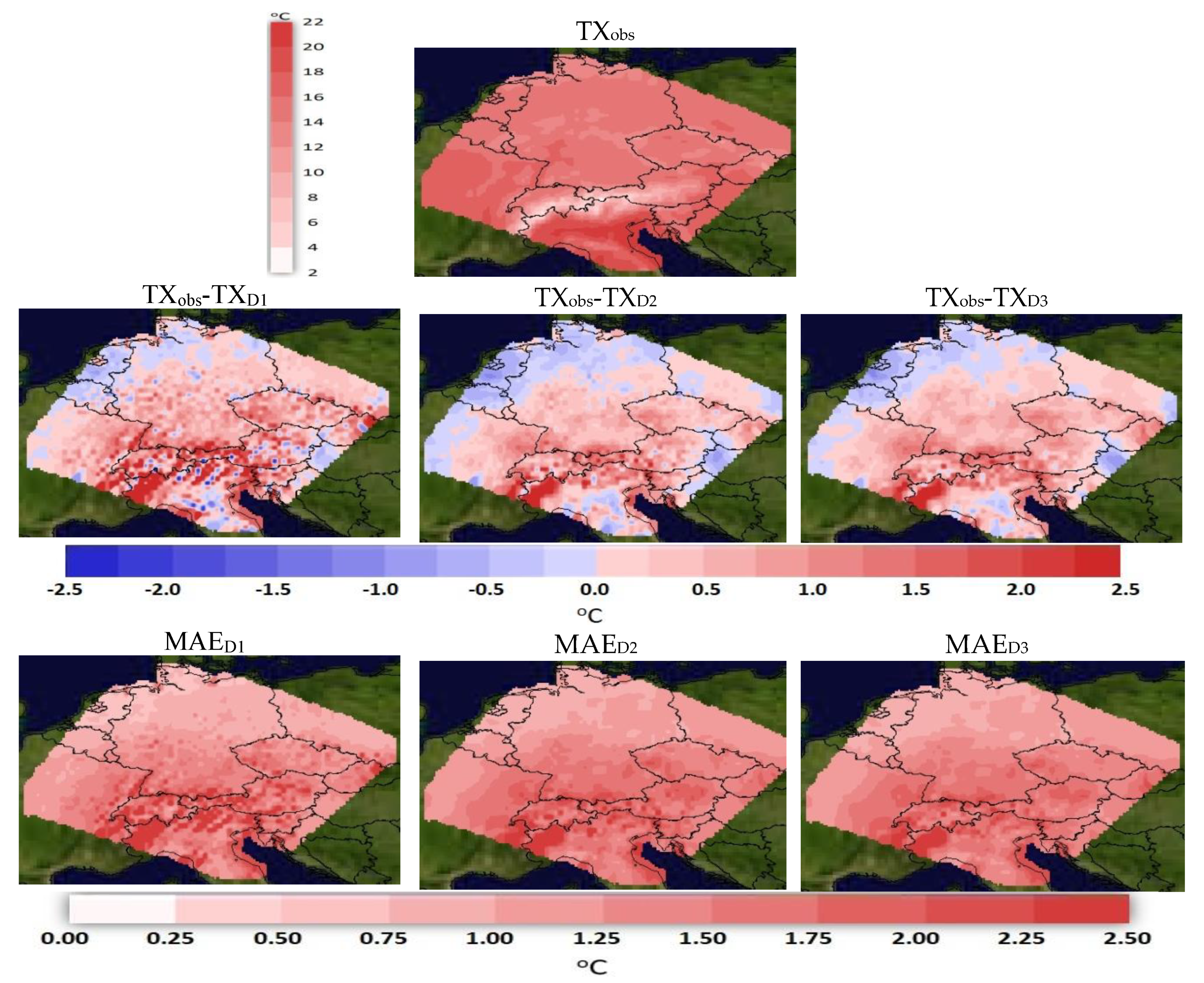
3.2. Maximum Temperature

The model underestimates annual maximum temperature in a major part of the domain. The highest differences are found in the Alps region (Figure 4). This trend, as well as the spatial pattern, do not change with the increase of the spatial resolution. However, model performance is better when increasing the spatial resolution from 36 (D1) to 12 km (D2), while a minor change is found when the spatial resolution is further increased (i.e., 4 km (D3)). This is also supported by the domain wide average values of the statistical metrics (

Table 4. Annual maximum temperature statistical analysis (°C).

	D1 (36 km)	D2 (12 km)	D3 (4 km)	Δij (D2-D1)	Δij (D3-D2)
Mean Observed	14.91			-	-
Mean Predicted	14.33	14.41	14.44	-	-
Positive BIAS	0.40	0.24	0.23	0.49	0.14
Negative BIAS	−0.87	−0.68	−0.64	−0.50	−0.11
RMSE	1.14	0.81	0.76	0.82	0.22
IoA	0.95	0.98	0.99	0.98	1.00
MAE	0.76	0.59	0.56	0.49	0.13

).

The seasonal maximum temperature plots present a similar spatial pattern between the three domains for each season (Figures S5–S8 of Supplementary Material). During autumn, the model overestimates maximum temperature over the domain with the exception of the Alps region (Figure S5). Increasing the spatial resolution from 36 (D1) to 4 km (D3) improves the statistical measures (Table S5) suggesting that the finer domain better represents autumn maximum temperature. However, the improvement between 36 (D1) and 12 km (D2) is more important compared to the improvement between 12 (D2) and 4 km (D3). During winter, the model underestimates maximum temperature in major part of the domain (Figure S6). Underestimation is mainly noted over Italy, the Eastern Alps and most part of Switzerland. Increasing the spatial resolution from 36 (D1) to 12 km (D2) improves the statistical measures (Table S6) but no significant change is found when the spatial resolution is further increased (i.e., 4 km (D3)). During spring and summer, the model underestimates maximum temperature in most parts of the domain (Figures S7 and S8). Increasing the spatial resolution from 36 (D1) to 12 km (D2) improves statistical measures (Tables S3 and S4) but no significant change is found when the spatial resolution is further increased (i.e., 4 km (D3)).

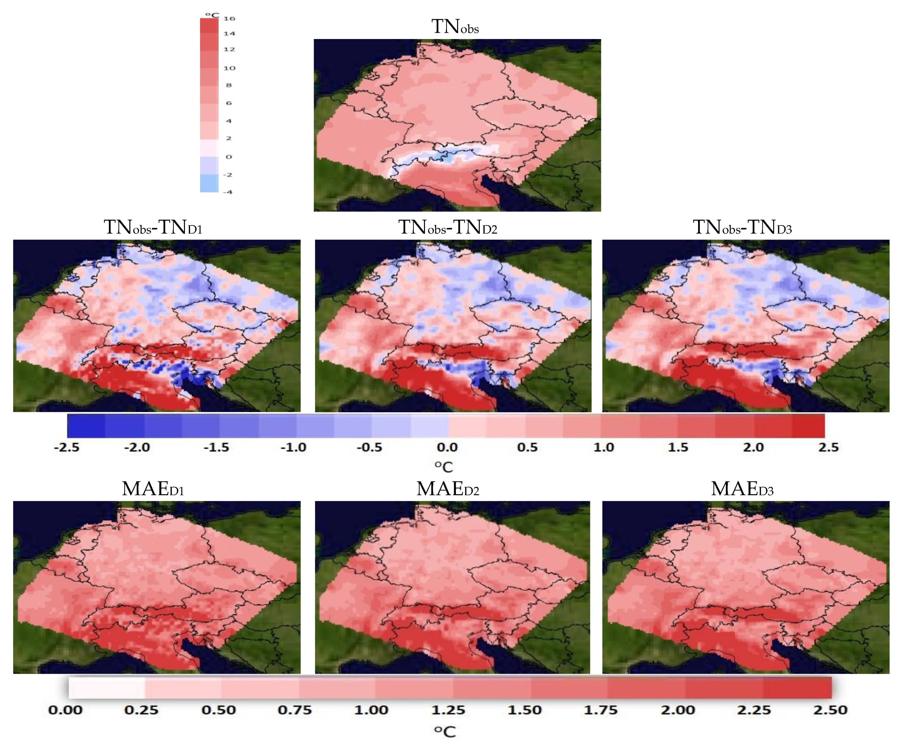
3.3. Minimum Temperature

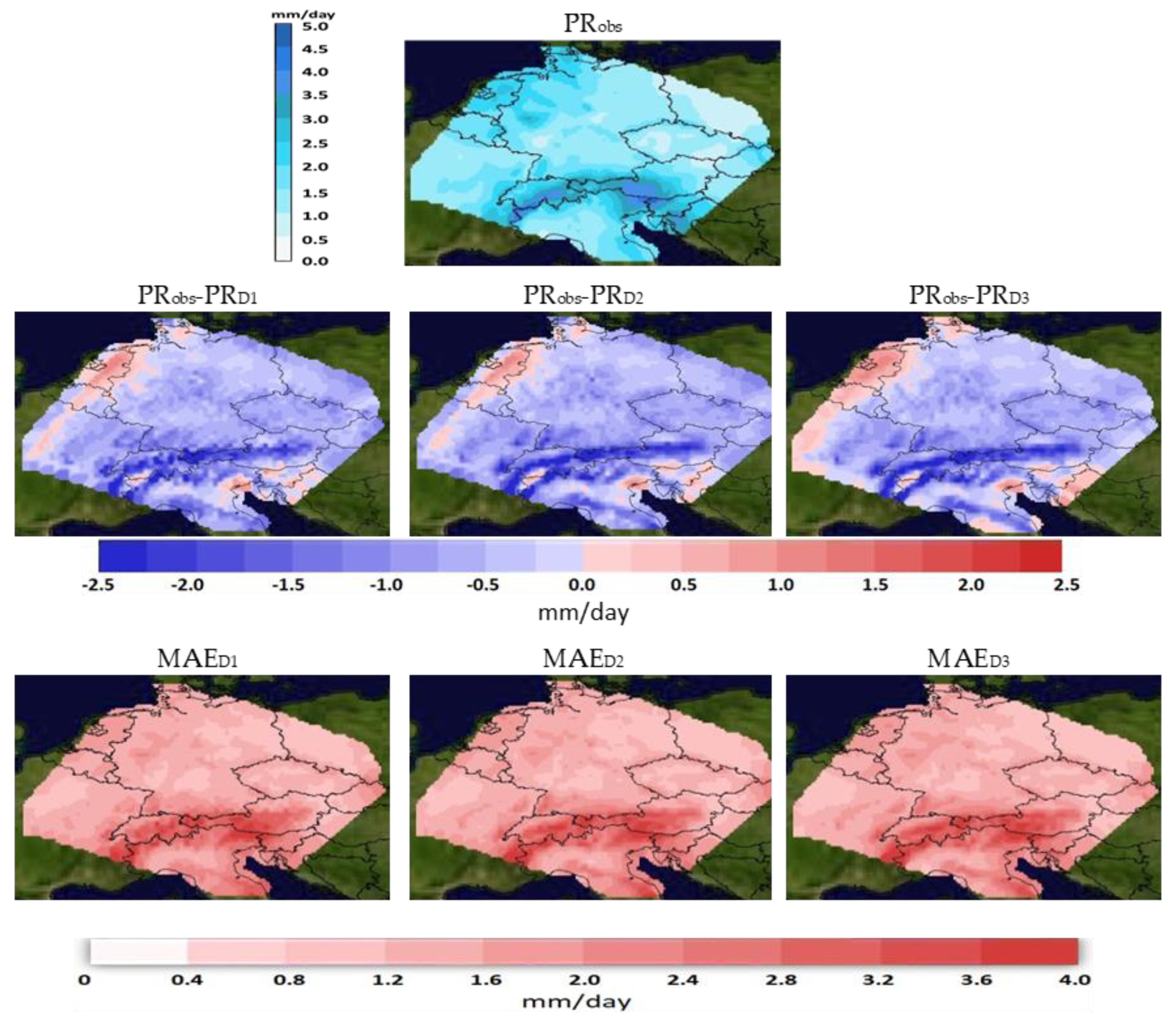
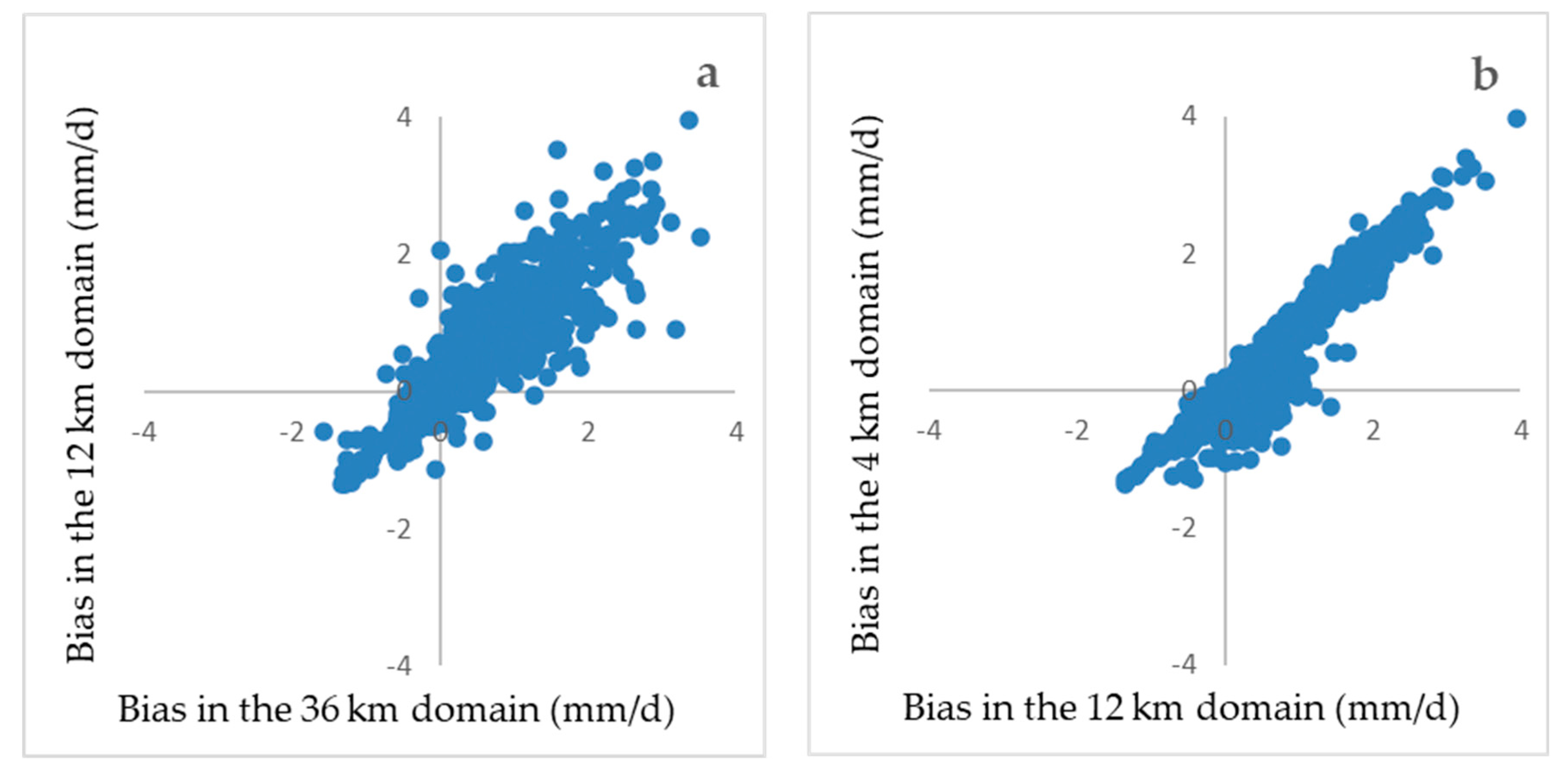
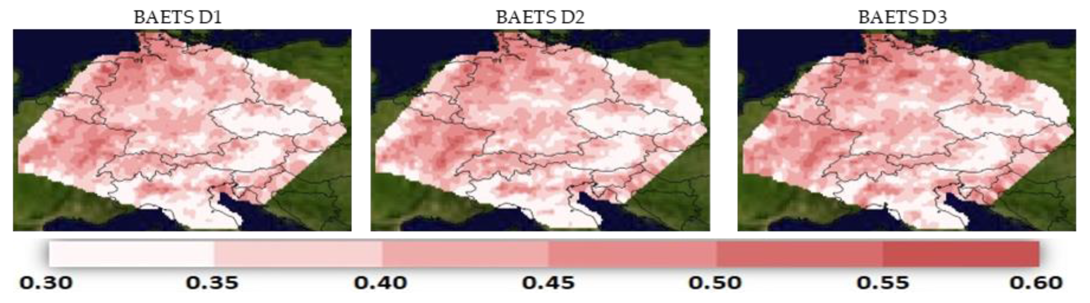
The model underestimates annual minimum temperature in major part of the domain for all three grid resolutions used. The highest differences are found over northern Italy and the Alps region (Figure 5). This trend, as well as the spatial pattern, do not change with the increase of the spatial resolution. Model performance does not change in the higher spatial resolution grids (i.e., 12 (D2) and 4 km (D3)) compared to the 36 km (D1) domain, except for the positive bias that is improved on the finer nested domain (

Table 5. Annual minimum temperature statistical analysis (°C).

	D1 (36 km)	D2 (12 km)	D3 (4 km)	Δij (D2-D1)	Δij (D3-D2)
Mean Observed	5.73			-	-
Mean Predicted	5.23	5.11	5.00	-	-
Positive BIAS	0.55	0.44	0.39	0.40	0.12
Negative BIAS	−1.00	−1.00	−1.07	−0.35	−0.14
RMSE	1.27	1.27	1.31	0.63	0.21
IoA	0.92	0.92	0.92	0.98	1.00
MAE	0.85	0.85	0.91	0.35	0.14

).

The seasonal minimum temperature plots present a similar spatial pattern between the three domains for each season (Figures S9–S12 of Supplementary Material). For all seasons, mean predicted values are lower than the observed ones, with domain D1 presenting a better closure with observations compared to D2 and D3, mainly as a result of the gradual increase in the negative bias when moving from D1 to D2 and D3. This finding might be related to the stronger negative bias in precipitation (Tables S13–S16) when moving to finer grid resolutions that leads to gradually larger evaporative cooling. During autumn the model overestimates min temperature over the eastern border of the domain and north-east Italy (Figure S9). Increasing the spatial resolution does not improve the statistical measures except for the positive bias (Table S9). During winter the model underestimates min temperature mainly over north-west Italy and the Alps region while there is a mixed trend for the rest of the domain (Figure S10). Increasing the spatial resolution from 36 (D1) to 4 km (D3) causes a slight improvement on the positive bias but the rest of the statistical measures do not improve (Table S10). During spring and summer, the model underestimates min temperature in most part of the domain (Figures S11 and S12). Increasing the spatial resolution from 36 (D1) to 4 km (D3) does not improve the statistical measures except for the positive bias (Table S1).

3.4. Precipitation

The model overestimates annual precipitation in major part of the domain except the regions at the west and south east borders (Figure 6). Simulated and observed data are in quite good agreement in areas with precipitation rates below 3mm/day with the model being able to represent the precipitation range within a ±25% accuracy. However, for high-precipitation areas such as the alpine and mountainous regions, differences are quite high (up to 2.5 mm/day overestimation by the model) that are probably related to known E-OBS deficiencies in properly capturing the correct range of precipitation in regions with sparse and uneven station coverage. This trend as well as the spatial pattern do not change with the increase of the spatial resolution.

The statistical analysis suggests that model performance is slightly better when increasing the spatial resolution from 36 (D1) to 12 km (D2) while further increasing spatial resolution to 4 km (D1) has a negligible effect (

Table 6. Annual mean precipitation statistical analysis (mm/day).

	D1 (36 km)	D2 (12 km)	D3 (4 km)	Δij (D2-D1)	Δij (D3-D2)
Mean Observed	1.97			-	-
Mean Predicted	2.49	2.48	2.42	-	-
Positive MB	0.67	0.66	0.65	0.00	0.66
Negative MB	−0.38	−0.35	−0.33	4.97	−2.51
RMSE	0.81	0.80	0.79	2.44	−0.48
IoA	0.77	0.78	0.79	−0.74	0.12
MAE	0.62	0.62	0.60	0.96	−1.39

). Minor improvements in models’ performances on a daily, seasonal or annual basis when increasing the grid spacing to convection permitting simulations have also been found by other studies as well (e.g., [18,24,44,45]) suggesting that sub-daily timeframes need to be considered in such cases for improvements to be seen.

Investigating the grid size effect, we compare the biases, i.e., simulated minus observed daily values, for domains D1 against D2 (Figure 7a) and D2 against D3 (Figure 7b). The biases between the D2 and D3 simulations are very similar (mostly fall on the diagonal) with slightly lower precipitation rates for D3 domain (below the diagonal) and smaller in range than the D1 simulation (Figure 7a). As a result, the projection improvement is higher for D2 compared to D1, with no significant added value being seen for D3 compared to D2. In addition, the spatial error variability derived for the three domain resolutions shows only a minor improvement in the spatial error variability (0.58 mm/d for D1, 0.56 mm/d for D2 and 0.55 mm/d for D3) with the reduction of the grid resolution.

The seasonal precipitation plots present a similar spatial trend between the three domains for each season (Figures S13–S16 of Supplementary Material). During autumn, the model underestimates precipitation mainly at the north-west and south-east part of the domain (Figure S13) in all resolutions considered, while the statistical analysis suggests negligible effect of the grid size on the results (Table S13). During winter the model underestimates precipitation mainly at the north-west part of the domain (Figure S14). The statistical analysis suggests that model performance is negligibly affected when increasing the spatial resolution from 36 (D1) to 12 km (D2), while further increasing to 4 km (D3) spatial resolution does not improve statistics (Table S14). During spring, the model overestimates precipitation at major part of the domain (Figure S15). The statistical analysis suggests that increasing the spatial resolution from 36 (D1) to 12 km (D2) as well as from 12 (D2) to 4 km (D3) does not modify significantly model performance. During summer, the model overestimates precipitation at major parts of the domain with the largest values over the high elevated regions of northern Italy (Figure S16). This positive bias is caused by the cumulus parameterization of the model that overestimates convective precipitation. The statistical analysis suggests that model performance is worsened when increasing the spatial resolution from 36 (D1) to 12 km (D2) while further increasing to 4 km (D1) spatial resolution slightly improves statistics compared to 12 km (D2) (Table S16).

Increasing the spatial resolution from 36 (D1) to 4 km (D3) suggests that annual mean BAETS, which measures the fraction of observed and/or forecast events that were correctly predicted, is slightly affected on average over the domain (

Table 7. Annual mean BAETS.

	D1 (36 km)	D2 (12 km)	D3 (4 km)
BAETS	0.421	0.417	0.423

), presenting a mixed trend spatially with small changes, apart from a few cells across the domain (Figure 8 and Figure 9). The number of these cells is higher when increasing the spatial resolution from 36 (D1) to 12 km (D2), where a negative impact is dominant among these cells, compared to the impact when increasing the spatial resolution from 12 (D2) to 4 km (D3). The same trend with annual BAETS analysis is also found in the seasonal BAETS analysis (Figures S17 and S18, Table S17). However, during summer, the model presents significantly lower BAETS skill score compared to the rest of the seasons.

4. Conclusions

WRF performance over central Europe for mean and maximum temperature, both annually and seasonally, is better when increasing the spatial resolution from 36 to 12 km, while a minor change is found when the grid resolution is further increased to 4 km as shown by the statistical analysis performed in this study. The exception is the maximum temperature during autumn, which is further improved when the spatial resolution is increased to 4 km. However, the improvement between 36 and 12 km is much more important compared to the improvement between 12 and 4 km. Model performance for both annual and seasonal minimum temperatures does not change in the finer spatial resolution grids (i.e., 12 and 4 km) compared to the 36 km domain, except for the negative bias, which is improved on both nested domains. Model performance for annual and seasonal mean precipitation as well for annual and seasonal mean BAETS, which measures the fraction of observed and/or forecast events that were correctly predicted, is slightly affected when increasing the spatial resolution from 36 to 4 km. The model’s statistical performance for precipitation is quite good in areas with low precipitation rates, while in high-precipitation areas such as the mountainous regions, it is not. Precipitation predictability is slightly worsened when increasing the spatial resolution from 36 to 12 km, while further increasing it to 4 km has a negligible or minor effect. BAETS presents a weak correlation with the spatial resolution, presenting similar behavior over the three domains; during summer, the model presents significantly lower BAETS skill score compared to the rest of the seasons.

WRF captures the basic features of temperature and precipitation in magnitude, space and time over central Europe for all three grid size resolutions used in the present study. The results highlight some seasonal deficiencies and suggest their improved representation when analysis is carried out in the 12 km domain compared to the 36 km one. The model’s skill is not better when further decreasing grid spacing (i.e., when comparing the results of the 4 km against the 12 km domain). This implies that downscaling produces skillful information up to 12 km grid size that is used in this study, however, the finer grid resolution of 4 km used does not provide statistically significant improved representation of annual or seasonal temperature and precipitation. This finding does not necessarily mean that model performance is not improved when the finer resolution of 4 km used in this study is employed. As a matter of fact, the better representation of vegetation variability, complex topography and coastlines of the fine resolution, which are significant components of the physical system, are anticipated to improve the model’s performance. The statistically small improvement found here for the finer domain could be related to the comparison with the E-OBS coarser resolution than the 4 km used here. We acknowledge that an evaluation based on the high-resolution data would potentially preserve the finer resolution details and the decreased improvement in the statistical analysis seen for the finer resolution compared to the 12 km domain could be a result of the averaging. On the other hand, if processes are better captured at higher resolution, improvements are expected to be visible even when regridded to coarser resolution. Still, this points out the crucial need for high resolution and quality observations over the European domain for improved representation of such parameters in very fine scales.

References

1. Giorgi, F.; Gutowski, W.J. Coordinated Experiments for Projections of Regional Climate Change. Curr. Clim. Chang. Rep. 2016, 2, 202–210. [Google Scholar] [CrossRef] [Green Version]
2. Knutti, R.; Sedláček, J. Robustness and Uncertainties in the New CMIP5 Climate Model Projections. Nat. Clim. Chang. 2013, 3, 369–373. [Google Scholar] [CrossRef]
3. Giorgi, F.; Gutowski, W.J. Regional Dynamical Downscaling and the CORDEX Initiative. Annu. Rev. Environ. Resour. 2015, 40, 467–490. [Google Scholar] [CrossRef]
4. Jacob, D.; Teichmann, C.; Sobolowski, S.; Katragkou, E.; Anders, I.; Belda, M.; Benestad, R.; Boberg, F.; Buonomo, E.; Cardoso, R.M.; et al. Regional Climate Downscaling over Europe: Perspectives from the EURO-CORDEX Community. Reg. Environ. Chang. 2020, 20, 51. [Google Scholar] [CrossRef]
5. Giorgi, F.; Mearns, L.O. Approaches to the Simulation of Regional Climate Change: A Review. Rev. Geophys. 1991, 29, 191–216. [Google Scholar] [CrossRef]
6. Flocas, H.A.; Hatzaki, M.; Tolika, K.; Anagnostopoulou, C.; Kostopoulou, E.; Giannakopoulos, C.; Kolokytha, E.; Tegoulias, I. Ability of RCM/GCM Couples to Represent the Relationship of Large Scale Circulation to Climate Extremes over the Mediterranean Region. Clim. Res. 2011, 46, 197–209. [Google Scholar] [CrossRef] [Green Version]
7. Rummukainen, M. State-of-the-Art with Regional Climate Models. WIREs Clim. Chang. 2010, 1, 82–96. [Google Scholar] [CrossRef]
8. Poan, E.D.; Gachon, P.; Laprise, R.; Aider, R.; Dueymes, G. Investigating Added Value of Regional Climate Modeling in North American Winter Storm Track Simulations. Clim. Dyn. 2018, 50, 1799–1818. [Google Scholar] [CrossRef] [Green Version]
9. Vautard, R.; Gobiet, A.; Jacob, D.; Belda, M.; Colette, A.; Déqué, M.; Fernández, J.; García-Díez, M.; Goergen, K.; Güttler, I.; et al. The Simulation of European Heat Waves from an Ensemble of Regional Climate Models within the EURO-CORDEX Project. Clim. Dyn. 2013, 41, 2555–2575. [Google Scholar] [CrossRef]
10. Kotlarski, S.; Keuler, K.; Christensen, O.B.; Colette, A.; Déqué, M.; Gobiet, A.; Goergen, K.; Jacob, D.; Lüthi, D.; Van Meijgaard, E.; et al. Regional Climate Modeling on European Scales: A Joint Standard Evaluation of the EURO-CORDEX RCM Ensemble. Geosci. Model Dev. 2014, 7, 1297–1333. [Google Scholar] [CrossRef] [Green Version]
11. Jaeger, E.B.; Anders, I.; Lüthi, D.; Rockel, B.; Schär, C.; Seneviratne, S.I. Analysis of ERA 40-Driven CLM Simulations for Europe. Meteorol. Z. 2008, 17, 349–367. [Google Scholar] [CrossRef]
12. van Roosmalen, L.; Christensen, J.H.; Butts, M.B.; Jensen, K.H.; Refsgaard, J.C. An Intercomparison of Regional Climate Model Data for Hydrological Impact Studies in Denmark. J. Hydrol. 2010, 380, 406–419. [Google Scholar] [CrossRef]
13. Heikkilä, U.; Sandvik, A.; Sorteberg, A. Dynamical Downscaling of ERA-40 in Complex Terrain Using the WRF Regional Climate Model. Clim. Dyn. 2011, 37, 1551–1564. [Google Scholar] [CrossRef] [Green Version]
14. Giorgi, F.; Marinucci, M.R. An Investigation of the Sensitivity of Simulated Precipitation to Model Resolution and Its Implications for Climate Studies. Mon. Weather Rev. 1996, 124, 148–166. [Google Scholar] [CrossRef] [Green Version]
15. Leung, L.R.; Qian, Y. The Sensitivity of Precipitation and Snowpack Simulations to Model Resolution via Nesting in Regions of Complex Terrain. J. Hydrometeorol. 2003, 4, 1025–1043. [Google Scholar] [CrossRef]
16. Li, Y.; Lu, G.; Wu, Z.; He, H.; Shi, J.; Ma, Y.; Weng, S. Evaluation of Optimized WRF Precipitation Forecast over a Complex Topography Region during Flood Season. Atmosphere 2016, 7, 145. [Google Scholar] [CrossRef] [Green Version]
17. Rauscher, S.A.; Coppola, E.; Piani, C.; Giorgi, F. Resolution Effects on Regional Climate Model Simulations of Seasonal Precipitation over Europe. Clim. Dyn. 2010, 35, 685–711. [Google Scholar] [CrossRef]
18. Chan, S.C.; Kendon, E.J.; Fowler, H.J.; Blenkinsop, S.; Ferro, C.A.T.; Stephenson, D.B. Does Increasing the Spatial Resolution of a Regional Climate Model Improve the Simulated Daily Precipitation? Clim. Dyn. 2013, 41, 1475–1495. [Google Scholar] [CrossRef]
19. Prein, A.F.; Gobiet, A.; Truhetz, H.; Keuler, K.; Goergen, K.; Teichmann, C.; Fox Maule, C.; van Meijgaard, E.; Déqué, M.; Nikulin, G.; et al. Precipitation in the EURO-CORDEX 0.11° and 0.44° simulations: High resolution, high benefits? Clim. Dyn. 2016, 46, 383–412. [Google Scholar] [CrossRef] [Green Version]
20. Torma, C.; Giorgi, F.; Coppola, E. Added Value of Regional Climate Modeling over Areas Characterized by Complex Terrain-Precipitation over the Alps. J. Geophys. Res. 2015, 120, 3957–3972. [Google Scholar] [CrossRef]
21. Powers, J.G.; Klemp, J.B.; Skamarock, W.C.; Davis, C.A.; Dudhia, J.; Gill, D.O.; Coen, J.L.; Gochis, D.J.; Ahmadov, R.; Peckham, S.E.; et al. The Weather Research and Forecasting Model: Overview, System Efforts, and Future Directions. Bull. Am. Meteorol. Soc. 2017, 98, 1717–1737. [Google Scholar] [CrossRef]
22. Skamarock, C.; Klemp, B.; Dudhia, J.; Gill, O.; Barker, D.; Duda, G.; Huang, X.; Wang, W.; Powers, G. A Description of the Advanced Research WRF Version 3; University Corporation for Atmospheric Research: Boulder, CO, USA, 2008. [Google Scholar] [CrossRef]
23. Haylock, M.R.; Hofstra, N.; Klein Tank, A.M.G.; Klok, E.J.; Jones, P.D.; New, M. A European Daily High-Resolution Gridded Data Set of Surface Temperature and Precipitation for 1950-2006. J. Geophys. Res. Atmos. 2008, 113. [Google Scholar] [CrossRef] [Green Version]
24. Prein, A.F.; Gobiet, A.; Suklitsch, M.; Truhetz, H.; Awan, N.K.; Keuler, K.; Georgievski, G. Added Value of Convection Permitting Seasonal Simulations. Clim. Dyn. 2013, 41, 2655–2677. [Google Scholar] [CrossRef] [Green Version]
25. Katragkou, E.; Garciá-Diéz, M.; Vautard, R.; Sobolowski, S.; Zanis, P.; Alexandri, G.; Cardoso, R.M.; Colette, A.; Fernandez, J.; Gobiet, A.; et al. Regional Climate Hindcast Simulations within EURO-CORDEX: Evaluation of a WRF Multi-Physics Ensemble. Geosci. Model Dev. 2015, 8, 603–618. [Google Scholar] [CrossRef] [Green Version]
26. Pavlidis, V.; Katragkou, E.; Prein, A.; Georgoulias, A.K.; Kartsios, S.; Zanis, P.; Karacostas, T. Investigating the Sensitivity to Resolving Aerosol Interactions in Downscaling Regional Model Experiments with WRFv3.8.1 over Europe. Geosci. Model Dev. 2020, 13, 2511–2532. [Google Scholar] [CrossRef]
27. Knist, S.; Goergen, K.; Simmer, C. Evaluation and Projected Changes of Precipitation Statistics in Convection-Permitting WRF Climate Simulations over Central Europe. Clim. Dyn. 2020, 55, 325–341. [Google Scholar] [CrossRef] [Green Version]
28. Jerez, S.; López-Romero, J.M.; Turco, M.; Lorente-Plazas, R.; Gómez-Navarro, J.J.; Jiménez-Guerrero, P.; Montávez, J.P. On the Spin-Up Period in WRF Simulations Over Europe: Trade-Offs Between Length and Seasonality. J. Adv. Model. Earth Syst. 2020, 12. [Google Scholar] [CrossRef] [Green Version]
29. Cornes, R.C.; van der Schrier, G.; van den Besselaar, E.J.M.; Jones, P.D. An Ensemble Version of the E-OBS Temperature and Precipitation Data Sets. J. Geophys. Res. Atmos. 2018, 123, 9391–9409. [Google Scholar] [CrossRef] [Green Version]
30. Cardell, M.F.; Romero, R.; Amengual, A.; Homar, V.; Ramis, C. A Quantile–Quantile Adjustment of the EURO-CORDEX Projections for Temperatures and Precipitation. Int. J. Climatol. 2019, 39, 2901–2918. [Google Scholar] [CrossRef]
31. Kotlarski, S.; Szabó, P.; Herrera, S.; Räty, O.; Keuler, K.; Soares, P.M.; Cardoso, R.M.; Bosshard, T.; Pagé, C.; Boberg, F.; et al. Observational Uncertainty and Regional Climate Model Evaluation: A Pan-European Perspective. Int. J. Climatol. 2019, 39, 3730–3749. [Google Scholar] [CrossRef] [Green Version]
32. Lenderink, G. Exploring Metrics of Extreme Daily Precipitation in a Large Ensemble of Regional Climate Model Simulations. Clim. Res. 2010, 44, 151–166. [Google Scholar] [CrossRef]
33. Min, E.; Hazeleger, W.; Van Oldenborgh, G.J.; Sterl, A. Evaluation of Trends in High Temperature Extremes in North-Western Europe in Regional Climate Models. Environ. Res. Lett. 2013, 8. [Google Scholar] [CrossRef] [Green Version]
34. Nikulin, G.; Kjellström, E.; Hansson, U.; Strandberg, G.; Ullerstig, A. Evaluation and Future Projections of Temperature, Precipitation and Wind Extremes over Europe in an Ensemble of Regional Climate Simulations. Tellus Ser. Dyn. Meteorol. Oceanogr. 2011, 63, 41–55. [Google Scholar] [CrossRef] [Green Version]
35. Velikou, K.; Tolika, K.; Anagnostopoulou, C.; Zanis, P. Sensitivity Analysis of RegCM4 Model: Present Time Simulations over the Mediterranean. Theor. Appl. Climatol. 2019, 136, 1185–1208. [Google Scholar] [CrossRef]
36. Fantini, A.; Raffaele, F.; Torma, C.; Bacer, S.; Coppola, E.; Giorgi, F.; Ahrens, B.; Dubois, C.; Sanchez, E.; Verdecchia, M. Assessment of Multiple Daily Precipitation Statistics in ERA-Interim Driven Med-CORDEX and EURO-CORDEX Experiments against High Resolution Observations. Clim. Dyn. 2018, 51, 877–900. [Google Scholar] [CrossRef]
37. Bellprat, O.; Kotlarski, S.; Thi, D.L.; Schär, C. Exploring Perturbed Physics Ensembles in a Regional Climate Model. J. Clim. 2012, 25, 4582–4599. [Google Scholar] [CrossRef]
38. Hofstra, N.; Haylock, M.; New, M.; Jones, P.D. Testing E-OBS European High-Resolution Gridded Data Set of Daily Precipitation and Surface Temperature. J. Geophys. Res. Atmospheres 2009, 114. [Google Scholar] [CrossRef]
39. Hofstra, N.; New, M.; McSweeney, C. The Influence of Interpolation and Station Network Density on the Distributions and Trends of Climate Variables in Gridded Daily Data. Clim. Dyn. 2010, 35, 841–858. [Google Scholar] [CrossRef]
40. Maraun, D.; Osborn, T.J.; Rust, H.W. The Influence of Synoptic Airflow on UK Daily Precipitation Extremes. Part II: Regional Climate Model and E-OBS Data Validation. Clim. Dyn. 2012, 39, 287–301. [Google Scholar] [CrossRef]
41. Boris, S. Correction of Precipitation Measurements: ETH/IAHS/WMO Workshop on the Correction of Precipitation Measurements, Zurich, 1–3 April 1985; ETH/IAHS/WMO Workshop on the Correction of Precipitation Measurements, Ed.; Geographisches Institut, Eidgenössische Technische Hochschule: Zürich, Switzerland, 1986. [Google Scholar]
42. Prein, A.F.; Gobiet, A. Impacts of Uncertainties in European Gridded Precipitation Observations on Regional Climate Analysis. Int. J. Climatol. 2017, 37, 305–327. [Google Scholar] [CrossRef]
43. Mesinger, F. Bias Adjusted Precipitation Threat Scores. Adv. Geosci. 2008, 16, 137–142. [Google Scholar] [CrossRef] [Green Version]
44. Ban, N.; Schmidli, J.; Schär, C. Evaluation of the Convection-Resolving Regional Climate Modeling Approach in Decade-Long Simulations. J. Geophys. Res. 2014, 119, 7889–7907. [Google Scholar] [CrossRef]
45. Fosser, G.; Khodayar, S.; Berg, P. Benefit of Convection Permitting Climate Model Simulations in the Representation of Convective Precipitation. Clim. Dyn. 2014, 44, 45–60. [Google Scholar] [CrossRef] [Green Version]
Figure 1. Weather Research and Forecasting (WRF) multi-nesting domain configuration approach with increasing domain resolution of 36, 12 and 4 km.
Atmosphere 12 00278 g001
Figure 2. Spatial distribution plots for annual mean temperature: observed data (upper panel), differences between observed and simulated data for the three nested domains (middle row), and the related mean absolute error (MAE) (lower row).
Atmosphere 12 00278 g002
Figure 3. Scatter plots presenting (a) D1 (x-axis) against D2 (y-axis) and (b) D2 (x-axis) against D3 (y-axis) simulated annual temperature biases for all grids considered.
Atmosphere 12 00278 g003
Figure 4. Spatial distribution plots for annual max temperature: observed data (upper panel), differences between observed and simulated data for the three nested domains (middle row), and the related MAE (lower row).
Atmosphere 12 00278 g004
Figure 5. Spatial distribution plots for annual minimum temperature: observed data (upper panel), differences between observed and simulated data for the three nested domains (middle row), and the related MAE (lower row).
Atmosphere 12 00278 g005
Figure 6. Spatial distribution plots for annual mean precipitation: observed data (upper panel), differences between observed and simulated data for the three nested domains (middle row), and the related MAE (lower row).
Atmosphere 12 00278 g006
Figure 7. Scatter plots presenting (a) D1 (x-axis) against D2 (y-axis) and (b) D2 (x-axis) against D3 (y-axis) simulated annual precipitation biases for all grid cells considered.
Atmosphere 12 00278 g007
Figure 8. Annual mean BAETS spatial distribution plots.
Atmosphere 12 00278 g008
Figure 9. Annual mean BAETS change spatial distribution plots.
Atmosphere 12 00278 g009