
Interannual Variability of the GNSS Precipitable Water Vapor in the Global Tropics

 , and
, and
Abstract
:1. Introduction
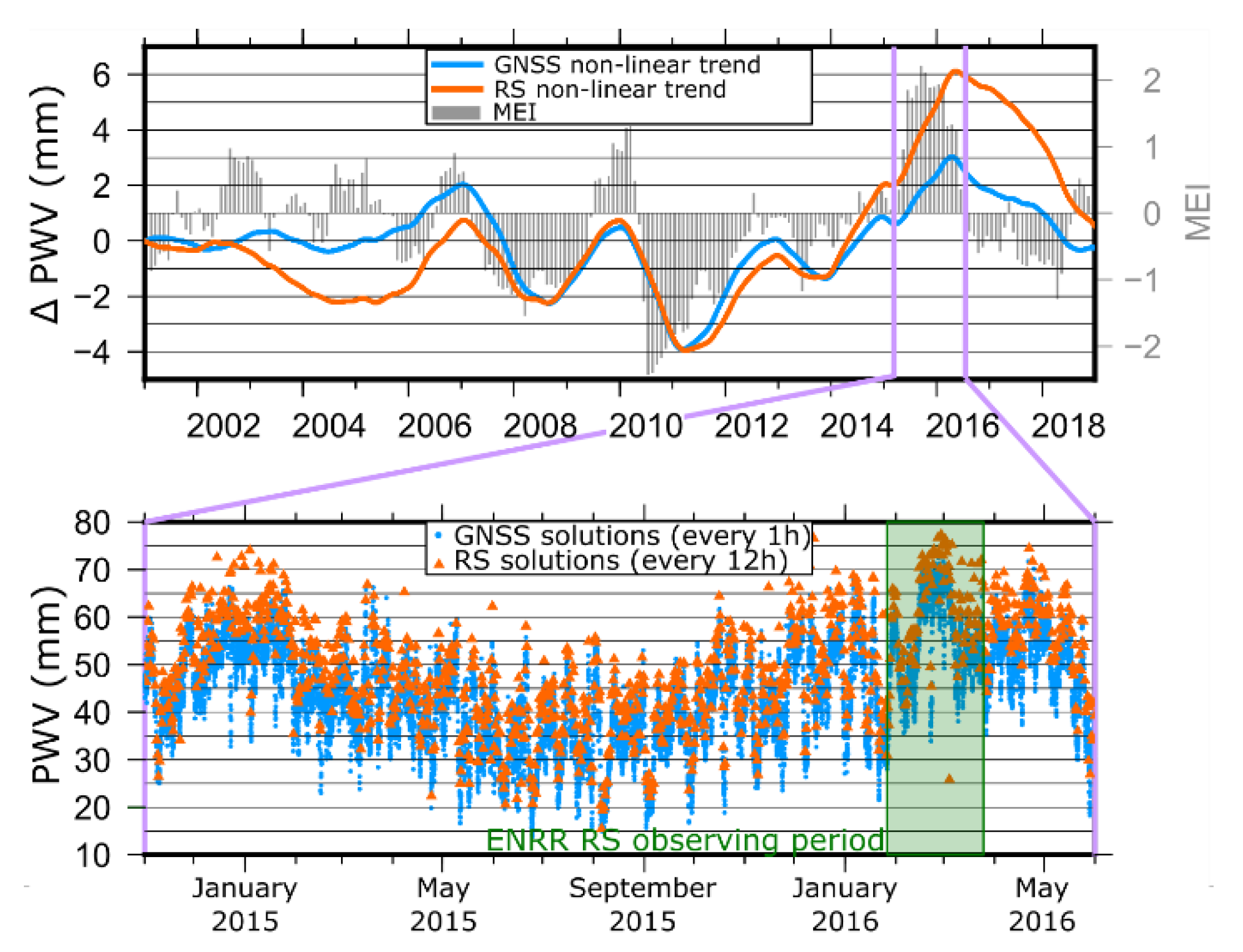
2. Materials and Methods
3. Results
3.1. Non-Linear Long-Term Variability
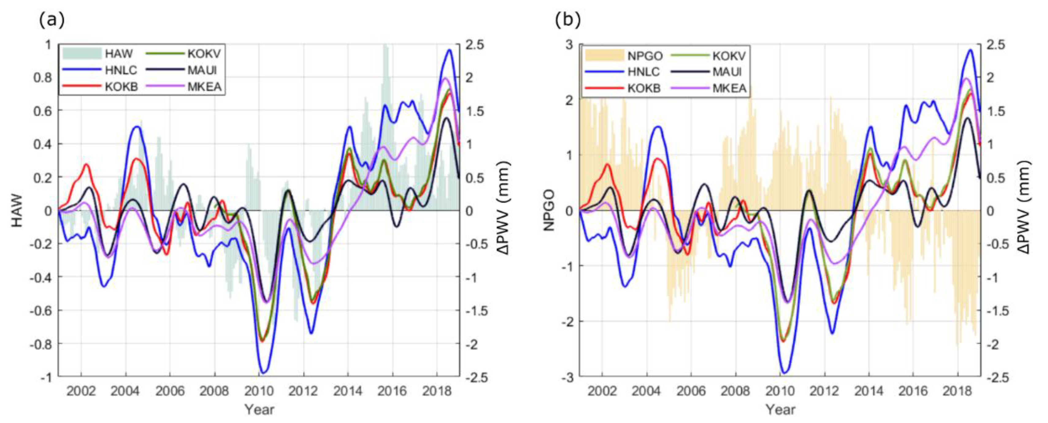
3.1.1. Pacific Related Climate Indices
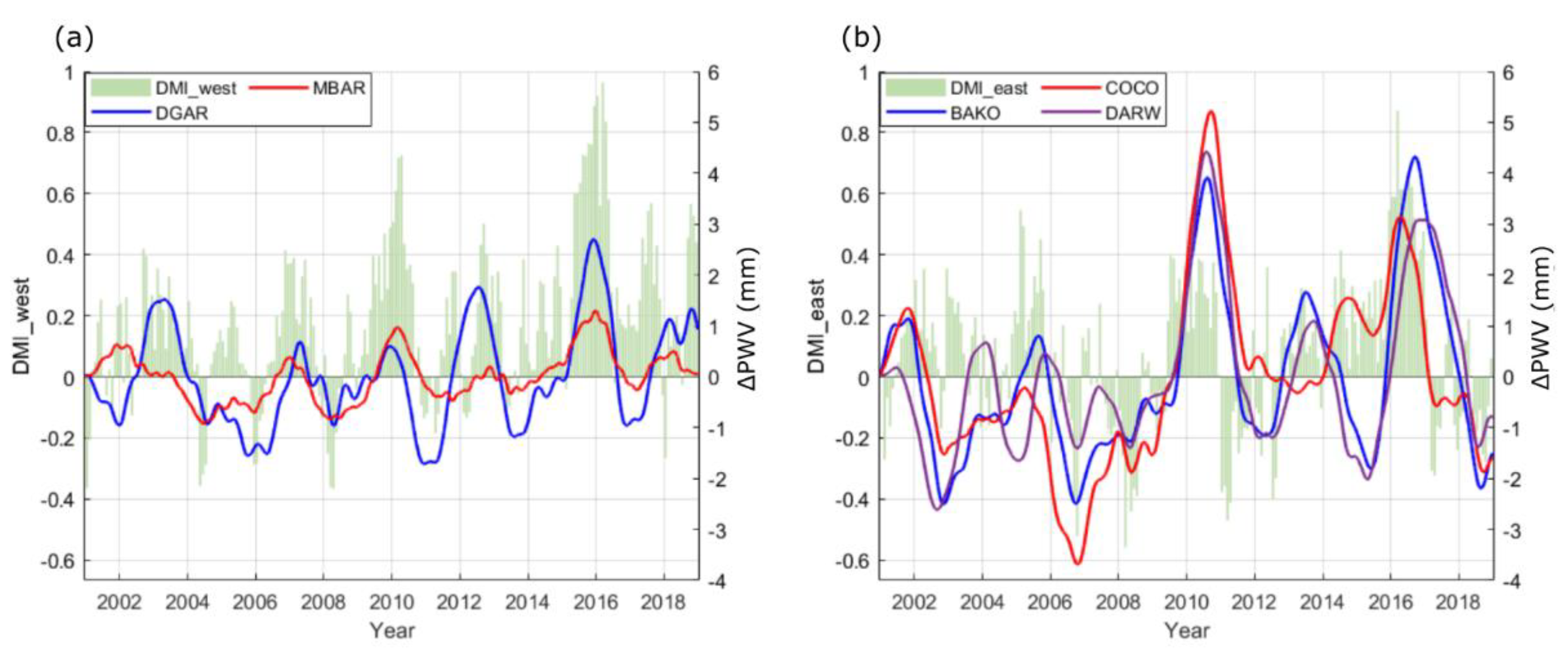
3.1.2. Indian Ocean Related Climate Indices
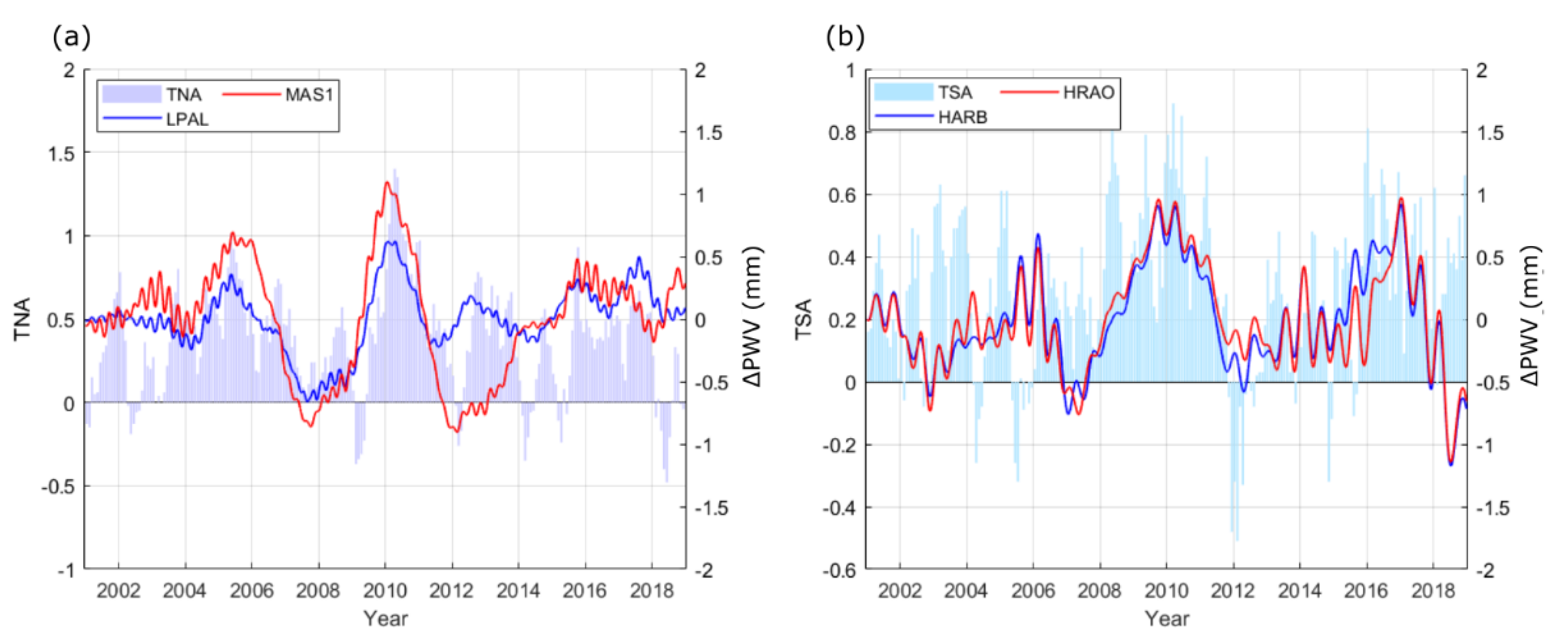
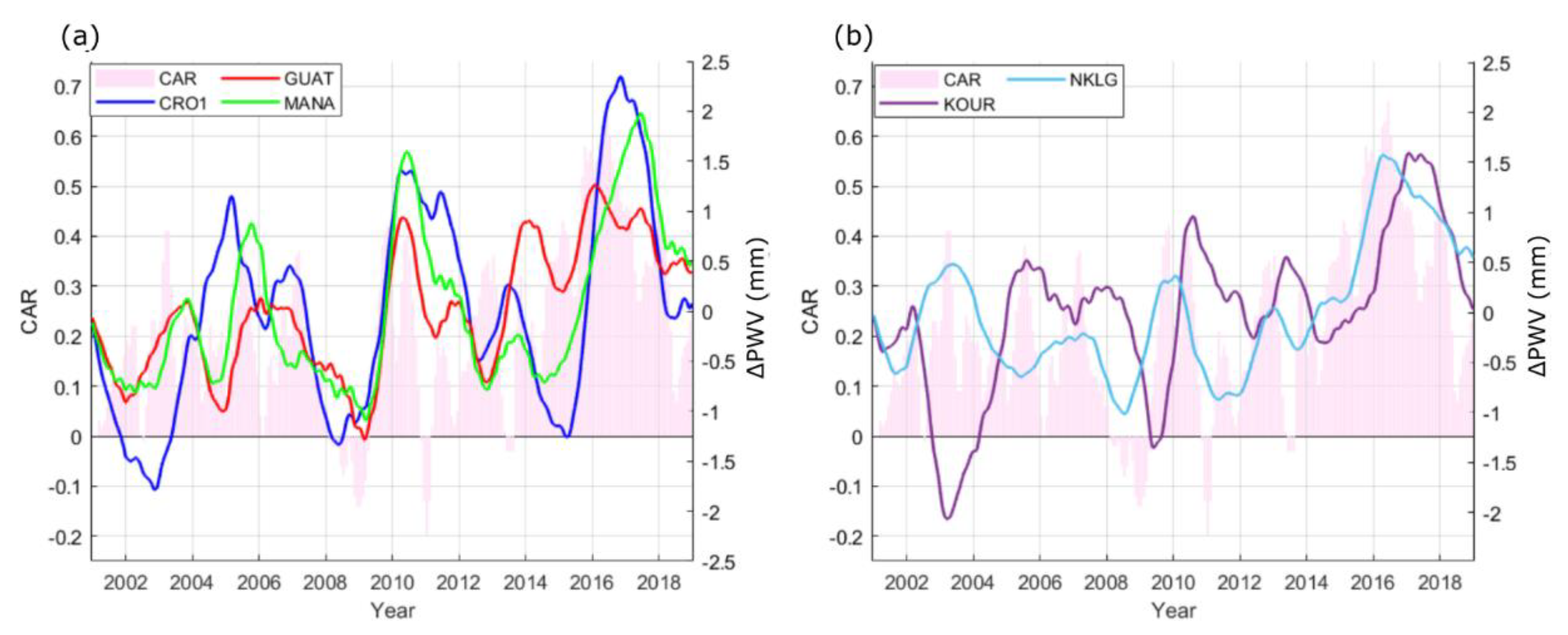
3.1.3. Atlantic Related Climate Indices
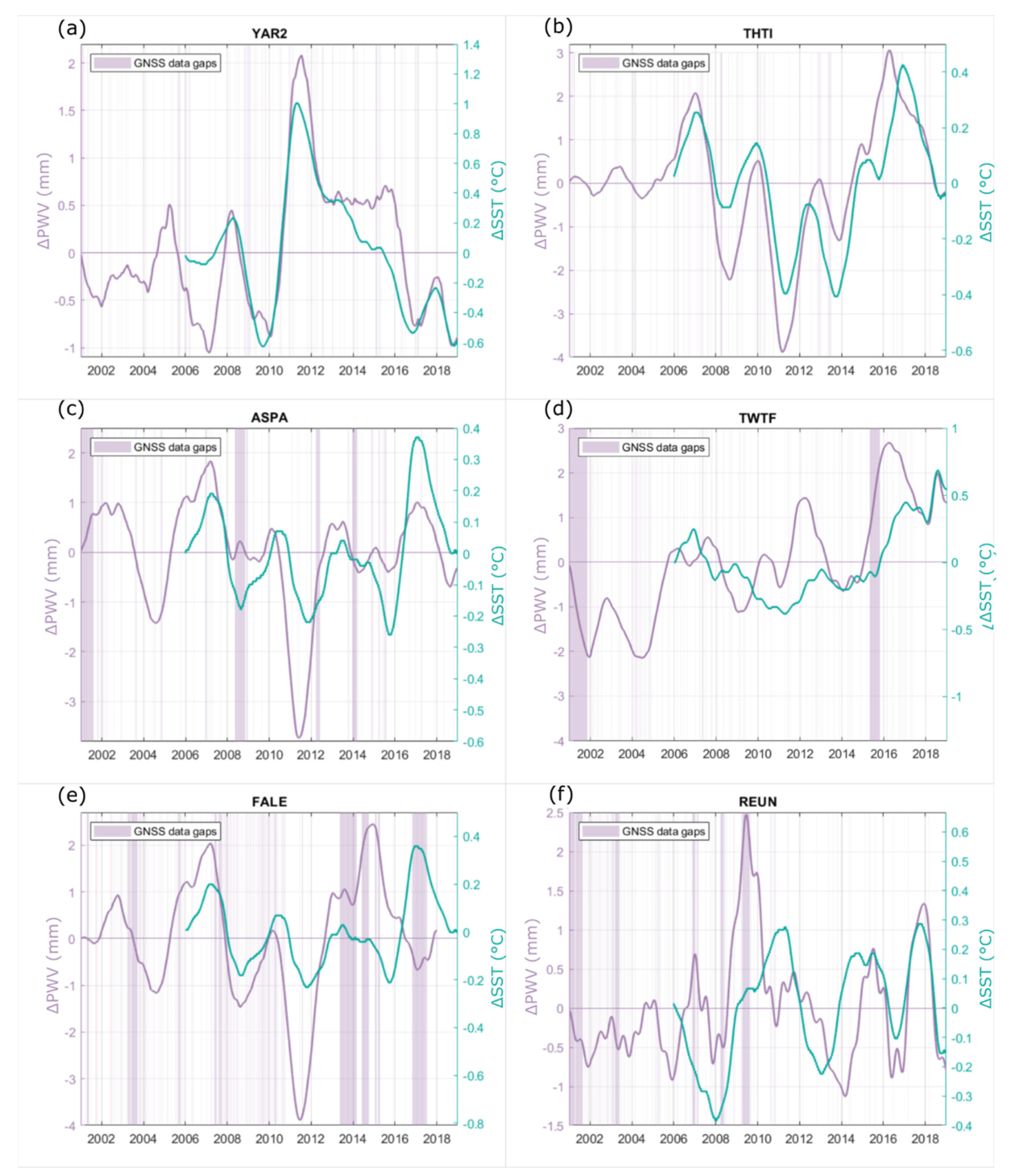
3.1.4. Non-Linear Trend Variability in Relation to Local SST
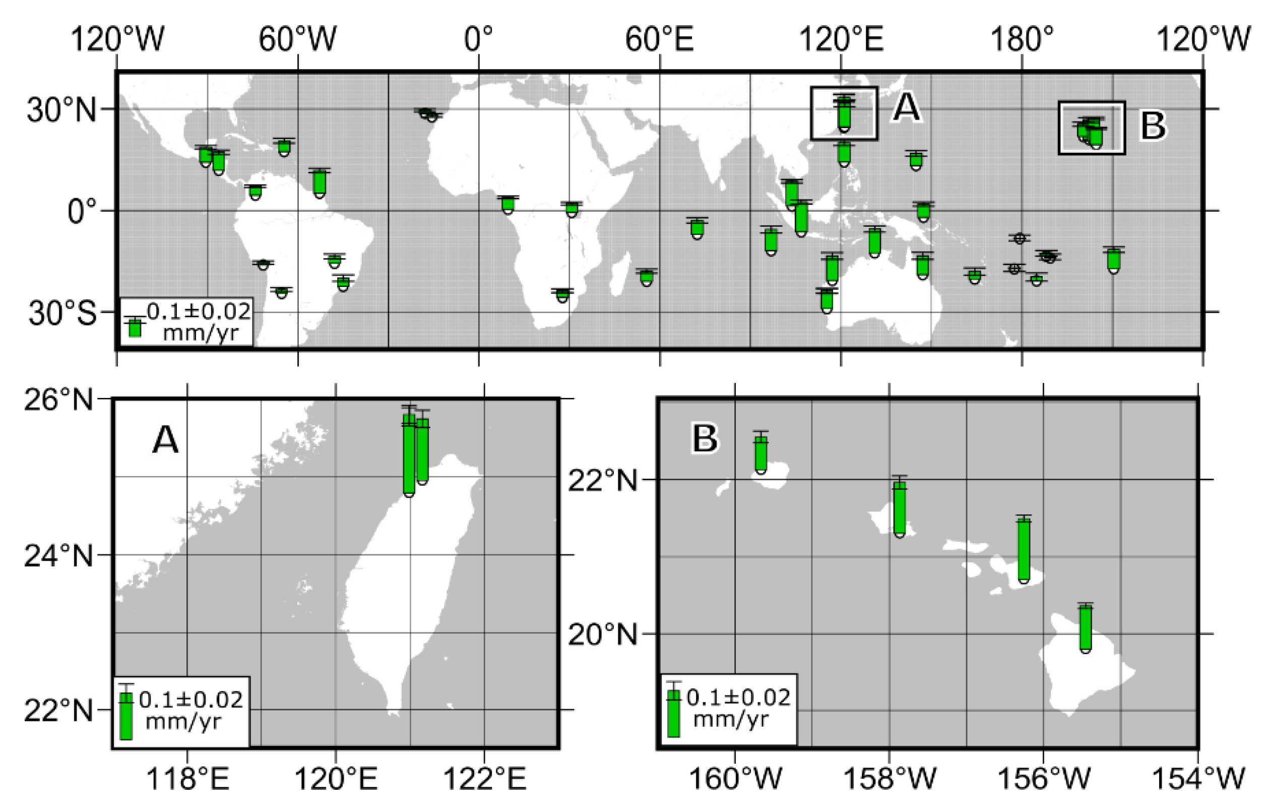
3.2. Linear Long-Term Variability
4. Discussion
5. Conclusions
Author Contributions
Funding
Institutional Review Board Statement
Informed Consent Statement
Data Availability Statement
Acknowledgments
Conflicts of Interest
Appendix A

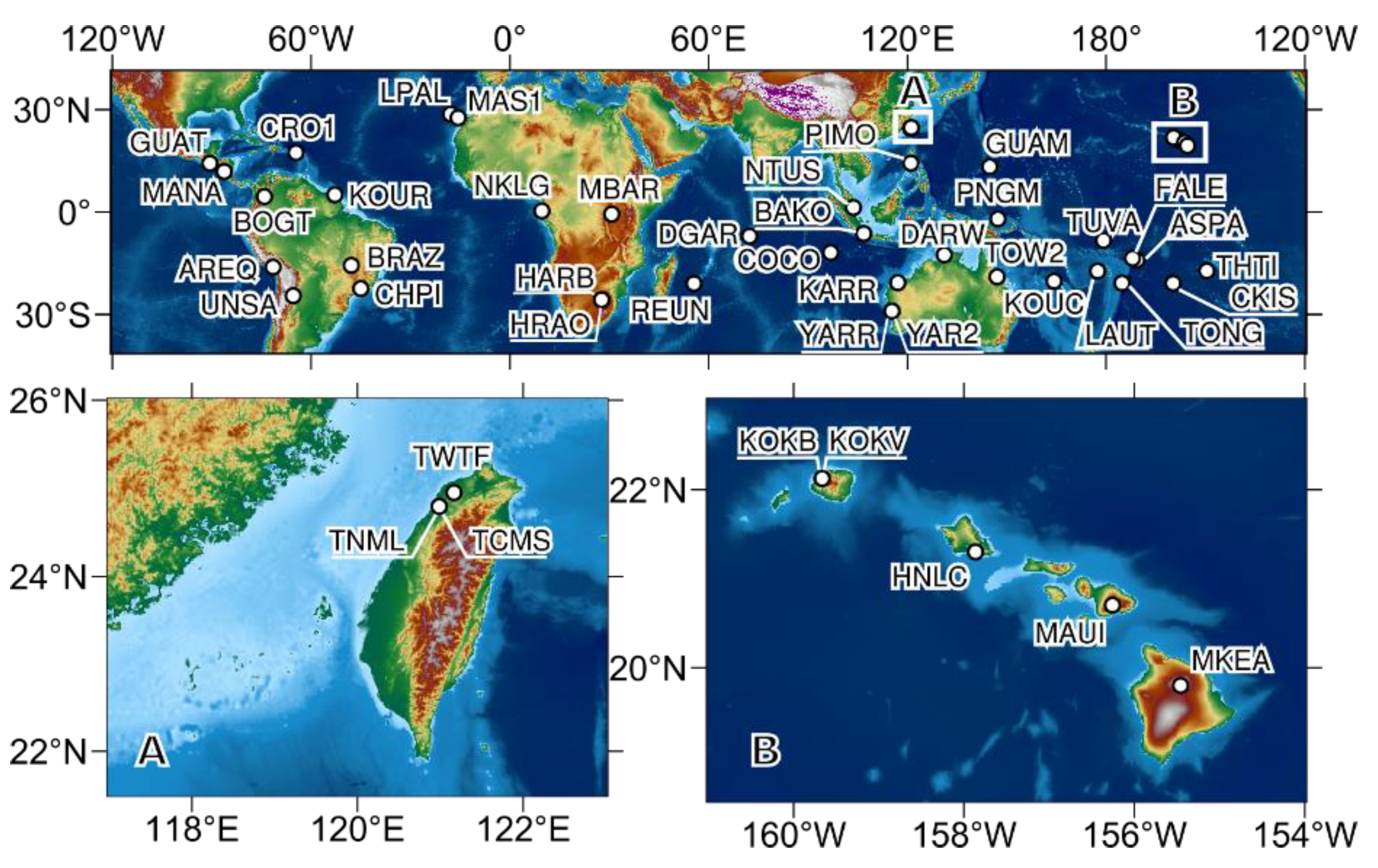
| Site | Location | Longitude [°] | Latitude [°] | Altitude [m] |
|---|---|---|---|---|
| AREQ | Arequipa, Peru | −71.49 | −16.47 | 2449.1 |
| ASPA | Pago Pago, United States | −170.72 | −14.33 | 21.1 |
| BAKO | Cibinong, Indonesia | 106.85 | −6.49 | 139.8 |
| BOGT | Bogota, Colombia | −74.08 | 4.64 | 2553.9 |
| BRAZ | Brasilia, Brazil | −47.88 | −15.95 | 1118.6 |
| CHPI | Cachoeira Paulista, Brazil | −44.99 | −22.69 | 620.8 |
| COCO | Cocos (Keeling) Island, Australia | 96.83 | −12.19 | 3.4 |
| CRO1 | Christiansted, Virgin Islands, United States | −64.58 | 17.76 | 12.2 |
| DARW | Darwin, Australia | 131.13 | −12.84 | 74.7 |
| DGAR | Diego Garcia Island, United Kingdom | 72.37 | −7.27 | 9.1 |
| FALE | Faleolo, Samoa | −172.00 | −13.83 | 9.7 |
| GUAM | Dededo, Guam | 144.87 | 13.59 | 146.4 |
| GUAT | Guatemala City, Guatemala | −90.52 | 14.59 | 1517.3 |
| HARB | Pretoria, South Africa | 27.71 | −25.89 | 1532.8 |
| HNLC | Honolulu, United States | −157.86 | 21.30 | 6.3 |
| HRAO | Krugersdorp, South Africa | 27.69 | −25.89 | 1388.9 |
| KARR | Karratha, Australia | 117.10 | −20.98 | 116.7 |
| KOKB | Kokee Park, Waimea, United States | −159.66 | 22.13 | 1150.5 |
| KOKV | Kokee Park, Waimea, United States | −159.66 | 22.13 | 1150.5 |
| KOUC | Koumac, New Caledonia | 164.29 | −20.56 | 23.7 |
| KOUR | Kourou, French Guiana | −52.81 | 5.25 | 8.7 |
| LAUT | Lautoka, Fiji | 177.45 | −17.61 | 31.7 |
| LPAL | Rogue de losMuchachos, Spain | −17.89 | 28.76 | 2207.0 |
| MANA | Managua, Nicaragua | −86.25 | 12.15 | 66.4 |
| MAS1 | Maspalomas, Spain | −15.63 | 27.76 | 197.2 |
| MAUI | Haleakala, Maui, United States | −156.26 | 20.71 | 3044.1 |
| MBAR | Mbarara, Uganda | 30.74 | −0.60 | 1349.6 |
| MKEA | Mauna Kea, United States | −155.46 | 19.80 | 3728.4 |
| NKLG | Libreville, Gabon | 9.67 | 0.35 | 21.5 |
| NTUS | Singapore, Singapore | 103.68 | 1.35 | 71.6 |
| PIMO | Quezon City, Philippines | 121.08 | 14.64 | 51.4 |
| PNGM | Lombrum, Papua New Guinea | 147.37 | −2.04 | 38.7 |
| REUN | Le Tampon, France | 55.57 | −21.21 | 1552.2 |
| TCMS | Hsinchu, Taiwan | 120.99 | 24.80 | 58.4 |
| THTI | Papeete, French Polynesia | −149.61 | −17.58 | 90.8 |
| TNML | Hsinchu, Taiwan | 120.99 | 24.80 | 57.0 |
| TONG | Nuku’alofa, Tonga | −175.18 | −21.14 | 3.7 |
| TOW2 | Cape Ferguson, Australia | 147.06 | −19.27 | 30.3 |
| TUVA | Funafuti, Tuvalu | 179.20 | −8.53 | 3.6 |
| TWTF | Taoyuan, Taiwan | 121.16 | 24.95 | 184.1 |
| UNSA | Salta, Argentina | −65.41 | −24.73 | 1224.4 |
| YAR2 | Yarragadee, Australia | 115.35 | −29.05 | 267.0 |
| YARR | Yarragadee, Australia | 115.35 | −29.05 | 267.1 |
References
- Ramage, C.S. Role of a Tropical “Maritime Continent” in the Atmospheric Circulation. Mon. Weather Rev. 1968, 96, 365–370. [Google Scholar] [CrossRef] [Green Version]
- Yamanaka, M.D.; Ogino, S.Y.; Wu, P.M.; Jun-Ichi, H.; Mori, S.; Matsumoto, J.; Syamsudin, F. Maritime Continent Coastlines Controlling Earth’s Climate. Prog. Earth Planet. Sci. 2018, 5, 21. [Google Scholar] [CrossRef]
- Barnett, T.P.; Pierce, D.W.; Latif, M.; Dommenget, D.; Saravanan, R. Interdecadal Interactions between the Tropics and Midlatitudes in the Pacific Basin. Geophys. Res. Lett. 1999, 26, 615–618. [Google Scholar] [CrossRef] [Green Version]
- Yeh, S.W.; Cai, W.; Min, S.K.; McPhaden, M.J.; Dommenget, D.; Dewitte, B.; Collins, M.; Ashok, K.; An, S.I.; Yim, B.Y.; et al. ENSO Atmospheric Teleconnections and Their Response to Greenhouse Gas Forcing. Rev. Geophys. 2018, 56, 185–206. [Google Scholar] [CrossRef]
- McPhaden, M.J.; Zebiak, S.E.; Glantz, M.H. ENSO as an Integrating Concept in Earth Science. Science 2006, 314, 1740–1745. [Google Scholar] [CrossRef] [Green Version]
- Luo, J.J.; Masson, S.; Behera, S.K.; Yamagata, T. Extended ENSO Predictions Using a Fully Coupled Ocean-Atmosphere Model. J. Clim. 2008, 21, 84–93. [Google Scholar] [CrossRef]
- Collins, D.; Power, S.B.; Sen Gupta, A.R. Observed Climate Variability and Trends. In Climate Change in the Pacific: Scientific Assessment and New Research; Cambers, G., Hennessy, H., Power, S., Eds.; CSIRO: Canberra, Australia, 2011; Volume 1, pp. 51–77. [Google Scholar]
- Trenberth, K.E.; Branstator, G.W.; Karoly, D.; Kumar, A.; Lau, N.-C.; Ropelewski, C. Progress during TOGA in Understanding and Modeling Global Teleconnections Associated with Tropical Sea Surface Temperatures. J. Geophys. Res. Ocean. 1998, 103, 14291–14324. [Google Scholar] [CrossRef]
- Turner, J. The El Niño-Southern Oscillation and Antarctica. Int. J. Climatol. 2004, 24, 1–31. [Google Scholar] [CrossRef] [Green Version]
- Yuan, X.; Kaplan, M.R.; Cane, M.A. The Interconnected Global Climate System-a Review of Tropical-Polar Teleconnections. J. Clim. 2018, 31, 5765–5792. [Google Scholar] [CrossRef]
- Hansen, J.; Lacis, A.; Rind, D.; Russell, G.; Stone, P.; Fung, I.; Ruedy, R.; Lerner, J. Climate Sensitivity: Analysis of Feedback Mechanisms. In Climate Processes and Climate Sensitivity; Hansen, J., Takahashi, T., Eds.; American Geophysical Union: Washington, DC, USA, 1984; Volume 29, pp. 130–163. [Google Scholar] [CrossRef] [Green Version]
- IPCC. Climate Change 2007: Synthesis Report. In Contribution of Working Groups I, II and III to the Fourth Assessment Report of the Intergovernmental Panel on Climate Change; Pachauri, R., Reisinger, A., Eds.; IPCC: Geneva, Switzerland, 2007. [Google Scholar]
- Dessler, A.E.; Zhang, Z.; Yang, P. Water-Vapor Climate Feedback Inferred from Climate Fluctuations, 2003–2008. Geophys. Res. Lett. 2008, 35. [Google Scholar] [CrossRef] [Green Version]
- Zhang, L.; Wu, L.; Gan, B. Modes and Mechanisms of Global Water Vapor Variability over the Twentieth Century. J. Clim. 2013, 26, 5578–5593. [Google Scholar] [CrossRef]
- Kiehl, J.T.; Trenberth, K.E. Earth’s Annual Global Mean Energy Budget. Bull. Am. Meteorol. Soc. 1997, 78, 197–208. [Google Scholar] [CrossRef] [Green Version]
- McGrath, R.; Semmler, T.; Sweeney, C.; Wang, S. Impact of Balloon Drift Errors in Radiosonde Data on Climate Statistics. J. Clim. 2006, 19, 3430–3442. [Google Scholar] [CrossRef]
- Seidel, D.J.; Sun, B.; Pettey, M.; Reale, A. Global Radiosonde Balloon Drift Statistics. J. Geophys. Res. 2011, 116, D07102. [Google Scholar] [CrossRef] [Green Version]
- Ferreira, A.P.; Nieto, R.; Gimeno, L. Completeness of Radiosonde Humidity Observations Based on the Integrated Global Radiosonde Archive. Earth Syst. Sci. Data 2019, 11, 603–627. [Google Scholar] [CrossRef] [Green Version]
- Baranowski, D.B.; Waliser, D.E.; Jiang, X.; Ridout, J.A.; Flatau, M.K. Contemporary GCM Fidelity in Representing the Diurnal Cycle of Precipitation Over the Maritime Continent. J. Geophys. Res. Atmos. 2019, 124, 747–769. [Google Scholar] [CrossRef]
- Nesbitt, S.W.; Zipser, E.J. The Diurnal Cycle of Rainfall and Convective Intensity According to Three Years of TRMM Measurements. J. Clim. 2003, 16, 1456–1475. [Google Scholar] [CrossRef] [Green Version]
- Yoneyama, K.; Zhang, C. Years of the Maritime Continent. Geophys. Res. Lett. 2020, 47, e2020GL087182. [Google Scholar] [CrossRef]
- Webster, P.J.; Lukas, R. TOGA COARE: The Coupled Ocean–Atmosphere Response Experiment. Bull. Am. Meteorol. Soc. 1992, 73, 1377–1416. [Google Scholar] [CrossRef] [Green Version]
- Bell, G.D.; Basist, A.N. The Global Climate of December 1992–February 1993. Part I: Warm ENSO Conditions Continue in the Tropical Pacific; California Drought Abates. J. Clim. 1994, 7, 1581–1605. [Google Scholar] [CrossRef]
- Gutzler, D.S.; Kiladis, G.N.; Meekl, O.A.; Weickmann, K.M.; Wheeler, M. The Global Climate of December 1992–February 1993. Part II: Large-Scale Variability across the Tropical Western Pacific during TOGA COARE. J. Clim. 1994, 7, 1606–1622. [Google Scholar] [CrossRef]
- Dole, R.M.; Spackman, J.R.; Newman, M.; Compo, G.P.; Smith, C.A.; Hartten, L.M.; Barsugli, J.J.; Webb, R.S.; Hoerling, M.P.; Cifelli, R.; et al. Advancing Science and Services during the 2015/16 El Niño: The NOAA El Niño Rapid Response Field Campaign. Bull. Am. Meteorol. Soc. 2018, 99, 975–1001. [Google Scholar] [CrossRef] [Green Version]
- Bevis, M.; Businger, S.; Herring, T.A.; Rocken, C.; Anthes, R.A.; Ware, R.H. GPS Meteorology: Remote Sensing of Atmospheric Water Vapor Using the Global Positioning System. J. Geophys. Res. 1992, 97, 15787–15801. [Google Scholar] [CrossRef]
- Nykiel, G.; Figurski, M.; Baldysz, Z. Analysis of GNSS Sensed Precipitable Water Vapour and Tropospheric Gradients during the Derecho Event in Poland of 11th August 2017. J. Atmos. Sol. Terr. Phys. 2019, 193, 105082. [Google Scholar] [CrossRef]
- Hagemann, S.; Bengtsson, L.; Gendt, G. On the Determination of Atmospheric Water Vapor from GPS Measurements. J. Geophys. Res. D Atmos. 2003, 108. [Google Scholar] [CrossRef] [Green Version]
- Morland, J.; Collaud Coen, M.; Hocke, K.; Jeannet, P.; Mätzler, C. Tropospheric Water Vapour above Switzerland over the Last 12 Years. Atmos. Chem. Phys. 2009, 9, 5975–5988. [Google Scholar] [CrossRef] [Green Version]
- Guerova, G.; Jones, J.; Douša, J.; Dick, G.; De Haan, S.; Pottiaux, E.; Bock, O.; Pacione, R.; Elgered, G.; Vedel, H.; et al. Review of the State of the Art and Future Prospects of the Ground-Based GNSS Meteorology in Europe. Atmos. Meas. Tech. 2016, 9, 5385–5406. [Google Scholar] [CrossRef] [Green Version]
- Jones, J.; Guerova, G.; Douša, J.; Dick, G.; de Haan, S.; Pottiaux, E.; Bock, O.; Pacione, R.; van Malderen, R. Advanced GNSS Tropospheric Products for Monitoring Severe Weather Events and Climate; Jones, J., Guerova, G., Douša, J., Dick, G., de Haan, S., Pottiaux, E., Bock, O., Pacione, R., van Malderen, R., Eds.; Springer Nature Switzerland AG: Berlin/Heidelberg, Germany, 2000. [Google Scholar] [CrossRef]
- Gradinarsky, L.P.; Johansson, J.M.; Bouma, H.R.; Scherneck, H.G.; Elgered, G. Climate Monitoring Using GPS. Phys. Chem. Earth 2002, 27, 335–340. [Google Scholar] [CrossRef]
- Baldysz, Z.; Nykiel, G.; Figurski, M.; Araszkiewicz, A. Assessment of the Impact of GNSS Processing Strategies on the Long-Term Parameters of 20 Years IWV Time Series. Remote Sens. 2018, 10, 496. [Google Scholar] [CrossRef] [Green Version]
- Vey, S.; Dietrich, R.; Rülke, A.; Fritsche, M.; Steigenberger, P.; Rothacher, M. Validation of Precipitable Water Vapor within the Ncep/Doe Reanalysis Using Global Gps Observations from One Decade. J. Clim. 2010, 23, 1675–1695. [Google Scholar] [CrossRef]
- Bock, O.; Willis, P.; Wang, J.; Mears, C. A High-Quality, Homogenized, Global, Long-Term (1993–2008) DORIS Precipitable Water Data Set for Climate Monitoring and Model Verification. J. Geophys. Res. Atmos. 2014, 119, 7209–7230. [Google Scholar] [CrossRef]
- Chen, B.; Liu, Z. Global Water Vapor Variability and Trend from the Latest 36 Year (1979 to 2014) Data of ECMWF and NCEP Reanalyses, Radiosonde, GPS, and Microwave Satellite. J. Geophys. Res. Atmos. 2016, 121, 11442–11462. [Google Scholar] [CrossRef]
- Ning, T.; Wickert, J.; Deng, Z.; Heise, S.; Dick, G.; Vey, S.; Schöne, T. Homogenized Time Series of the Atmospheric Water Vapor Content Obtained from the GNSS Reprocessed Data. J. Clim. 2016, 29, 2443–2456. [Google Scholar] [CrossRef]
- Parracho, A.C.; Bock, O.; Bastin, S. Global IWV Trends and Variability in Atmospheric Reanalyses and GPS Observations. Atmos. Chem. Phys. 2018, 18, 16213–16237. [Google Scholar] [CrossRef] [Green Version]
- Sohn, D.H.; Cho, J. Trend Analysis of GPS Precipitable Water Vapor above South Korea over the Last 10 Years. J. Astron. Space Sci. 2010, 27, 231–238. [Google Scholar] [CrossRef] [Green Version]
- Ning, T.; Elgered, G. Trends in the Atmospheric Water Vapor Content from Ground-Based GPS: The Impact of the Elevation Cutoff Angle. IEEE J. Sel. Top. Appl. Earth Obs. Remote Sens. 2012, 5, 744–751. [Google Scholar] [CrossRef] [Green Version]
- Bianchi, C.E.; Mendoza, L.P.O.; Fernández, L.I.; Natali, M.P.; Meza, A.M.; Moirano, J.F. Multi-Year GNSS Monitoring of Atmospheric IWV over Central and South America for Climate Studies. Ann. Geophys. 2016, 34, 623–639. [Google Scholar] [CrossRef] [Green Version]
- Saastamoinen, J. Atmospheric Correction for the Troposphere and Stratosphere in Radio Ranging Satellites. In The Use of Artificial Satellites for Geodesy; Henriksen, S.W., Mancini, A., Chovitz, B.H., Eds.; American Geophysical Union (AGU): Washington, DC, USA, 1972; pp. 247–251. [Google Scholar] [CrossRef]
- Bevis, M.; Businger, S.; Chiswell, S.; Herring, T.A.; Anthes, R.A.; Rocken, C.; Ware, R.H. GPS Meteorology: Mapping Zenith Wet Delays onto Precipitable Water. J. Appl. Meteorol. 1994, 33, 379–386. [Google Scholar] [CrossRef]
- Baldysz, Z.; Nykiel, G. Improved Empirical Coefficients for Estimating Water Vapor Weighted Mean Temperature over Europe for GNSS Applications. Remote Sens. 2019, 11, 1995. [Google Scholar] [CrossRef] [Green Version]
- Johnston, G.; Riddell, A.; Hausler, G. The International GNSS Service. In Springer Handbook of Global Navigation Satellite Systems; Teunissen, P.J., Montenbruck, O., Eds.; Springer Nature Switzerland AG: Berlin/Heidelberg, Germany, 2017; pp. 967–982. [Google Scholar] [CrossRef]
- Dach, R.; Lutz, S.; Walser, P.; Fridez, P. (Eds.) Bernese GNSS Software Version 5.2; University of Bern, Bern Open Publishing: Bern, Switzerland, 2015. [Google Scholar] [CrossRef]
- Steigenberger, P.; Lutz, S.; Dach, R.; Schaer, S.; Jäggi, A. CODE Repro2 Product Series for the IGS; Astronomical Institute, University of Bern: Bern, Switzerland, 2014. [Google Scholar] [CrossRef]
- Boehm, J.; Werl, B.; Schuh, H. Troposphere Mapping Functions for GPS and Very Long Baseline Interferometry from European Centre for Medium-Range Weather Forecasts Operational Analysis Data. J. Geophys. Res. Solid Earth 2006, 111. [Google Scholar] [CrossRef]
- Chen, G.; Herring, T.A. Effects of Atmospheric Azimuthal Asymmetry on the Analysis of Space Geodetic Data. J. Geophys. Res. Solid Earth 1997, 102, 20489–20502. [Google Scholar] [CrossRef]
- Hersbach, H.; Bell, B.; Berrisford, P.; Hirahara, S.; Horányi, A.; Muñoz-Sabater, J.; Nicolas, J.; Peubey, C.; Radu, R.; Schepers, D.; et al. The ERA5 Global Reanalysis. Q. J. R. Meteorol. Soc. 2020, 146, 1999–2049. [Google Scholar] [CrossRef]
- GHRSST. Group for High Resolution Sea Surface Temperature. (GHRSST)|PO.DAAC/JPL/NASA. Available online: https://www.usgodae.org/ftp/outgoing/fnmoc/models/ghrsst/ (accessed on 20 November 2020).
- Golyandina, N.; Nekrutkin, V.; Zhigljavsky, A. Analysis of Time Series Structure: SSA and Related Techniques; Chapman & Hall/CRC: New York, NY, USA, 2001. [Google Scholar]
- Ghil, M.; Allen, M.R.; Dettinger, M.D.; Ide, K.; Kondrashov, D.; Mann, M.E.; Robertson, A.W.; Saunders, A.; Tian, Y.; Varadi, F.; et al. Advanced Spectral Methods for Climatic Time Series. Rev. Geophys. 2002, 40, 1–41. [Google Scholar] [CrossRef] [Green Version]
- Broomhead, D.S.; King, G.P. Extracting Qualitative Dynamics from Experimental Data. Phys. D Nonlinear Phenom. 1986, 20, 217–236. [Google Scholar] [CrossRef]
- Kondrashov, D.; Ghil, M. Spatio-Temporal Filling of Missing Points in Geophysical Data Sets. Nonlinear Process. Geophys. 2006, 13, 151–159. [Google Scholar] [CrossRef] [Green Version]
- Hoseini, M.; Alshawaf, F.; Nahavandchi, H.; Dick, G.; Wickert, J. Towards a Zero-Difference Approach for Homogenizing GNSS Tropospheric Products. GPS Solut. 2020, 24, 8. [Google Scholar] [CrossRef]
- Wolter, K.; Timlin, M.S. El Niño/Southern Oscillation Behaviour since 1871 as Diagnosed in an Extended Multivariate ENSO Index (MEI.Ext). Int. J. Climatol. 2011, 31, 1074–1087. [Google Scholar] [CrossRef]
- Wang, X.; Zhang, K.; Wu, S.; Li, Z.; Cheng, Y.; Li, L.; Yuan, H. The Correlation between GNSS-Derived Precipitable Water Vapor and Sea Surface Temperature and Its Responses to El Niño–Southern Oscillation. Remote Sens. Environ. 2018, 216, 1–12. [Google Scholar] [CrossRef]
- Smith, I.; Moise, A.; Inape, K.; Murphy, B.; Colman, R.; Power, S.; Chung, C. ENSO-Related Rainfall Changes over the New Guinea Region. J. Geophys. Res. Atmos. 2013, 118, 10665–10675. [Google Scholar] [CrossRef]
- Meehl, G.A.; Arblaster, J.M. The Tropospheric Biennial Oscillation and Asian-Australian Monsoon Rainfall. J. Clim. 2002, 15, 722–744. [Google Scholar] [CrossRef]
- Jourdain, N.C.; Gupta, A.S.; Taschetto, A.S.; Ummenhofer, C.C.; Moise, A.F.; Ashok, K. The Indo-Australian Monsoon and Its Relationship to ENSO and IOD in Reanalysis Data and the CMIP3/CMIP5 Simulations. Clim. Dyn. 2013, 41, 3073–3102. [Google Scholar] [CrossRef] [Green Version]
- Murphy, B.F.; Power, S.B.; Mcgree, S. The Varied Impacts of El Niño-Southern Oscillation on Pacific Island Climates. J. Clim. 2014, 27, 4015–4036. [Google Scholar] [CrossRef]
- Chu, P.S.; Chen, H. Interannual and Interdecadal Rainfall Variations in the Hawaiian Islands. J. Clim. 2005, 18, 4796–4813. [Google Scholar] [CrossRef] [Green Version]
- NOAA National Centers for Environmental Information. State of the Climate: National Climate Report for Annual 2018; NOAA National Centers for Environmental Information: Asheville, NC, USA, 2019. [Google Scholar]
- NOAA National Centers for Environmental Information. Drought for Annual 2010; NOAA National Centers for Environmental Information: Asheville, NC, USA, 2011. [Google Scholar]
- Di Lorenzo, E.; Schneider, N.; Cobb, K.M.; Franks, P.J.S.; Chhak, K.; Miller, A.J.; McWilliams, J.C.; Bograd, S.J.; Arango, H.; Curchitser, E.; et al. North Pacific Gyre Oscillation Links Ocean Climate and Ecosystem Change. Geophys. Res. Lett. 2008, 35. [Google Scholar] [CrossRef] [Green Version]
- Ashok, K.; Guan, Z.; Yamagata, T. A Look at the Relationship between the ENSO and the Indian Ocean Dipole. J. Meteorol. Soc. Jpn. 2003, 81, 41–56. [Google Scholar] [CrossRef] [Green Version]
- Behera, S.K.; Luo, J.J.; Masson, S.; Rao, S.A.; Sakuma, H.; Yamagata, T. A CGCM Study on the Interaction between IOD and ENSO. J. Clim. 2006, 19, 1688–1705. [Google Scholar] [CrossRef]
- Stuecker, M.F.; Timmermann, A.; Jin, F.F.; Chikamoto, Y.; Zhang, W.; Wittenberg, A.T.; Widiasih, E.; Zhao, S. Revisiting ENSO/Indian Ocean Dipole Phase Relationships. Geophys. Res. Lett. 2017, 44, 2481–2492. [Google Scholar] [CrossRef]
- Saji, N.H.; Yamagata, T. Possible Impacts of Indian Ocean Dipole Mode Events on Global Climate. Clim. Res. 2003, 25, 151–169. [Google Scholar] [CrossRef]
- Wainwright, C.M.; Finney, D.L.; Kilavi, M.; Black, E.; Marsham, J.H. Extreme Rainfall in East Africa, October 2019–January 2020 and Context under Future Climate Change. Weather 2020, 76, 26–31. [Google Scholar] [CrossRef]
- McBride, J.L.; Nicholls, N. Seasonal Relationships between Australian Rainfall and the Southern Oscillation. Mon. Weather Rev. 1983, 111, 1998–2004. [Google Scholar] [CrossRef]
- Gallego, D.; Garcia, R.; Hernandez, E.; Gimeno, L.; Ribera, P. An ENSO Signal in the North Atlantic Subtropical Area. Geophys. Res. Lett. 2001, 28, 2939–2942. [Google Scholar] [CrossRef]
- Sánchez-Benítez, A.; García-Herrera, R.; Vicente-Serrano, S.M. Revisiting Precipitation Variability, Trends and Drivers in the Canary Islands. Int. J. Climatol. 2017, 37, 3565–3576. [Google Scholar] [CrossRef]
- Enfield, D.B.; Mestas-Nuñez, A.M.; Mayer, D.A.; Cid-Serrano, L. How Ubiquitous Is the Dipole Relationship in Tropical Atlantic Sea Surface Temperatures? J. Geophys. Res. Ocean. 1999, 104, 7841–7848. [Google Scholar] [CrossRef]
- Mason, S.J. Sea-surface Temperature—South African Rainfall Associations, 1910–1989. Int. J. Climatol. 1995, 15, 119–135. [Google Scholar] [CrossRef] [Green Version]
- Masante, D.; McCormick, N.; Vogt, J.; Carmona-Moreno, C.; Cordano, E.; Ameztoy, I. Drought and Water Crisis in Southern Africa. Eur. Comm. 2018, 100, 111596. [Google Scholar] [CrossRef]
- Martinez, C.; Goddard, L.; Kushnir, Y.; Ting, M. Seasonal Climatology and Dynamical Mechanisms of Rainfall in the Caribbean. Clim. Dyn. 2019, 53, 825–846. [Google Scholar] [CrossRef] [Green Version]
- Enfield, D.B.; Mestas-Nuñez, A.M.; Trimble, P.J. The Atlantic Multidecadal Oscillation and Its Relation to Rainfall and River Flows in the Continental U.S. Geophys. Res. Lett. 2001, 28, 2077–2080. [Google Scholar] [CrossRef] [Green Version]
- Bureau of Meteorology. Record-Breaking La Niña Events: An Analysis of La Niña Life Cycle and the Impacts and Significance of the 2010-11 and 2011-12 La Niña Events in Australia; Bureau of Meteorology: Melb, Australia, 2012. [Google Scholar]
- Boening, C.; Willis, J.K.; Landerer, F.W.; Nerem, R.S.; Fasullo, J. The 2011 La Nia: So Strong, the Oceans Fell. Geophys. Res. Lett. 2012, 39. [Google Scholar] [CrossRef] [Green Version]
- Choy, S.; Wang, C.S.; Yeh, T.K.; Dawson, J.; Jia, M.; Kuleshov, Y. Precipitable Water Vapor Estimates in the Australian Region from Ground-Based GPS Observations. Adv. Meteorol. 2015, 2015, 956481. [Google Scholar] [CrossRef] [Green Version]
- Yeh, T.K.; Hong, J.S.; Wang, C.S.; Chen, C.H.; Chen, K.H.; Fong, C.T. Determining the Precipitable Water Vapor with Ground-Based GPS and Comparing Its Yearly Variation to Rainfall over Taiwan. Adv. Space Res. 2016, 57, 2496–2507. [Google Scholar] [CrossRef]
- Baldysz, Z.; Nykiel, G.; Araszkiewicz, A.; Figurski, M.; Szafranek, K. Comparison of GPS Tropospheric Delays Derived from Two Consecutive EPN Reprocessing Campaigns from the Point of View of Climate Monitoring. Atmos. Meas. Tech. 2016, 9, 4861–4877. [Google Scholar] [CrossRef] [Green Version]
- Bosser, P.; Bock, O.; Flamant, C.; Bony, S.; Speich, S. Integrated Water Vapour Content Retrievals from Ship-Borne GNSS Receivers during Eurec4a. Earth Syst. Sci. Data 2021, 13, 1499–1517. [Google Scholar] [CrossRef]
- Baldysz, Z.; Nykiel, G.; Figurski, M. Tropospheric Parameters Derived from the Selected IGS Stations in the Global Tropics for the Years 2001–2018; Gdańsk University of Technology: Gdansk, Poland, 2021. [Google Scholar] [CrossRef]
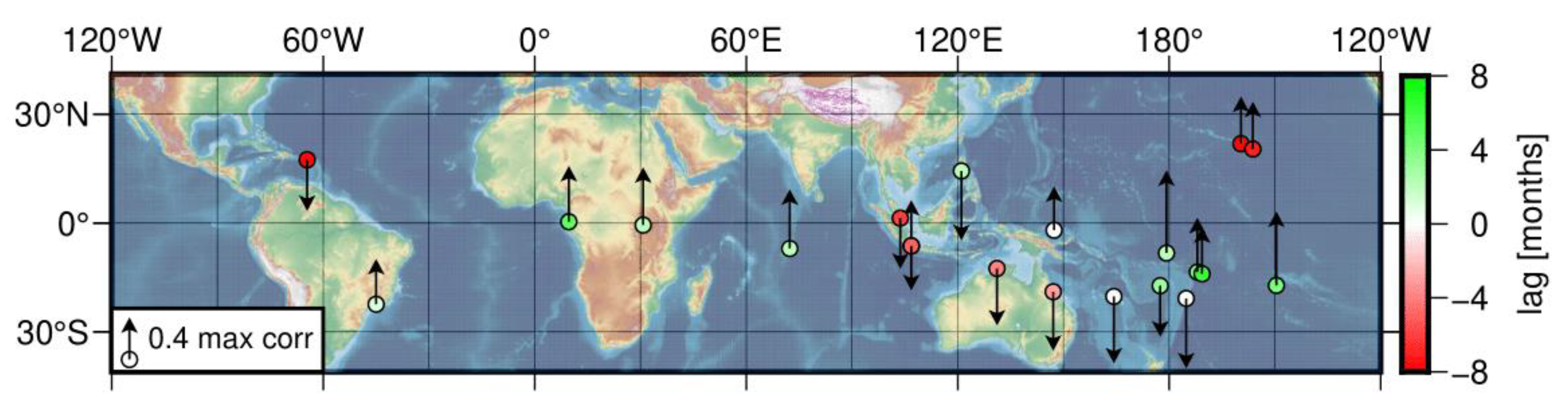
| Site | Cross-Correlation Coefficient | Lag [Months] | Site | Cross-Correlation Coefficient | Lag [Months] |
|---|---|---|---|---|---|
| TUVA | 0.78 | +2 | PNGM | 0.41 | 0 |
| THTI | 0.70 | +4 | BAKO | −0.42 | −5 |
| DGAR | 0.56 | +2 | NTUS | −0.48 | −6 |
| MBAR | 0.55 | +2 | LAUT | −0.48 | +3 |
| NKLG | 0.52 | +5 | CRO1 | −0.48 | −8 |
| FALE | 0.51 | +4 | DARW | −0.53 | −4 |
| MAUI | 0.44 | −7 | TOW2 | −0.56 | −3 |
| KOKB | 0.45 | −8 | KOUC | −0.63 | 0 |
| ASPA | 0.44 | +6 | PIMO | −0.66 | −2 |
| KOKV | 0.43 | −10 | TONG | −0.66 | 0 |
| CHPI | 0.42 | +1 |
| Site | SST Corr. | Climate Index | Site | SST Corr. | Climate Index |
|---|---|---|---|---|---|
| YAR2 | 0.87 | - | ASPA | 0.58 | MEI (p) |
| HNLC | 0.86 | NPGO (n) | MAUI | 0.55 | NPGO (n) |
| TUVA | 0.85 | MEI (p) | DARW | 0.54 | DMI_east (p) |
| TONG | 0.83 | MEI (n) | CHPI | 0.51 | - |
| COCO | 0.81 | DMI_east (p) | GUAM | 0.51 | - |
| MKEA | 0.81 | NPGO (p) | KOUR | 0.50 | CAR (p) |
| THTI | 0.80 | MEI (p) | NTUS | 0.50 | MEI (n) |
| BAKO | 0.76 | DMI_east (p) | TOW2 | 0.45 | MEI (n) |
| GUAT | 0.75 | CAR (p) | KOUC | 0.38 | MEI (n) |
| YARR | 0.75 | - | KARR | 0.36 | - |
| CRO1 | 0.73 | CAR (p) | MANA | 0.36 | CAR (p) |
| LAUT | 0.70 | MEI (n) | REUN | 0.36 | - |
| KOKB | 0.68 | NPGO (n) | IISC | 0.34 | - |
| LPAL | 0.68 | TNA (p) | FALE | 0.33 | MEI (p) |
| KOKV | 0.67 | NPGO (n) | TNML | 0.27 | - |
| DGAR | 0.66 | DMI_west (p) | TCMS | 0.25 | - |
| NKLG | 0.61 | CAR (p) | AREQ | 0.24 | - |
| MAS1 | 0.60 | TNA (p) | PIMO | −0.19 | MEI (n) |
| TWTF | 0.59 | - | PNGM | −0.26 | MEI (p) |
Publisher’s Note: MDPI stays neutral with regard to jurisdictional claims in published maps and institutional affiliations. |
© 2021 by the authors. Licensee MDPI, Basel, Switzerland. This article is an open access article distributed under the terms and conditions of the Creative Commons Attribution (CC BY) license (https://creativecommons.org/licenses/by/4.0/).
Share and Cite
Baldysz, Z.; Nykiel, G.; Latos, B.; Baranowski, D.B.; Figurski, M. Interannual Variability of the GNSS Precipitable Water Vapor in the Global Tropics. Atmosphere 2021, 12, 1698. https://doi.org/10.3390/atmos12121698
Baldysz Z, Nykiel G, Latos B, Baranowski DB, Figurski M. Interannual Variability of the GNSS Precipitable Water Vapor in the Global Tropics. Atmosphere. 2021; 12(12):1698. https://doi.org/10.3390/atmos12121698
Chicago/Turabian StyleBaldysz, Zofia, Grzegorz Nykiel, Beata Latos, Dariusz B. Baranowski, and Mariusz Figurski. 2021. "Interannual Variability of the GNSS Precipitable Water Vapor in the Global Tropics" Atmosphere 12, no. 12: 1698. https://doi.org/10.3390/atmos12121698
APA StyleBaldysz, Z., Nykiel, G., Latos, B., Baranowski, D. B., & Figurski, M. (2021). Interannual Variability of the GNSS Precipitable Water Vapor in the Global Tropics. Atmosphere, 12(12), 1698. https://doi.org/10.3390/atmos12121698