Abstract
Planetary-scale 4-day Kelvin-type waves at the cloud top of the Venus atmosphere have been reported from the 1980s, and their significance for atmospheric dynamics has been pointed out. However, these waves have not been reproduced in Venus atmospheric general circulation models (VGCMs). Recently, horizontal winds associated with the planetary-scale waves at the cloud top have been obtained from cloud images taken by cameras onboard Venus orbiters, which could enable us to clarify the structure and roles of Kelvin-type waves. In order to examine this possibility, our team carried out an idealized observing system simulation experiment (OSSE) with a data assimilation system which we developed. The wind velocity data provided by a CCSR/NIES (Center for Climate System Research/National Institute for Environmental Studies) VGCM where equatorial Kelvin-type waves were assumed below the cloud bottom was used as idealized observations. Results show that 4-day planetary-scale Kelvin-type waves are successfully reproduced if the wind velocity between 15° S and 15° N latitudes is assimilated every 6 h at 70 km altitude. It is strongly suggested that the Kelvin-type waves could be reproduced and investigated by the data assimilation with the horizontal wind data derived from Akatsuki ultraviolet images. The present results also contribute to planning future missions for understanding planetary atmospheres.
1. Introduction
In spite of the slow rotation of its solid globe, the atmosphere of Venus rotates much faster, with zonal winds of ~100 m/s at the cloud top altitude of ~70 km e.g., [1,2], which are called super rotation. At the cloud top, signals of planetary-scale Kelvin- and Rossby-type waves, which propagate faster and slower than the zonal flow with periods of ~4 and ~5 Earth days, respectively, have been reported by many observational studies e.g., [3,4,5,6,7]. At ~60 km, equatorial waves with periods of 3.5–8.4 days have been also observed [8]. Because Venus general circulation is considered to be strongly affected by these planetary-scale waves through momentum and heat transport, it is crucially important to understand the physical processes of these waves, such as generation, propagation, and dissipation. For example, the Gierasch mechanism [9,10] assumes that angular momentum is transported toward the equatorial region in order to generate and maintain the super rotation and the planetary-scale Kelvin-type waves observed in the equatorial region are one of the candidates. However, the observed equatorial Kelvin-type waves at the cloud top have not been reproduced so far in any Venusian atmospheric general circulation models (VGCMs).
Recently, Venus GCM named AFES-Venus [11] based on AFES (an atmospheric GCM for the Earth Simulator) [12] has been developed. Using realistic distribution of the solar heating and static stability, and starting from an idealized super-rotating flow, AFES-Venus reproduced the super rotation with planetary-scale waves [13,14], the polar vortex with so-called cold collar [15], the thermal tides [16], the thermal structure in the equatorial region [17], and the planetary-scale streak structure [18]. However, the Kelvin-type waves with a period of ~4 days at the cloud top are not reproduced, though waves with a longer period of ~6.2 days appear in the equatorial region below ~50 km [13]. On the other hand, CCSR/NIES (Center for Climate System Research/National Institute for Environmental Studies) VGCM, another Venus GCM different from AFES-Venus, reproduces the Kelvin-type waves with a period of ~4 days at the cloud top [19], though forcing of 5.5-day wave observed in near-infrared imaging [20] was assumed at the lowest level (~30 km) of the VGCM.
Data assimilation has been widely conducted for the Earth and Mars atmospheres, which is one of the best ways to reduce error between model results and observations e.g., [21]. Recently, the first data assimilation system for the Venus atmosphere named ALEDAS-V (AFES LETKF Data Assimilation System for Venus) has been developed [22] using Local Ensemble Transform Kalman Filter (LETKF) based on AFES-Venus, which enables us to improve structures of the thermal tide by using the wind velocity data derived from the Venus Monitoring Camera onboard the Venus Express (VMC/VEX) [23]. In addition, Sugimoto et al. [24] conducted observing system simulation experiments (OSSE) for radio occultation measurements among small satellites. Using several types of temperature observations, they successfully reproduced the cold collar in the cases assuming 2 or 3 small satellites.
In this study, we will conduct an idealized OSSE for observations with various wavelength cameras (e.g., infra-red, ultra-violet, so on) to reproduce Kelvin-type waves at the cloud top. The idealized observation data of wind velocity is created from CCSR/NIES VGCM [19], in which the equatorial Kelvin-type waves are reproduced at the cloud top by the wave forcing at the cloud bottom boundary. Sensitivity experiments to the observational altitude, latitudinal range, and frequency have been done, and the observation conditions necessary to reproduce 4-day Kelvin-type waves by the data assimilation will be investigated. This paper is organized as follows. Methods and models used in this study are described in Section 2. Results of 4-day Kelvin-type waves reproduction with several types of observations are presented in Section 3, followed by discussion and conclusion in Section 4 and Section 5.
2. Experiments
The dynamical core of AFES-Venus implements the primitive equations of a global, 3D, dry atmosphere. We set physical parameters to those on Venus. The latitude-longitude grids system is adopted and horizontal resolution is 128 times 64. We use 60 vertical layers with ~2 km intervals. Model top is set to 120 km. Profile of solar heating based on [25] is used. Newtonian cooling with coefficients based on [26] is used as a simple radiative transfer scheme. The vertical and horizontal eddy diffusions are used. The coefficient of vertical eddy diffusion is 0.15 m2/s. Second-order hyper viscosity is used for the horizontal eddy diffusion. Damping time is ~0.1 Earth day for the maximum wave number component. At the lowest level, Rayleigh friction is used as the surface friction. A sponge layer is also used in the upper atmosphere above 80 km. It acts only for eddy components and mean zonal flow is not decelerated by the sponge layer. There is no topography and planetary boundary layer. The simulation starts from zonal flow assuming idealized super rotation, which is balanced with a temperature field including low static stability layers, and spins up the general circulation for 4 Earth years from 1 January 2001. More details are described in the previous works [11,13]
Data assimilation is a method to make an accurate and reliable prediction by comparing data of forecast and observation. ALEDAS-V uses the AFES-Venus and LETKF [27]. AFES-Venus proceeds short time ensemble forecasts. We set ensemble members to 31. LETKF combines observations and ensemble forecasts to create an improved estimate (analysis). We set the assimilation cycle to 6 hourly intervals with 1 hourly observation window. Observation error is set to 3 m/s with an inflation size of 10% based on the previous works [22,23]. The localization parameters are 400 km in horizontal and in vertical, where P is pressure. We have examined the effect of these localization parameters in the previous work [22], showing that assimilation results are almost unchanged for their values of 200–800 km and 0.2–0.8. AFES-Venus forecasts 9 h, and ALEDAS-V uses simulated data between t = 3 and t = 9 h for the assimilation. Observations are inputted from t = 3 to t = 9 h if they are available, and LETKF outputs analysis at t = 6 h. Observation period is 1 month from January 1, 2005. Details are found in the previous works [22,23].
As mentioned above, the idealized wind observation data are provided from CCSR/NIES VGCM (cf. results of Exp. D in Ref. [19]), in which the 4-day equatorial Kelvin-type waves are reproduced at the cloud top. Horizontal resolution is 64 times 32 in latitude-longitude grids system. Note that this horizontal resolution is much lower than that of the observation data obtained by the Akatsuki orbiter, ~3 degree interval. We used covariance matrix including winds and temperature. Therefore, temperature is also updated so that its uncertainty will be small by the LETKF algorithm. It should be noted that CCSR/NIES VGCM uses 5.5-day wave forcing at the cloud bottom and reproduces mean zonal flow with strong mid-latitude jets (~160 m/s), which is largely different from that reproduced in AFES-Venus.
Prior to the OSSE experiments, we conducted a preliminary experiment in which horizontal winds with a different observational frequency were assimilated at several different altitudes. The results showed that the 4-day Kelvin-type waves were reproduced only if the horizontal winds were assimilated at 70 km because of model bias (Appendix A). Based on this preliminary result and the challenge of observations lower in the cloud deck, we limit the altitude to 70 km (Table 1). This choice is also consistent with that wind velocity derived from images of ultraviolet wavelength camera on the Akatsuki orbiter are available at this altitude. Next, we checked the assimilation frequency. The result indicated that the best assimilation frequency was once in 6 h. Therefore, we will focus on “h6” results mainly.

Table 1.
Cases of idealized wind observations for observing system simulation experiments. Idealized wind observations at 70 km are assumed to be derived from images of ultraviolet wavelength camera on the Akatsuki orbiter. Headings in the vertical column indicate latitudinal range of observations and headings in the horizontal row indicate frequency of observations. For example, z70l90h6 means, assimilating data is given within 90°S–90°N at every 6 h at 70 km altitude. In the bottom row, “frf” means free run forecast (without data assimilation) and “ym-dat” means the original CCSR/NIES VGCM [19] full data set used for idealized observation.
3. Results
In this section, results obtained from the OSSE are shown. Section 3.1 demonstrates zonal mean field for the basic state. Results of time evolution are displayed in Section 3.2, and the structure of Kelvin-type waves is extracted by composite means of horizontal sections in Section 3.3. Finally, necessary conditions for observation regarding the reproduction of Kelvin-type waves are examined in Section 3.4.
3.1. Zonal Mean Field
First, we will show mean zonal wind and temperature obtained by assimilating data of wind velocity at an altitude of 70 km (Figure 1). Strong jets predominate (~160 m/s) in mid-latitudes in the original CCSR/NIES VGCM [19] observation data (Figure 1a), while weak jets (~120 m/s) appear in mid-latitudes in the original AFES-Venus free run forecast where data is not assimilated, with almost uniform velocity in the equatorial region (Figure 1b). Hence, significant difference occurred in analysis between cases of the jets excluded assimilation (Figure 1c) and jets included assimilation (Figure 1d). The wind velocity in the equatorial region in Figure 1b,c are almost uniform at 70–75 km, while it is almost uniform at ~65 km in Figure 1d. This difference is most likely to be caused by using a wide range of latitude including the strong jets for data assimilation in Figure 1d. As a result, the strong jets had been reproduced in mid-latitudes, and angular momentum would be transported to the equator. Comparing these results, Figure 1c,d are similar to Figure 1a,b (i.e., free run forecast and idealized observation data), respectively.
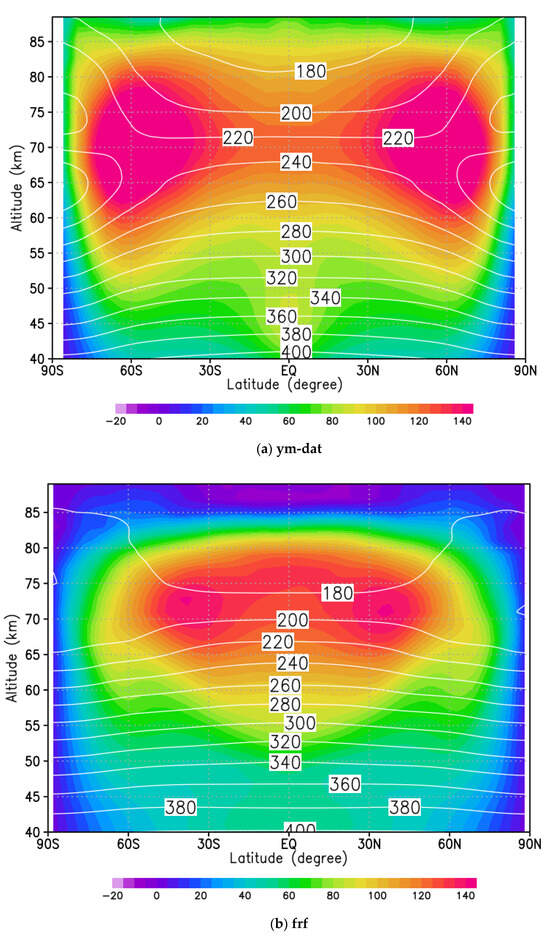
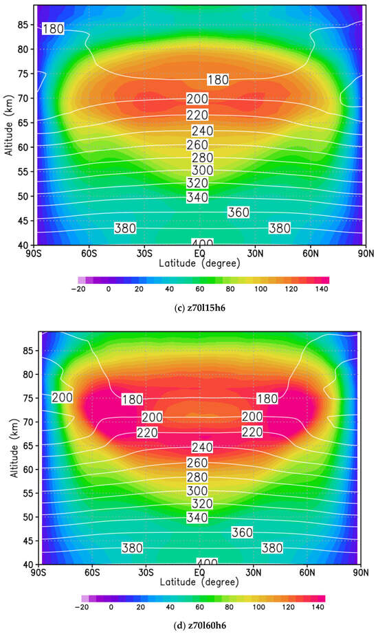
Figure 1.
Latitude-altitude cross sections of mean zonal wind (color) and temperature (contour) on 30 January 2005. (a) The original CCSR/NIES VGCM [19] observation data, (b) free run forecast of AFES-Venus, namely, data is not assimilated, while it is assimilated (analysis) each 6 h at 70 km altitude from 15° S–15° N in (c) and from 60° S–60° N in (d).
3.2. Time Evolution
In this subsection, the reproducibility of 4-day Kelvin-type waves was examined in multiple ways. Hovmöller diagrams show the effect of data assimilation (Figure 2), which visualize the zonal wind deviation from its time average in longitude-time cross-sections at the equator at 70 km altitude (Figure 2), the effect of data assimilation can be seen. In Figure 2, black arrows indicate almost 4-day phase velocity, namely, it is about 4-days from left to right of the arrow. Although the 4-day Kelvin-type waves are vague without assimilation (Figure 2a), they are clearly reproduced in the cases with assimilation (Figure 2b,c; analysis). It is noted that a westward slowly propagating wave with the wave number of 2 observed in all the cases is a semidiurnal thermal tide [16].

Figure 2.
Longitude-time cross sections of zonal wind deviation from its time average at 70 km altitude at the equator from 1 January 2005. Data is not assimilated in (a), namely, free run forecast of AFES-Venus, while it is assimilated (analysis) each 6 h at 70 km altitude from 15° S–15° N in (b) and from 60° S–60° N in (c). Black arrows indicate almost 4-day phase velocity from bottom left to upper right.
In order to investigate vertical structure and propagation of the Kelvin-type waves, zonal wind deviation from its 10-day running mean was visualized in time-altitude cross-sections at the equator (Figure 3). Black lines in Figure 3 indicate 70 km altitude. In Figure 3a, only ~5.5-day waves (about 5 to 6 cycles during a month) appear at 60–75 km levels. On the other hand, in Figure 3b,c (analysis), the 4-day Kelvin-type waves (about 7 to 8 cycles during a month) are reproduced at 70 km, and their structure extends from altitude 65 to 75 km. They also seem to propagate toward even upper altitude (~80 km).

Figure 3.
Time-altitude cross sections of zonal wind deviation from its 10-day running mean at the equator from 1 January 2005. Data is not assimilated in (a), namely, free run forecast of AFES-Venus, while it is assimilated (analysis) each 6 h at 70 km altitude from 15° S–15° N in (b) and from 60° S–60° N in (c). Black lines clarify an altitude of 70 km.
Finally, we examine horizontal propagation of the 4-day Kelvin-type waves by visualizing wind and temperature in a longitude-latitude cross-section; continuously for a period of 6 days for the case of z70l15h6 (Figure 4; analysis). The black lines in the panels indicate longitudes where directions of zonal wind change their signs in the equatorial region. The location of the two lines are almost the same (in 1 January and 5 January). Thus, the Kelvin-type waves are circulating Venus in about 4-days. See also for animations in 6 hourly periods from 1 to 30 January 2005, for the cases of z70l15h6 (analysis) and frf, respectively.
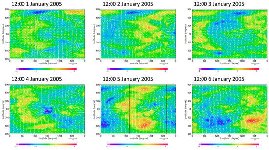
Figure 4.
Time variations of temperature (color) and wind velocity (vector) deviations from their zonal averages in latitude-longitude cross sections at 70 km for the case of z70l15h6 (analysis).
3.3. Composite Means
In order to derive the structure of the 4-day Kelvin-type waves, we carried out composite means by averaging successive 85 snapshots along with phase velocity of about 4 days (e.g., black line in Figure 2). Figure 5 represents composite means of horizontal sections at 70 km altitude of zonal wind, temperature, and meridional wind obtained for (Figure 5a) frf, free run forecast, (Figure 5b) z70l5h6, (Figure 5c) z70l15h6, and (Figure 5d) z70l30h6 (analysis) in which the Kelvin-type waves are relatively well reproduced. It is clearly shown that the wave number 1 component of zonal wind is predominant in equatorial region, which is symmetric to the equator without meridional wind, and corresponds to the Kelvin-type waves (Figure 5b–d). It is noted that this structure is never seen in frf (Figure 5a). Moreover, though only wind velocity was assimilated, a wave number 1 structure is induced in the temperature field around the equator, having a phase difference of 60° comparing to the zonal wind. This phase shift suggests that the Kelvin-type waves would propagate in the vertical direction. Temperature disturbances (with a 4-day period) with wave number 1 in mid-latitudes are interactions between Kelvin-type waves and Rossby-type waves embedded in mid-latitudes in the original AFES-Venus runs. A major difference in Figure 5 occurs at z70l30h6 (d). Despite the other two latitudinal range experiments, each physical value is relatively large. The cause is presumed that influence of mutual interactions between the 4-day Kelvin-type and Rossby-type waves in mid-latitudes had increased by setting a wide range of latitude (up to mid-latitude) for the data assimilation.
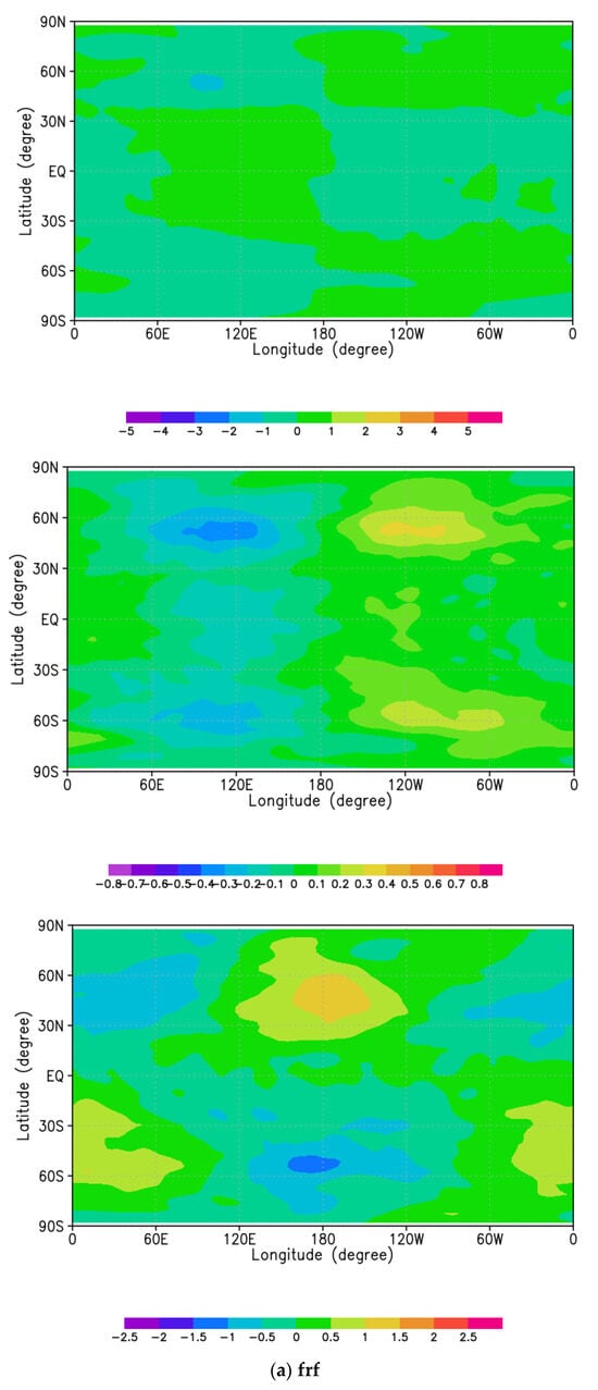
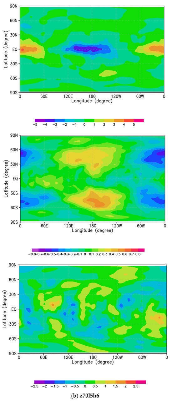
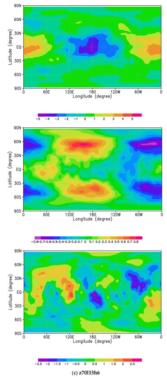
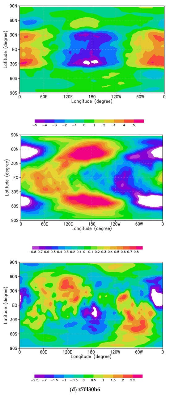
Figure 5.
Composite means of zonal wind (top panels), temperature (middle panels), and meridional wind (bottom panels) in latitude-longitude cross sections at 70 km for (a) frf, namely, free run forecast of AFES-Venus, and the cases of (b) z70l5h6, (c) z70l15h6 and (d) z70l30h6 (analysis). The total number of visualized data used for composite means is 85, with every data arranged equally in purpose of extracting equatorial Kelvin-type waves with about 4-day periodicity.
Figure 6 shows composite means of vertical sections of zonal wind (top panels) and temperature (bottom panels) in longitude-altitude sections at the equator obtained for (Figure 6a) frf, free run forecast, (Figure 6b) z70l5h6, (Figure 6c) z70l15h6 and (Figure 6d) z70l30h6 (analysis). Although wind velocity was assimilated only at 70 km altitude, the Kelvin-type waves extend vertically for about 10 km (65–75 km altitudes). Since the vertical localization at 70 km is ~O(102) m, which is smaller than a vertical grid interval, the vertical extension of Kelvin-type waves would be realistic. As shown in the horizontal structures, a wave number 1 structure is induced with a phase difference of 60° in the temperature field. It looks like the waves propagate vertically as seen in both the zonal wind and temperature fields, however, it is not clear especially in the temperature field for (Figure 6d).
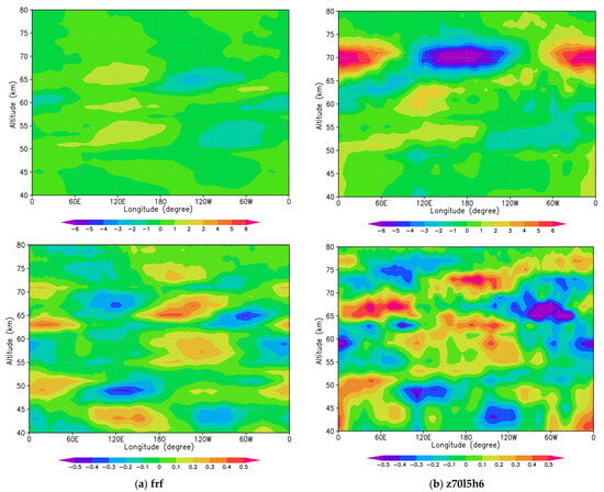
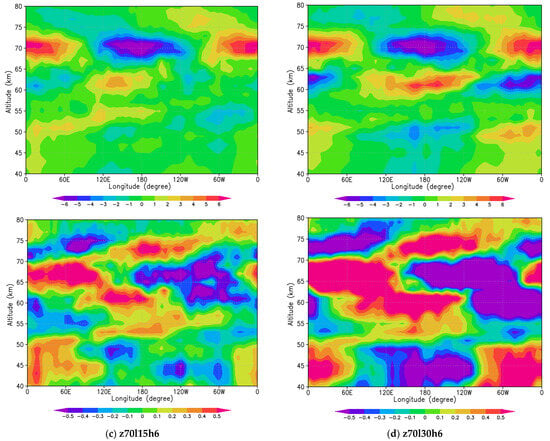
Figure 6.
Composite means of zonal wind (top panels) and temperature (bottom panels) in longitude-altitude sections at the equator obtained for (a) frf, namely, free run forecast of AFES-Venus, and the cases of (b) z70l5h6, (c) z70l15h6 and (d) z70l30h6 (analysis). The total number of successive data used for composite means is 85, with every data arranged equally in order to extract the equatorial Kelvin-type waves with about 4-day period.
3.4. Requirements for the Reproduction of Kelvin-Type Waves
In the previous section, composite means were carried out for the cases in which the Kelvin-type waves were successfully reproduced. In this section, we explore desirable observational conditions to reproduce the Kelvin-type waves. Figure 7a shows how Root-mean-square deviation (RMSD) depends on latitudinal ranges of assimilating data for cases with the same time interval of 6-h, which is defined by

Figure 7.
Root-mean-square deviation (RMSD) of zonal wind (analysis) from that of frf at 70 km calculated by Equation (1) from 1 January 2005. (a) Latitudinal dependency in case of assimilating data at the same time interval of 6 h. (b) Observation frequential dependency in case of assimilating data at the same latitudinal range of 15° S–15° N. (c) Longitude-time cross sections of zonal wind deviation from its time average at 70 km altitude at the equator from 1 January 2005 for z70l15h24 (analysis).
Here, indicates original values of frf, free run forecast whereas indicates assimilated values (analysis). N is the total number of horizontal grid points at 70 km. In the case of l60 (denoted by a purple line), RMSD increases with time significantly, supporting the hypothesis proposed in Figure 1 (i.e., in correspondence of wind velocity between Figure 1c,d). This result suggests that, since the basic wind distributions are quite different between the original CCSR/NIES VGCM (ym-dat [19]) and AFES-Venus, the wind distribution is drastically changed if the mid-latitudes jets are included for the data assimilation. In other cases, RMSDs are almost flat and stabilized. Therefore, we have to prepare observations with a limited latitudinal range (e.g., in the equatorial region) if there is a non-negligible discrepancy in mid-latitudes jets between observations and AFES-Venus.
Figure 7b shows how RMSD depends on observation frequencial dependency of assimilating data for cases with the same latitudinal range of 15° S–15° N. In the case of h6, RMSD increases gradually with time from half past a month, while RMSDs are almost stabilized in the other two cases (h12 and h24). However, the assimilation impact appears to be too large for the h12 and h24 cases because of low frequency, as suggested by the Hovmöller diagram for the h24 case (Figure 7c). It is noted that the assimilation impact oscillates quickly in the h12 and h24 cases (Figure 7b), because only 1/2 or 1/4 observations are taken within a cycle of analysis as compared with the h6 case. It is also confirmed that the reproduced structures of Kelvin-type waves are unclear in these two analyses (not shown). Therefore, at least 6-hourly observations will be needed to reproduce the Kelvin-type waves. We have also investigated the ensemble spread of each case and confirmed that z70l15h6 is the best choice among the cases (Appendix B).
4. Discussion
We will hereby discuss why the Kelvin-type waves are reproduced successfully in the case of z70l15h6 and is not in other cases. First, the equatorial Kelvin-type waves are reproduced only if the wind data is assimilated at 70 km altitude. If the wind data is assimilated at other levels, they cannot be reproduced. Since the atmosphere in lower levels has higher density, the kinetic energy inputted into the model by the wind data assimilation is larger if the wind data is assimilated at lower levels. Generally, the energy of waves propagates vertically. The Kelvin-types waves induced below 70 km propagate to the upper atmosphere and break around the cloud top level (~70 km). Therefore, wind observations below 70 km cause large disturbances at upper altitudes, leading to significant changes of mean zonal flow from the basic state of AFES-Venus. It is true that the critical level absorption of planetary-scale waves is likely to be contributing to the maintenance of the super rotation (i.e., the wind velocity at the equator accelerates). Nonetheless, if waves are continuously forced from the lower layer and/or by the data assimilation, the acceleration becomes enormous and wind velocity of the basic field starts to have too vigorous modifications (Figure A1).
Dependency on the latitudinal range of the data assimilation also seems to be an important clue regarding the reproduction of the equatorial Kelvin-type waves. As mentioned briefly in Section 3, the wider the latitudinal range is, the stronger the effect of observation is. At around 60°N and 60°S, there are strong mid-latitude jets in the original CCSR/NIES VGCM [19], which was used as an idealized observation data in this study. Hence, when the jets are reproduced by the data assimilation, barotropic and/or baroclinic instability occurs and momentum is transferred toward the equator, changing the wind velocity of the basic field accordingly (Figure 1d). This is why the latitudinal range of observation makes significant differences of zonal flow between the cases in the equatorial region. Thus, it is better, at least in the present study, to assimilate observations in a restricted latitudinal range than over the entire planet. It should be mentioned that even in the cases of “h6” with limited assimilation latitudinal ranges (l5, l15, and l30), the time evolutions of RMSD are almost the same. Although certain improvement of AFES-Venus is necessary to reproduce a basic state similar to observations, its stability is the key for an OSSE to be reliable as well. Finding a way to stabilize the observation influence would be a future task.
Considering missions to Venus in near future, there are several issues raised by the present results. While the most important point is that AFES-Venus must reproduce observations sufficiently well in zonally and temporally averages, we can reproduce planetary-scale waves by the data assimilation with limited latitudinal range and/or time frequency. Another point we have to note is that usually we cannot observe both day side and night side. Our study did not focus on the day/night side, but assumes the whole longitude observation. Since the ultraviolet imager (UVI) observation in the Akatsuki mission has derived wind velocity at the equatorial region of day side with higher horizontal resolution compared to that in the present OSSE and time intervals of several hours, Kelvin-type waves could possibly be reproduced by the data assimilation if they are observed. It is one of the important future works to check longitudinal dependency of observations. For future missions, ideally, it is desirable to observe both the day and night sides of the Venus atmosphere with more frequency with an interval of 6-h or less to reproduce the Kelvin-type waves by the data assimilation. Since temperature and wind velocity are strongly related, it is also important to observe the temperature field simultaneously, which improves reliability of the data assimilation results, and contributes to elucidate the enigma of Kelvin-type waves in the Venus atmosphere.
Finally, it has been pointed out that the Kelvin-type waves could induce fluctuations of the super rotation. Kouyama [28] showed that the fluctuation has a 255-day periodicity, while Khatuntsev [6] suggested further long-term fluctuations. Kouyama [28] also investigated how the super rotation (zonal wind velocity) is related to planetary-scale waves, finding that the Kelvin-type waves appear when the super rotation is relatively slow (~90 m/s). It would be interesting to study such a kind of phenomena regarding Kelvin-type waves by different types of OSSEs. For example, starting with the slow or fast super rotation in AFES-Venus, we can investigate the dependency on the velocity of zonal flow velocity by the reproducibility of the Kelvin-type waves and/or estimate impact on the fluctuations of the super rotation through momentum transport of Kelvin-type waves.
5. Conclusions
In this work, an idealized observing system simulation experiment was carried out using the only existing data assimilation technique for the Venus atmosphere in the world, in order to reproduce Kelvin-type waves. The best result was obtained when the wind data was assimilated at 70 km altitude in a latitudinal range between 15° S and 15° N, every 6 h. The structure of the Kelvin-type waves extends for 10 km in the vertical direction, and wave number one component appeared also in temperature. It must be noted that the Kelvin-type waves could not be reproduced well when wide latitudinal ranges of observations are used, because observations (of the original CCSR/NIES VGCM) have strong mid-latitude jets compared with AFES-Venus. While the basic state in AFES-Venus is different from observations, we can reproduce the Kelvin-type waves by wind observations, in case the observation data is well examined and treated carefully before assimilation. Furthermore, data assimilation at an altitude of ~70 km would be important to reproduce Kelvin-type waves at least in the present study because of model bias. We are planning to prepare a closer idealized observation data and to explore more realistic conditions for reproducing the Kelvin-type waves. It would be strongly expected to reproduce the Kelvin-type waves by the data assimilation of horizontal winds derived by the images taken by the ultraviolet wavelength camera onboard the Akatsuki orbiter when the Kelvin-type waves are observed. There are miscellaneous atmospheric features yet to be investigated, and several missions are in progress. The present results would be very useful and helpful to design new Venus exploration missions in the future.
Supplementary Materials
The following are available online at https://www.mdpi.com/2073-4433/12/1/14/s1.
Author Contributions
Conceptualization, N.S.; Data curation, Y.F.; Formal analysis, M.S.; Funding acquisition, N.S. and Y.F.; Investigation, M.S.; Methodology, N.S., H.A., M.T. and M.Y.; Project administration, N.S.; Software, N.S. and Y.F.; Supervision, N.S.; Validation, Y.F.; Visualization, M.S., A.H. and M.A.; Writing—original draft, N.S. and M.S.; Writing—review & editing, N.S., H.A., M.T. and M.Y. All authors have read and agreed to the published version of the manuscript.
Funding
This study was supported by GSC (Global Science Campus) of JST (Japan Science and Technology Agency). The work is partly supported by JSPS (Japan Society for the Promotion of Science) KAKENHI grants Numbers JP19H0197, JP19H05605, and JP20K04064.
Institutional Review Board Statement
Not applicable.
Informed Consent Statement
Not applicable.
Data Availability Statement
The data presented in this study are available on request from the corresponding author. The data are not publicly available due to licenses of AFES (an atmospheric GCM for the Earth Simulator).
Acknowledgments
This study was supported by the Japan Science and Technology Agency. It is conducted under the joint research project of the Earth Simulator Center. The CCSR/NIES GCM simulation was supported by the cooperative research project for climate system research of the Atmosphere and Ocean Research Institute (AORI) at the University of Tokyo, Japan.
Conflicts of Interest
The authors declare no conflict of interest.
Appendix A
This shows that the results of preceding study for deciding which altitude and observation frequency to particularly focus on. By assimilating one month data of zonal wind in various conditions (Table A1), it was found that single equatorial jet stream at an altitude of 70 km only appears in the cases of assimilating data at an altitude below 50 km (Figure A1a–c; analysis). For the case of z60l90h1 (Figure 1d; analysis), strong high-latitude jets appear, which is also different from the cases of ym-dat (Figure 1a; observation) and frf (Figure 1b). What can be inferred from this result is that strong forcing of waves propagated toward the upper atmosphere; thus, the basic structure of zonal flow in the upper altitude broke, which caused the absence of the feature when assimilating data at the altitude of 70 km. Based on the result, altitude fixed (70 km) experiments were executed (Table 1), considering the wind velocity data from the Akatsuki orbiter are available at this altitude. From overall obtained results, assimilation frequency seemed best to set once in 6 h, therefore, this study focused on “h6” results mainly.

Table A1.
Cases of idealized wind observations for observing system simulation experiments. Idealized wind observations at 70 km are assumed to be derived from images of ultraviolet wavelength camera on the Akatsuki orbiter. Headings in the vertical column indicate latitudinal range of observations and headings in the horizontal row indicate frequency of observations. For example, z70l90h6 means, assimilating data is given within 90° S–90° N at every 6 h at 70 km altitude. In the bottom row, “frf” means free run forecast (without data assimilation) and “ym-dat” means the original CCSR/NIES VGCM [19] full data set used for idealized observation.
| Time/Altitude | h1 | h2 | h4 | h6 | h12 | h24 |
|---|---|---|---|---|---|---|
| 30 km | z30l90h1 | z30l90h2 | z30l90h4 | z30l90h6 | z30l90h12 | z30l90h24 |
| 40 km | z40l90h1 | z40l90h2 | z40l90h4 | z40l90h6 | z40l90h12 | z40l90h24 |
| 50 km | z50l90h1 | z50l90h2 | z50l90h4 | z50l90h6 | z50l90h12 | z50l90h24 |
| 60 km | z60l90h1 | z60l90h2 | z60l90h4 | z60l90h6 | z60l90h12 | z60l90h24 |
| 70 km | z70l90h1 | z70l90h2 | z70l90h4 | z70l90h6 | z70l90h12 | z70l90h24 |
| others | frf | ym-dat | - | - | - | - |

Figure A1.
Latitude-altitude cross sections of mean zonal wind for the cases of (a) z30l90h1, (b) z40l90h1, (c) z50l90h1 and (d) z60l90h1 (analysis) on 30 January 2005.
Appendix B
This shows the ensemble spread (SPRD) for the cases of Figure 7a,b. The spread is the magnitude of variation among members of the ensemble forecasts, which is obtained by the following equation
where is the number of ensemble member () and are the state vectors of each member in which all of the model prognostic variables (such as temperature and winds) can be included. are those of the ensemble mean (analysis).
Figure A2a shows time evolution of ensemble spreads of zonal (solid lines) and meridional (dotted lines) winds averaged at 70 km for cases with the same time interval of 6-h. For all assimilated cases (analysis), ensemble spreads are larger than those of free run forecast. Since Kelvin-type waves lead to other disturbances, mainly meridional wind, the ensemble spreads of meridional wind are larger than those of zonal wind. Ensemble spread for the case of z70l15h6 is largest among the cases, because Kelvin-type waves are well reproduced. Similarly, the ensemble spreads for the cases of z70l15h12 and z70l15h24 are about the same as those of free run forecast (Figure A2b), because Kelvin-type waves are not well reproduced in these cases.
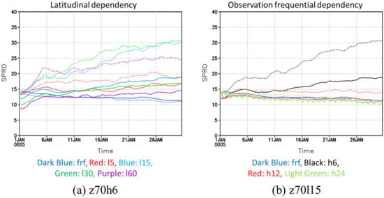
Figure A2.
Ensemble spreads (SPRD) of zonal (solid lines) and meridional (dotted lines) winds averaged at 70 km calculated by Equation (A1) from 1 January 2005. (a) Latitudinal dependency in case of assimilating data at the same time interval of 6 h. (b) Observation frequencial dependency in case of assimilating data at the same latitudinal range of 15° S–15° N. The ensemble spreads of Frf (free run forecast) are also shown in each panel.
References
- Sánchez-Lavega, A.; Lebonnois, S.; Imamura, T.; Read, P.L.; Luz, D. The Atmospheric Dynamics of Venus. Space Sci. Rev. 2017, 212, 1541–1616. [Google Scholar] [CrossRef]
- Read, P.L.; Lebonnois, S. Superrotation on Venus, on Titan, and Elsewhere. Ann. Rev. Earth Planet. Sci. 2018, 46, 175–202. [Google Scholar] [CrossRef]
- Belton, M.J.S.; Smith, G.R.; Schubert, G.; Del Genio, A.D. Cloud patterns, waves and convection in the Venus atmosphere. J. Atmos. Sci. 1976, 33, 1394–1417. [Google Scholar] [CrossRef]
- Del Genio, A.D.; Rossow, W.B. Planetary-scale waves and the cyclic nature of cloud top dynamics on Venus. J. Atmos. Sci. 1990, 47, 293–318. [Google Scholar] [CrossRef]
- Kouyama, T.; Imamura, T.; Nakamura, M.; Satoh, T.; Futaana, Y. Horizontal structure of planetary-scale waves at the cloud top of Venus deduced from Galileo SSI images with an improved cloud-tracking technique. Planet. Space Sci. 2012, 60, 207–216. [Google Scholar] [CrossRef]
- Khatuntsev, I.V.; Patsaeva, M.V.; Titov, D.V.; Ignatiev, N.I.; Turin, A.V.; Limaye, S.S.; Markiewicz, W.J.; Almeida, M.; Roatsch, T.; Moissl, R. Cloud level winds from the Venus Express Monitoring Camera imaging. Icarus 2013, 226, 140–158. [Google Scholar] [CrossRef]
- Peralta, J.; Sánchez-Lavega, A.; López-Valverde, M.A.; Luz, D.; Machado, P. Venus’s major cloud feature as an equatorially trapped wave distorted by the wind. Geophys. Res. Lett. 2015, 42, 705–711. [Google Scholar] [CrossRef]
- Hosouchi, M.; Kouyama, T.; Iwagami, N.; Ohtsuki, S.; Takagi, M. Wave signature in the Venus dayside cloud layer at 58–64 km observed by ground-based infrared spectroscopy. Icarus 2012, 220, 552–560. [Google Scholar] [CrossRef]
- Gierasch, P.J. Meridional circulation and maintenance of the Venus atmospheric rotation. J. Atmos. Sci. 1975, 32, 1038–1044. [Google Scholar] [CrossRef]
- Matsuda, Y. Dynamics of the four-day circulation in the Venus atmosphere. J. Meteorol. Soc. Jpn. 1980, 58, 443–470. [Google Scholar] [CrossRef]
- Sugimoto, N.; Takagi, M.; Matsuda, Y. Baroclinic instability in the Venus atmosphere simulated by GCM. J. Geophys. Res. 2014, 119, 1950–1968. [Google Scholar] [CrossRef]
- Ohfuchi, W.; Nakamura, H.; Yoshioka, M.K.; Enomoto, T.; Takaya, K.; Peng, X.; Yamane, S.; Nishimura, T.; Kurihara, Y.; Ninomiya, K. 10-km Mesh Meso-scale Resolving Simulations of the Global Atmosphere on the Earth Simulator, -Preliminary Outcomes of AFES (AGCM for the Earth Simulator). J. Earth Simulator 2004, 1, 8–34. [Google Scholar]
- Sugimoto, N.; Takagi, M.; Matsuda, Y. Waves in a Venus general circulation model. Geophys. Res. Lett. 2014, 41, 7461–7467. [Google Scholar] [CrossRef]
- Sugimoto, N.; Takagi, M.; Matsuda, Y. Fully developed super-rotation driven by the mean meridional circulation in a Venus GCM. Geophys. Res. Lett. 2019, 46, 1776–1784. [Google Scholar] [CrossRef]
- Ando, H.; Sugimoto, N.; Takagi, M.; Kashimura, H.; Imamura, T.; Matsuda, Y. The puzzling Venusian polar atmospheric structure reproduced by a general circulation model. Nat. Commun. 2016, 7, 10398. [Google Scholar] [CrossRef] [PubMed]
- Takagi, M.; Sugimoto, N.; Ando, H.; Matsuda, Y. Three dimensional structures of thermal tides simulated by a Venus GCM. J. Geophys. Res. Planets 2018, 123, 335–352. [Google Scholar] [CrossRef]
- Ando, H.; Takagi, M.; Fukuhara, T.; Imamura, T.; Sugimoto, N.; Sagawa, H.; Noguchi, K.; Tellmann, S.; Pätzold, M.; Häusler, B.; et al. Local time dependence of the thermal structure in the Venusian equatorial upper atmosphere: Comparison of Akatsuki radio occultation measurements and GCM results. J. Geophys. Res. Planets 2018, 123, 2970–2980. [Google Scholar] [CrossRef]
- Kashimura, H.; Sugimoto, N.; Takagi, M.; Matsuda, Y.; Ohfuchi, W.; Enomoto, T.; Nakajima, K.; Ishiwatari, M.; Sato, T.M.; Hashimoto, G.L.; et al. Planetary-scale streak structure reproduced in a Venus atmospheric simulation. Nat. Commun. 2019, 10, 23. [Google Scholar] [CrossRef]
- Yamamoto, M.; Takahashi, M. Venusian middle-atmospheric dynamics in the presence of a strong planetary-scale 5.5-day wave. Icarus 2012, 217, 702–713. [Google Scholar] [CrossRef]
- Crisp, D.; McMuldroch, S.; Stephens, S.K.; Sinton, W.M.; Ragent, B.; Hodapp, K.W.; Probst, R.G.; Doyle, L.R.; Allen, D.A.; Elias, J. Ground-Based Near-Infrared Imaging Observations of Venus During the Galileo Encounter. Science 1991, 253, 1538–1541. [Google Scholar] [CrossRef]
- Kalnay, E.; Kanamitsu, M.; Kistler, R.; Collins, W.; Deaven, D.; Gandin, L.; Iredell, M.; Saha, S.; White, G.; Woollen, J.; et al. The NCEP/NCAR 40-Year Reanalysis Project. Bull. Am. Meteorol. Soc. 1996, 77, 437–471. [Google Scholar] [CrossRef]
- Sugimoto, N.; Yamazaki, A.; Kouyama, T.; Kashimura, H.; Enomoto, T.; Takagi, M. Development of an ensemble Kalman filter data assimilation system for the Venusian atmosphere. Sci. Rep. 2017, 7, 9321. [Google Scholar] [CrossRef] [PubMed]
- Sugimoto, N.; Kouyama, T.; Takagi, M. Impact of data assimilation on thermal tides in the case of Venus Express wind observation. Geophys. Res. Lett. 2019, 46, 4573–4580. [Google Scholar] [CrossRef]
- Sugimoto, N.; Abe, M.; Kikuchi, Y.; Hosono, A.; Ando, H.; Takagi, M.; Garate-Lopez, I.; Lebonnois, S.; Ao, C. Observing system simulation experiment for radio occultation measurements of the Venus atmosphere among small satellites. J. Jpn. Soc. Civ. Eng. Ser. A2 (Appl. Mech.) 2019, 75, 477–486. [Google Scholar] [CrossRef]
- Tomasko, M.G.; Doose, L.R.; Smith, P.H.; Odell, A.P. Measurements of the flux of sunlight in the atmosphere of Venus. J. Geophys. Res. 1980, 85, 8167–8186. [Google Scholar] [CrossRef]
- Crisp, D. Radiative forcing of the Venus mesosphere: I. solar fluxes and heating rates. Icarus 1986, 67, 484–514. [Google Scholar] [CrossRef]
- Miyoshi, T.; Yamane, S. Local ensemble transform Kalman filtering with an AGCM at a T159/L48 resolution. Mon. Weather Rev. 2007, 135, 3841–3861. [Google Scholar] [CrossRef]
- Kouyama, T.; Imamura, T.; Nakamura, M.; Satoh, T.; Futaana, Y. Long-term variation in the cloud-tracked zonal velocities at the cloud top of Venus deduced from Venus Express VMC images. J. Geophys. Res. 2013, 118, 37–46. [Google Scholar] [CrossRef]
Publisher’s Note: MDPI stays neutral with regard to jurisdictional claims in published maps and institutional affiliations. |
© 2020 by the authors. Licensee MDPI, Basel, Switzerland. This article is an open access article distributed under the terms and conditions of the Creative Commons Attribution (CC BY) license (http://creativecommons.org/licenses/by/4.0/).