Winds in the Lower Cloud Level on the Nightside of Venus from VIRTIS-M (Venus Express) 1.74 μm Images

Abstract

The horizontal wind velocity vectors at the lower cloud layer were retrieved by tracking the displacement of cloud features using the 1.74 µm images of the full Visible and InfraRed Thermal Imaging Spectrometer (VIRTIS-M) dataset. This layer was found to be in a superrotation mode with a westward mean speed of 60–63 m s⁻¹ in the latitude range of 0–60° S, with a 1–5 m s⁻¹ westward deceleration across the nightside. Meridional motion is significantly weaker, at 0–2 m s⁻¹; it is equatorward at latitudes higher than 20° S, and changes its direction to poleward in the equatorial region with a simultaneous increase of wind speed. It was assumed that higher levels of the atmosphere are traced in the equatorial region and a fragment of the poleward branch of the direct lower cloud Hadley cell is observed. The fragment of the equatorward branch reveals itself in the middle latitudes. A diurnal variation of the meridional wind speed was found, as east of 21 h local time, the direction changes from equatorward to poleward in latitudes lower than 20° S. Significant correlation with surface topography was not found, except for a slight decrease of zonal wind speed, which was connected to the volcanic area of Imdr Regio.

1. Introduction

The thick cloud layer of Venus rotates around the planet in the westward direction with a peak velocity 60 times higher than that of the planet itself at approximately 100 m s⁻¹ for the altitudes of 65–70 km (upper cloud level) above the surface [1,2]; this is a phenomenon known as retrograde superrotation. In the altitude range from the surface up to 90 km, the atmospheric motion is predominantly zonal. The velocity decreases for altitude levels farther from the upper cloud level and for latitudes closer to the poles [3].

Thermal emissions from the hot lower atmosphere and surface are observed on the nightside in the near-infrared range in spectral “windows” between CO₂ bands. The lower clouds have nonhomogeneous distribution of the cloud opacity, which leads to a complex morphology of small-scale features of various observed contrasts [4]. By tracking the displacement of these cloud features with time, one can derive horizontal wind speed at the altitude of remote sensing [5].

In the spectral window of 1.74 μm on the nightside, the thermal radiance comes from the lower clouds and from beneath the main cloud level. The effective level of emissions was estimated at the altitudes of 44–48 km [5], which we will use in this paper. Thus, motion of the observed cloud features is associated with the atmosphere dynamics at these altitudes.

Before the Venus Express mission, the lower clouds of Venus were studied by the infrared spectrometer NIMS (Near-Infrared Mapping Spectrometer) onboard Galileo spacecraft [6] and from Earth-based telescopes [7,8,9,10].

Results of two cloud tracking analyses of the partial dataset of VIRTIS-M (Venus Express) images, acquired in 2006–2008 [5,11] during 18 and 45 orbits, respectively, showed a consistent zonal wind speed of ~60 m s⁻¹ between 0 and 70° S. Those works also analyzed meridional wind speed values, local time (LT), latitude and time dependence of the wind velocity in the lower clouds. Improvements brought by our analysis of the full VIRTIS-M dataset will be shown in the following sections.

More recent lower cloud tracking results came from the IR2 camera onboard JAXA’s Akatsuki spacecraft in 2016 [12,13]. Although mean meridional speed values are consistent with the VIRTIS-M results, zonal speed shows a different shape of the latitudinal profile, an “equatorial jet”, with zonal wind speed values that reached ~75 m s⁻¹ near the equator.

2. Materials and Methods

The infrared channel of the Visible and InfraRed Thermal Imaging Spectrometer (VIRTIS-M) spectrometer onboard the Venus Express covered a wavelength range between 1 and 5 μm with a spectral resolution of 14 nm and obtained images of Venus from a distance range of 40,000–70,000 km with a pixel size of 10–40 km [14]. Images were taken on the approach trajectory, when the spacecraft was moving along the high elliptical orbit towards the pericenter (located above the Northern Pole) [15]. Thus, the field of view of VIRTIS primarily captured Southern Hemisphere.

In this work, we analyzed the entire VIRTIS-M dataset, from which 195 orbits were found to be suitable (see details on analysis methods further) and from which 44,480 horizontal velocity vectors were extracted in turn (

Table 1. Number of retrieved vectors from Visible and InfraRed Thermal Imaging Spectrometer (VIRTIS-M) data depending on observation periods. Data are artificially grouped into four datasets, with approximately 2-month long intervals between them.

Dataset	Begin/End	Orbit Numbers	Orbits	Vectors
I	28 May 2006/5 October 2006	0038–0167	29	2605
II	4 December 2006/6 June 2007	0228–0411	97	23,904
III	18 July 2007/24 January 2008	0454–0644	44	12,774
IV	9 April 2008/27 October 2008	0720–0921	25	6007
All	28 May 2006/27 October 2008	0038–0921	195	44,480

). The number of analyzed orbits amounts to about 4 times the number used in previous research [11]. It allowed us to decrease the errors of the mean speed values, to provide more coverage in the equatorial latitudes and more spacious longitudinal coverage. The database of retrieved vectors can be found in the Supplementary Materials.

VIRTIS-M 1.74 μm data cover mostly (99.8%) Southern Hemisphere. Figure 1 shows how the retrieved velocity vectors are distributed across the nightside. Cloud features are most pronounced between 10 and 40° S, and as a result, this latitude range contains more than a half—51.2% of all vectors. Vectors are distributed almost symmetrically related to the midnight meridian: 45.9% are located before, 54.1%—after 0 h local time (LT). The number of retrieved vectors decreases towards both terminators.

Figure 2 shows distribution of retrieved velocity vectors in the longitude-latitude coordinates. Longitudes between 50–150° only contain 5.8% of all data. In the Southern Hemisphere, this longitude range includes Aphrodite Terra, a massive geological formation that was previously suggested to influence the atmosphere at the cloud top level on the dayside [16,17,18]. Our research took a step to investigate a possible influence of Venus topography on dynamics in the lower clouds. Unfortunately, data in the aforementioned longitude range are scarce, however some works indicated that other topographical features may also influence the atmosphere—in the upper mesosphere [19] and at the cloud top [20].

VIRTIS-M images in the 1.74 μm channel are characterized by complex cloud morphology (Figure 3), caused by varying opacity, and the abundance of cloud features that are stretched along the zonal direction due to the superrotation. Subsequent images of the same cloud area contain stable cloud features, and tracking of their displacement allows us to retrieve velocity vectors. In this work, we used images separated by 3600–7200 s intervals.

To retrieve the velocity of the displacement of identified cloud features, we used the visual method [21,22]. For a selected pair of images, acquired with a Δt interval, coordinates of any identified detail were precise enough to calculate zonal (u) and meridional (v) components of the horizontal wind by using the following formulas:

$$u=\frac{({\lambda }_2-{\lambda }_1)(R+h)\cos ({\phi }_1)}{\mathsf{\Delta }t}$$

(1)

$$v=\frac{({\phi }_2-{\phi }_1)(R+h)}{\mathsf{\Delta }t}$$

(2)

where λ_1,2 and φ_1,2 are, respectively, longitudes and latitudes of the tracked cloud features in the first and the second images; R = 6051.8 km is the radius of Venus; h = 46 km is the assumed mean altitude of the features; Δt is the time interval between two images.

VIRTIS-M nightside images in 1.74 μm have a low contrast value. To increase contrast of the cloud features, we used 2D-wavelet filtering with the Registax software (http://www.astronomie.be/registax/) [18,23,24]. An example of this filter application is shown in Figure 4, increasing the Michelson contrast value of the image from 0.75 to 0.99. This technique is especially efficient for cloud details in middle latitudes. It allows us to increase the number of identified cloud features per image pair and provide more uniform spatial coverage through retrieved velocity vectors. In the equatorial region at 0–40° S latitude, cloud details are small and have high contrast, and therefore can be easily identified (markers 1–4 in Figure 4a). In middle latitudes, cloud details become low-contrast and stretched along the latitudes. Their identification improves after the 2D-wavelet filtering (markers 5, 6 in Figure 4b).

A single measurement error can be attributed to each retrieved velocity vector. It is a positioning error of the coordinates of the identified cloud details, and it is dependent on the pixel size. The errors vary from 5–10 m s⁻¹ closer to the center of the planetary disk (usually in near polar latitudes) to 30–40 m s⁻¹ near the limb (usually in near equatorial latitudes), as was estimated for the VIRTIS-M images previously [19]. Due to high errors and potential cloud feature distortions, the 5–10° area near the limb, and therefore was avoided during the analysis.

3. Results

Most of the data obtained by VIRTIS-M covers middle and high latitudes of the Southern hemisphere on the night side with the majority of the data cubes around midnight. However, we obtained a disproportionately high number of vectors at the low and middle latitudes because of finer cloud morphology, which resulted in more cloud features to track (Figure 1 and Figure 2). The 1.74 µm VIRTIS-M data, separated in four periods of observations, are described in Table 1.

When obtaining mean values for our research, a two-step approach was made every time. First, the velocity vectors were averaged on a longitude-latitude or local time-latitude grid within each orbit. Second, orbits were averaged on the same grid. Characteristics of the analyzed mean atmospheric motion will be considered in the subsections below.

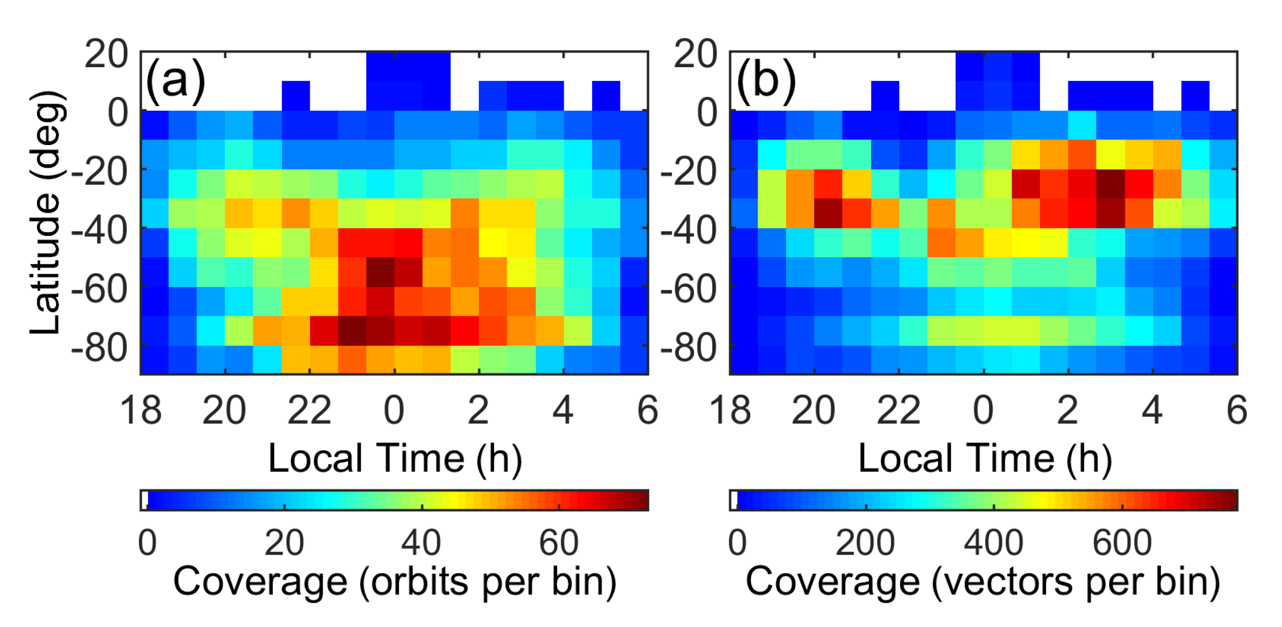
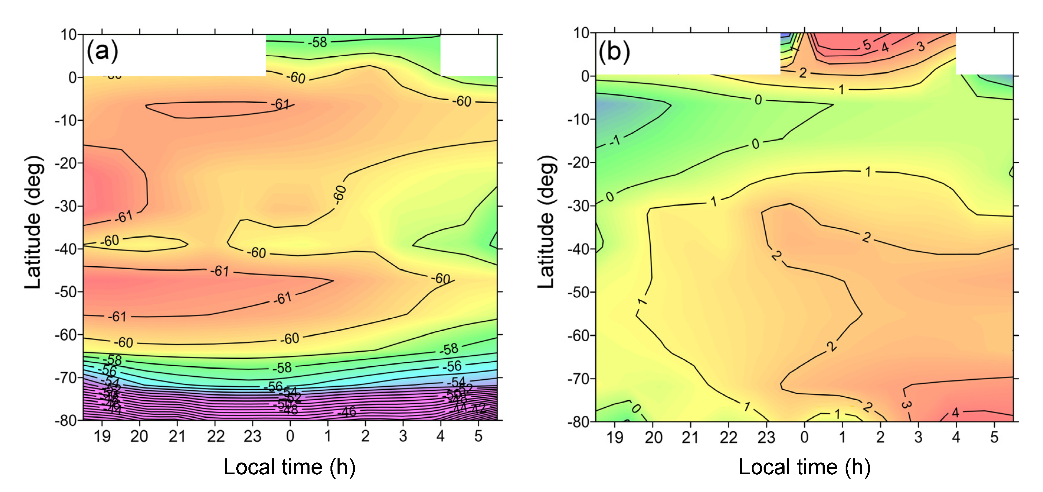
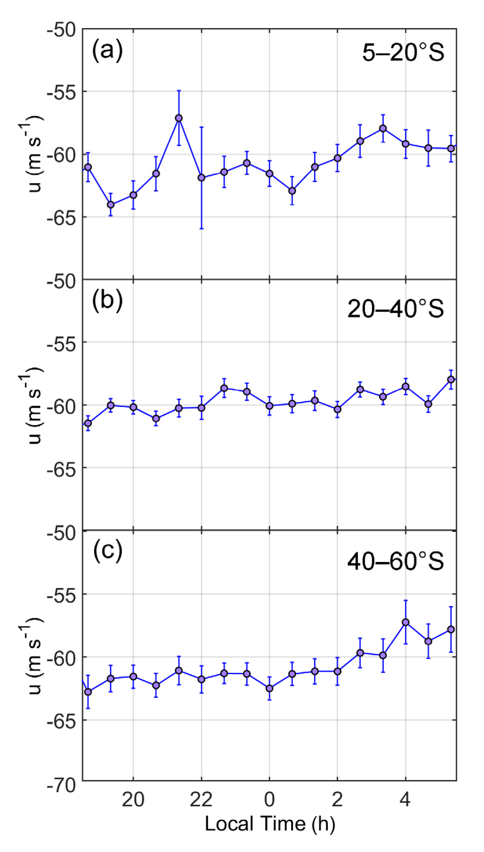
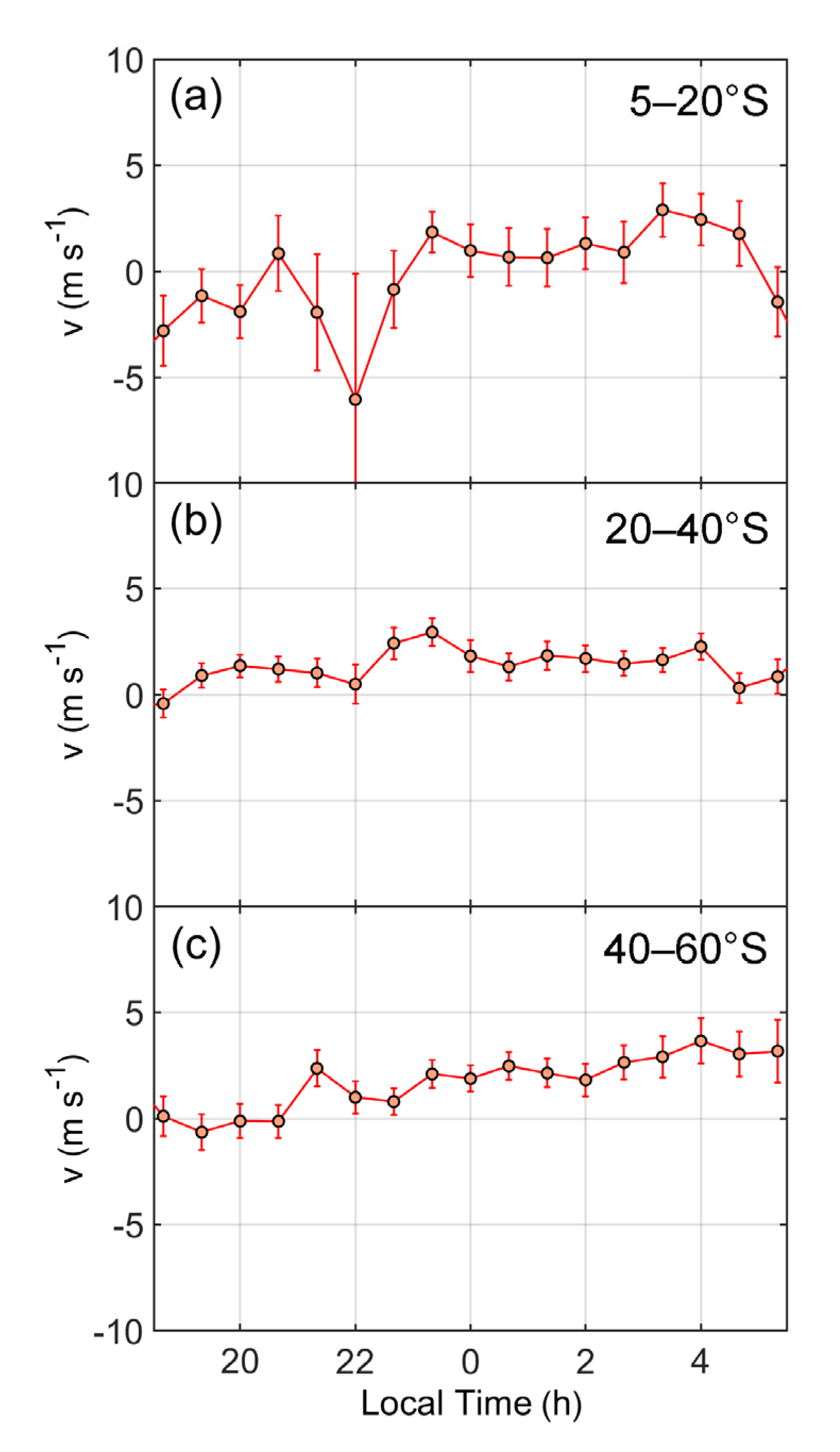
3.1. Local Time Dependence

The distributions of mean zonal and meridional wind speed in local time-latitude are given in Figure 5. The mean zonal speed in the middle latitudes reaches −60 m s⁻¹, and this result is in agreement with the superrotation mode and previous measurements [5,11]. There is a slight westward deceleration (1–5 m s⁻¹, depending on the latitude) of the zonal speed, i.e., towards the morning terminator. The nightside lowest speed (in absolute values), −58 m s⁻¹, is found at 4–5 h LT, whereas the highest u maxima of −64 m s⁻¹ are located at 19.5–21 and 23–24 h LT. Figure 6 shows local time profiles of zonal speed for cloud features found in three latitude ranges. For a confidence interval of 99% standard error, the evening-to-morning deceleration in middle latitudes is statistically significant. In the equatorial region, two zonal speed minima at 21 and 4 h LT are observed.

The meridional speed is predominantly northward (equatorward) with the values in the range 0–3 m s⁻¹. There is a statistically significant westward (towards the morning terminator) acceleration across all night side, more pronounced in the middle and high latitudes than in the low (Figure 7). After the evening terminator, at 19–20 h LT in high latitudes, the mean meridional speed changes direction and becomes southward (poleward). Additionally, the meridional speed has negative values in low latitudes between 19 and 1 h LT. This area coincides with one of the zonal speed maxima.

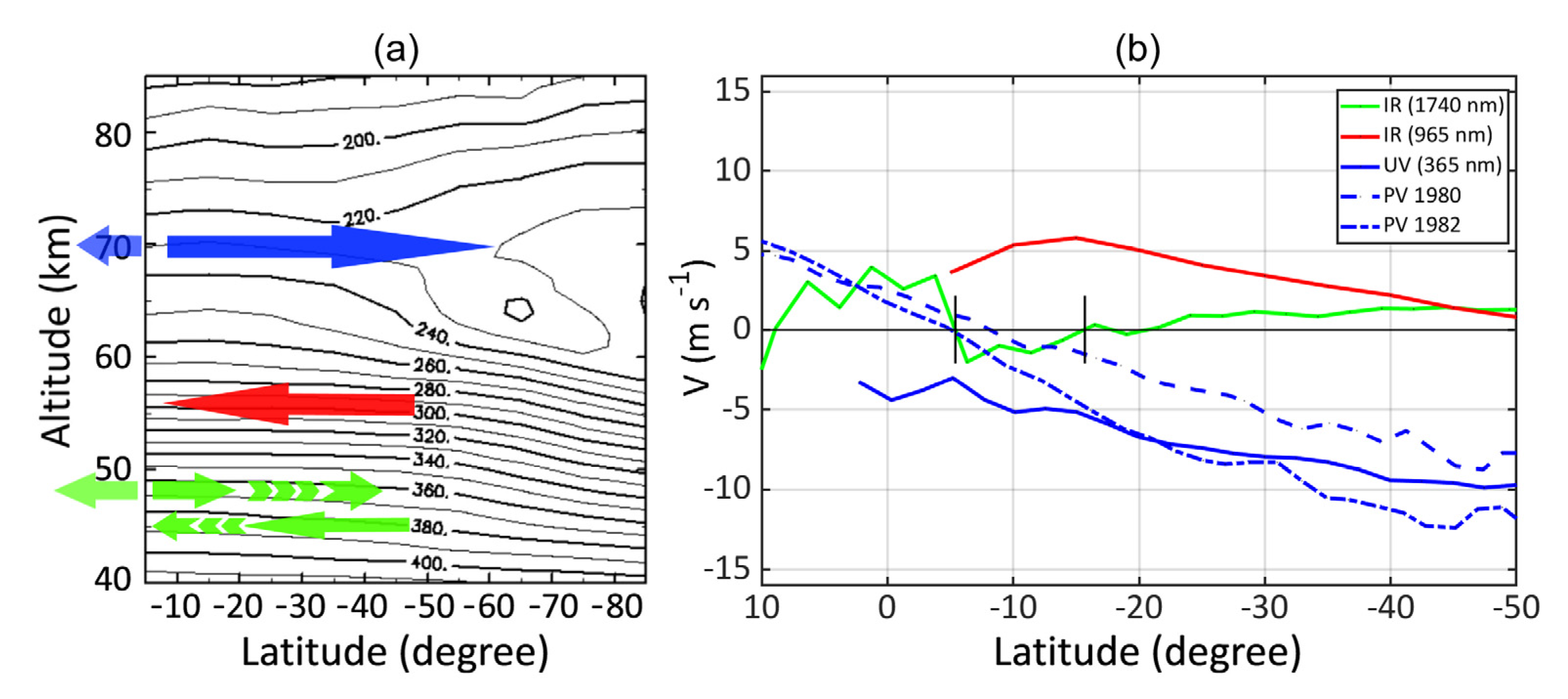
3.2. Latitudinal Dependence

Mean latitudinal profiles of the zonal and meridional wind speed are shown in Figure 8. Zonal speed stays unchanging at −60 m s⁻¹ between 20° S and 40° S. It gradually increases both northward and southward of this latitude range. To the south, between 40° S and 60° S, a jet-like increase by 2–4 m s⁻¹ was revealed. Southward of 60° S mean zonal speed decreases to zero at the South Pole.

In most of the Southern Hemisphere, mean meridional speed has a positive sign, indicating that the flow is directed north, towards the equator. This is not the case, however, for latitudes north of 15–20° S, as the meridional wind likely changes its sign to negative and horizontal flow changes to south-poleward (until about 5° S). In the equatorial region, the sign of the meridional wind changes abruptly to be positive, and up to 10° N, the horizontal flow reverts to North-poleward.

We found that the sign change of the meridional wind (from positive to negative) at 20° S coincides with the increase of the zonal speed (2–5 m s⁻¹). From the fact that we detect two flows moving towards each other, we concluded that we could observe levels at different altitudes north and south of 20° S. Despite sparse data, these variations are significant enough to be contained within a 99% confidence interval.

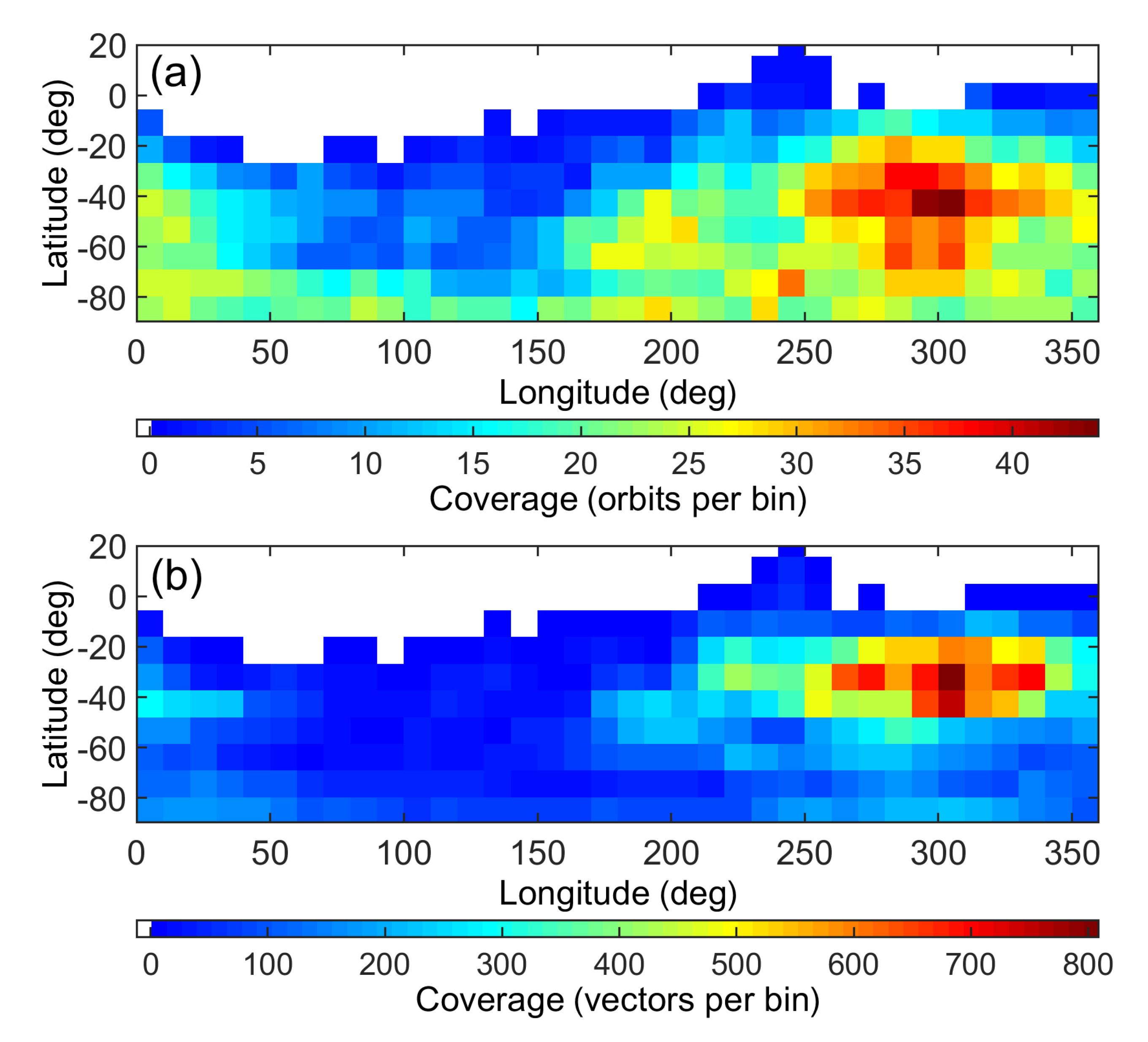
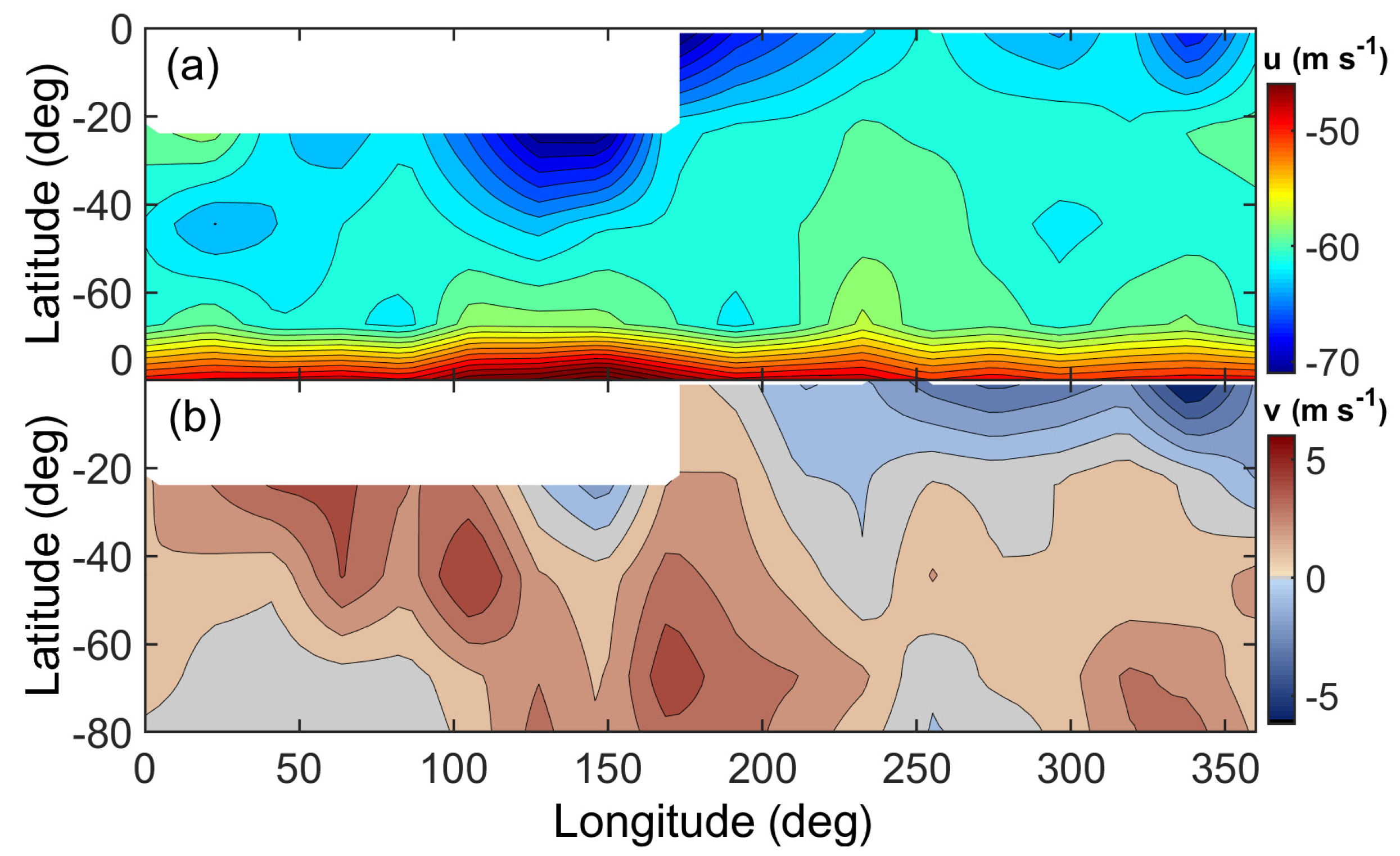
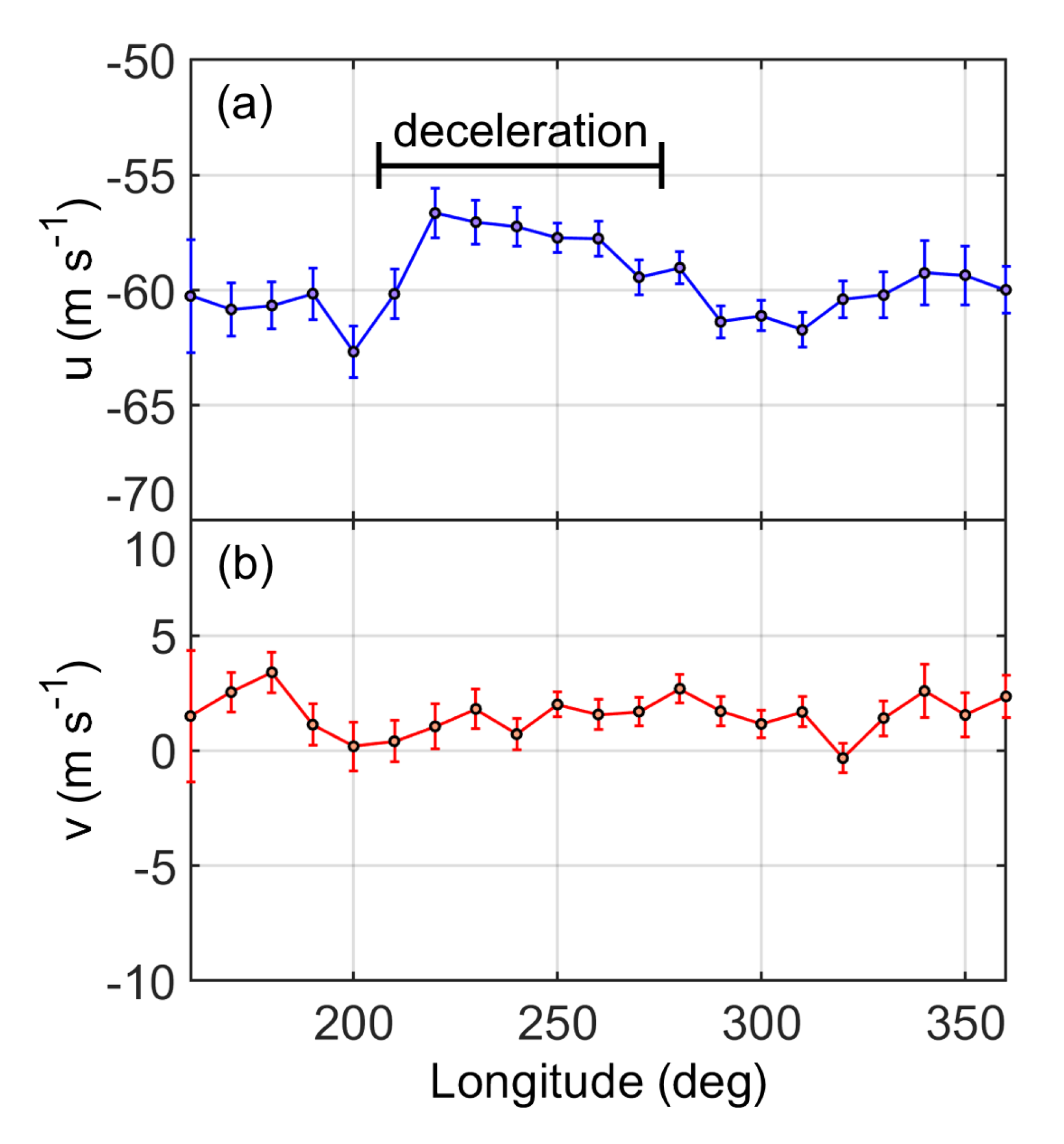
3.3. Longitudinal Dependence

Recent works have shown how Venus topography can influence atmospheric motion on different levels, at the cloud top [16,17,18,20,25] and at 90–110 km [19]. To explain observed variations, aforementioned research suggested that stationary gravity waves emerge near the surface caused by the large highland structures, terrae and regii. Topography-induced influence on the lower cloud motion was not investigated until results of the IR2 camera onboard Akatsuki showed no influence of topography, coupled with the fact that they longitude variations cannot be separated from the local time effects [13].

For VIRTIS-M data uncoupling, the longitudinal variations from the local time variations poses the same challenge. Mean wind speed distribution (Figure 9) shows variations across the Southern Hemisphere.

Strong acceleration up to −70 m s⁻¹ of the zonal wind above the plains south of Aphrodite Terra is the most prominent feature of the zonal wind distribution; however, the data in this area consists of only 10–50 vectors per a 10° × 10° bin. The slowest mean zonal wind of up to −58 m s⁻¹ is located in the middle latitudes between 210° and 260° longitude, corresponding to the area surrounding Imdr Regio on the surface. The meridional speed in the middle latitudes is closer to zero at 220°–350° longitude, whereas at 40°–200° it can reach up to 5–6 m s⁻¹ in the equatorward direction.

Figure 10 provides a more detailed look into the behavior of zonal wind in the middle latitudes. Here we consider the changes in wind speed in the 40°–50° S longitude bin. From 180° eastward, zonal speed decelerates from 62–63 m s⁻¹ to 57 m s⁻¹ at 220°–240°, then further eastward accelerates back to 62–63 m s⁻¹ at around 300° longitude. Importantly, average local time of the vectors in the aforementioned latitude and longitude range does not change sharply (no more than 0.5 h between any of the 10° × 10° bins); therefore, we rule out local time bias related to variations described in Section 3.1. Meridional wind speed does not manifest any significant change in this latitude bin.

4. Discussion

The results of our research expand on the previous partial analysis of VIRTIS-M data. Main wind speed values correspond with [5,11] within the standard error limits. A similar east-to-west increase of the meridional speed was reported, as well as the acceleration of the zonal speed in middle latitudes. However, the expansion of analyzed data allowed us to take a more detailed look at the lower cloud motion, discerning local time, latitude and longitude-dependent trends that previously were not detected. Comparison with NIMS and ground-based observations [6,7,8,9,10] also shows agreement of the mean values within their error limits.

The meridional circulation is organized as Hadley cells. A theory suggests the existence of several direct and backward cells [2]; however, experimentally only one direct cell was confirmed, in the upper clouds. General circulation models (GCM) have shown that several meridional circulation cells can exist in the lower clouds [26]. Detailed observations from UV VMC, Pioneer Venus and ground-based observations showed the South pole directed branch at the upper boundary of clouds (68–72 km), and the backward branch directed to the equator from IR VMC near the upper boundary of middle clouds [18,27,28].

As was discussed (in Section 3.2), the fact that we see two flows moving towards each other northward and southward from 20° S, signifies that we observe levels at different altitudes in the clouds. Additional insight can be achieved by analyzing the change in zonal wind speed when the meridional speed changes direction. Based on the latitudinal profile (Figure 8a) we selected two neighboring latitude ranges, where the mean meridional speed is equatorward: 20° S–40° S and poleward: 3° S–20° S. We then calculated the mean zonal speed for both ranges, which turned out to be −60.3 and −61.8 m s⁻¹, respectively, with the standard error of each value not exceeding 0.9 m s⁻¹. Taking into account that the estimated vertical shear in the lower clouds is <1 m s⁻¹ km⁻¹ [5], we suggest that the layer in the equatorial region is located about 2 km higher (48–50 km) than the layer with the positive meridional speed (44–46 km). The higher level has a negative meridional speed and horizontal flow there moves towards the South Pole, whereas in the latitudes of 20° S–40° S, at the lower level, the meridional speed is positive and the horizontal flow moves towards the equator. We assume that we observed two fragments of the lower cloud direct Hadley cell: the South pole directed branch is located at 48–50 km, and the equatorward return branch is at 44–46 km. Thus, these two fragments can be considered as the fragments of the second direct Hadley cell in the lower clouds observed at 1.74 µm. This proposition is also supported by the existence of the mid-latitude jet at 40–60° S (Figure 8a), which is most likely connected to the lower cloud direct Hadley cell.

We compared our results with previous cloud tracking in other wavelengths on the dayside from UV (VMC/VEX [22] and two Pioneer Venus profiles for two different years of observation [29]) and IR (VMC/VEX [18]) (Figure 11). Blue arrows in Figure 11a show direction of the meridional flow in the Southern (South-pole direction) and Northern (North-pole direction) Hemispheres on the upper boundary of clouds in the poleward branch of the upper clouds Hadley cell (at 70 km). The backward flow to the equator is found at around 54–58 km in middle clouds and is shown by a red arrow. Result obtained in 1.74 µm is shown by green color and consists of 3 arrows: (1) an equatorward flow south of 20° S, where the direction coincides with the red arrow; (2) a South-pole directed flow from 20° S to the equator, where the direction coincides with the blue arrow in the Southern Hemisphere; (3) a North-pole directed flow from the equator to 10° N, where the direction coincides with the blue arrow in the Northern Hemisphere, e.g., with the direction of the zonal wind on the upper boundary of clouds in Northern Hemisphere. Thus, green arrows indicate fragments of the lower-cloud direct Hadley cell, and a symmetrical lower cloud Hadley cell in the Northern Hemisphere. From the equator and up to 10° N (VIRTIS data on dynamics for higher northern latitudes are not available) the meridional wind changes its sign to positive; the horizontal flow changes its direction towards the North Pole. At these latitudes, the horizontal flow toward the North Pole is likely to correspond to the Northern hemisphere branch of the direct Hadley cell.

Observed deceleration of the zonal speed from evening to morning terminator is the most notable feature of the local time-dependent variations. A similar deceleration has been suggested for the middle clouds based on near-IR cloud tracking [18], although it was less pronounced than in our case at only up to 2 m s⁻¹, close to the error margins.

Emergence of the mid-latitude jet observed at the cloud top can be connected to a Hadley circulation cell [31]. In the lower clouds the jet found between 40° S and 60° S can as well be driven by Hadley circulation. This can also indirectly indicate that we observe fragments of a direct Hadley cell. Therefore, features described above repeat those of the upper cloud cell.

Discovered longitudinal variations are in many instances comparable to the diurnal variations (up to ±5 m s⁻¹). Moreover, searching for the influence of topography is challenging because VIRTIS nadir data do not cover any prominent highlands, such as Aphrodite Terra, instead covering several smaller ones, the tallest of which is Lada Terra (tallest areas are up to ~3 km peak altitude, located at 65–75° S/320–30° E). The notable deceleration of zonal speed, roughly in the coordinates of Imdr Regio, is a volcanic area with young lava flows and excess heat radiation [32], which as shown in Section 3.3, is stronger than any possible local time bias; however, other highlands such as Lada Terra (center at 60° S/20°E), Themis Regio (center at 40° S/280° E) and Alpha Regio (center at 22° S/5° E) do not show any coherent signs of influence on the circulation.

We can compare our results to the general circulation models. The AFES-Venus model [33] produced the same deceleration of the zonal wind from evening to morning terminator at the altitude of 50 km, as in our results (Figure 5). The local time dependency for the meridional speed also shows similarities, as the poleward motion is found before midnight, and equatorward—after midnight. Jet-like increases of zonal speed at the lower cloud level near equator and in middle latitudes has been shown by the T63 GCM [34]. Longitudinal variations have also been simulated by the GCM at ~54 km [35]. Although the general behavior of wind velocity does not coincide with our results (Figure 9), model meridional speed was found to show more variability compared to the zonal speed.

5. Conclusions

In this work, the full set of VIRTIS data was processed and analyzed. It allowed us to study four times more data than in the previous works and to obtain some new findings.

An experimental indication for the existence of the lower cloud direct Hadley cell was found for the first time. Although GCMs allow the existence of one or more cells in the lower atmosphere, they were not experimentally found before.

Dynamics of the Venusian atmosphere is very variable (if we compare VIRTIS and Akatsuki measurements), and we were lucky that during VIRTIS observations, a lower cloud layer was arranged in such a way that in the same wavelength (1.74 µm), we could observe the levels at different altitudes in the atmosphere depending on latitude. Parallel with the change in the value of the zonal speed, we also observed the change of the sign of the meridional speed, which leads to a conclusion that there most likely are different circulation cells in the considered altitude range of the atmosphere.

It is known that in the upper cloud meridional circulation is organized as a direct Hadley cell, with the upper branch directed to the pole at the altitude of 68–70 km and the lower one directed to the equator more than 10 km below. The mid-latitude jet is considered as being connected to the Hadley cell.

Meridional flow directions of the upper cloud Hadley cell branches and the observed lower cloud cell branches show a correlation. The mid-latitude jet observed at 40–60° S in the lower clouds, most likely connected to the lower cloud cell, also resembles the jet in the upper cloud layer. Thus, by analogy with the direct Hadley cell in the upper cloud layer, we came to a conclusion that in 1.74 µm, we observe fragments of the direct Hadley cell in the lower cloud layer.

References

1. Schubert, G. General circulation and dynamical state of the Venus atmosphere. In Venus; Hunten, D., Colin, L., Donahue, T., Moroz, V.I., Eds.; University of Arizona Press: Tucson, AZ, USA, 1983; pp. 681–765. [Google Scholar]
2. Gierasch, P.J.; Goody, R.M.; Young, R.E.; Crisp, D.; Edwards, C.; Kahn, R.; Rider, D.; del Genio, A.; Greeley, R.; Hou, A.; et al. The general circulation of the Venus atmosphere: An assessment. In Venus II—Geology, Geophysics, Atmosphere, and Solar Wind Environment; Bougher, J.W., Hunten, D.M., Phillips, R.J., Eds.; University of Arizona Press: Tucson, AZ, USA, 1997; pp. 459–500. [Google Scholar]
3. Zasova, L.V.; Linkin, V.M.; Khatuntsev, I.V. Zonal wind in the middle atmosphere of Venus. Cosm. Res. 2000, 38, 54–70. [Google Scholar]
4. McGouldrick, K.; Momary, T.W.; Baines, K.H.; Grinspoon, D.H. Quantification of middle and lower cloud variability and mesoscale dynamics from Venus Express/VIRTIS observations at 1.74 μm. Icarus 2012, 217, 615–628. [Google Scholar] [CrossRef]
5. Sánchez-Lavega, A.; Hueso, R.; Piccioni, G.; Drossart, P.; Peralta, J.; Pérez-Hoyos, S.; Wilson, C.F.; Taylor, F.W.; Baines, K.H.; Luz, D.; et al. Variable winds on Venus mapped in three dimensions. Geophys. Res. Lett. 2008, 35, L13204. [Google Scholar] [CrossRef] [Green Version]
6. Carlson, R.W.; Baines, K.H.; Kamp, L.W.; Weissman, P.R.; Smythe, W.D.; Ocampo, A.C.; Johnson, T.V.; Matson, D.L.; Pollack, J.B.; Grinspoon, D. Galileo infrared imaging spectroscopy measurements at Venus. Science 1991, 253, 1541–1548. [Google Scholar] [CrossRef]
7. Crisp, D.; McMuldroch, S.; Stephens, S.K.; Sinton, W.M.; Ragent, B.; Hodapp, K.-W.; Probst, R.G.; Doyle, L.R.; Allen, D.A.; Elias, J. Ground-based near-infrared imaging observations of Venus during the Galileo encounter. Science 1991, 253, 1538–1541. [Google Scholar] [CrossRef]
8. Tavenner, T.; Young, E.F.; Bullock, M.A.; Murphy, J.; Coyote, S. Global mean cloud coverage on Venus in the near-infrared. Planet. Space Sci. 2008, 56, 1435–1443. [Google Scholar] [CrossRef]
9. Young, E.F.; Bullock, M.A.; Tavenner, T.; Coyote, S.; Murphy, J.R. Temporal variability and latitudinal jets in Venus’s zonal wind profiles. Bull. Am. Astron. Soc. 2008, 40, 513. [Google Scholar]
10. Young, E.F.; Bullock, M.A.; Limaye, S.; Bailey, K.; Tsang, C.C.C. Evidence for and against 8-day planetary waves in ground-based cloud-tracking observations of Venus’ nightside. Bull. Am. Astron. Soc. 2010, 42, 975. [Google Scholar]
11. Hueso, R.; Peralta, J.; Sánchez-Lavega, A. Assessing the long-term variability of Venus winds at cloud level from VIRTIS–Venus Express. Icarus 2012, 217, 575–598. [Google Scholar] [CrossRef]
12. Horinouchi, T.; Murakami, S.; Satoh, T.; Peralta, J.; Ogohara, K.; Kouyama, T.; Imamura, T.; Kashimura, H.; Limaye, S.S.; McGouldrick, K.; et al. Equatorial jet in the lower to middle cloud layer of Venus revealed by Akatsuki. Nat. Geosci. 2017, 10, 646–651. [Google Scholar] [CrossRef]
13. Peralta, J.; Muto, K.; Hueso, R.; Horinouchi, T.; Sánchez-Lavega, A.; Murakami, S.; Machado, P.; Young, E.F.; Lee, Y.J.; Kouyama, T.; et al. Nightside Winds at the Lower Clouds of Venus with Akatsuki/IR2: Longitudinal, Local Time, and Decadal Variations from Comparison with Previous Measurements. ApJS 2018, 239, 29–239. [Google Scholar] [CrossRef] [Green Version]
14. Piccioni, G.; Drossart, P.; Suetta, E.; Cosi, M.; Amannito, E.; Barbis, A.; Berlin, R.; Bocaccini, A.; Bonello, G.; Bouyé, M.; et al. VIRTIS: The Visible and Infrared Thermal Imaging Spectrometer. ESA Spec. Publ. 2007, SP 1295, 1–27. [Google Scholar]
15. Svedhem, H.; Titov, D.V.; Taylor, F.W.; Witasse, O. The Venus Express mission. J. Geophys. Res. 2009, 114, E00B33. [Google Scholar] [CrossRef] [Green Version]
16. Bertaux, J.-L.; Khatuntsev, I.V.; Hauchecorne, A.; Markiewicz, W.J.; Marcq, E.; Lebonnois, S.; Patsaeva, M.; Turin, A.; Fedorova, A. Influence of Venus topography on the zonal wind and UV albedo at cloud top level: The role of stationary gravity waves. J. Geophys. Res. Planets 2016, 121, 1087–1101. [Google Scholar] [CrossRef] [Green Version]
17. Fukuhara, T.; Futaguchi, M.; Hashimoto, G.L.; Horinouchi, T.; Imamura, T.; Iwagaimi, N.; Kouyama, T.; Murakami, S.; Nakamura, M.; Ogohara, K.; et al. Large stationary gravity wave in the atmosphere of Venus. Nat. Geosci. 2017, 10, 85–88. [Google Scholar] [CrossRef]
18. Khatuntsev, I.V.; Patsaeva, M.V.; Titov, D.V.; Ignatiev, N.I.; Turin, A.V.; Fedorova, A.A.; Markiewicz, W.J. Winds in the middle cloud deck from the near-IR imaging by the Venus Monitoring Camera onboard Venus Express. J. Geophys. Res. Planets 2017, 122, 2312–2327. [Google Scholar] [CrossRef] [Green Version]
19. Gorinov, D.A.; Khatuntsev, I.V.; Zasova, L.V.; Turin, A.V.; Piccioni, G. Circulation of Venusian atmosphere at 90–110 km based on apparent motions of the O2 1.27 μm nightglow from VIRTIS-M (Venus Express) data. Geophys. Res. Lett. 2018, 45, 2554–2562. [Google Scholar] [CrossRef]
20. Fukuya, K.; Imamura, T.; Taguchi, M.; Fukuhara, T.; Kouyama, T. Faint thermal features at the Venusian cloud top found by averaging multiple infrared images taken by Akatsuki. In Proceedings of the EPSC-DPS Joint Meeting, Geneva, Switzerland, 15–20 September 2019. [Google Scholar]
21. Moissl, R.; Khatuntsev, I.; Limaye, S.S.; Titov, D.V.; Markiewicz, W.J.; Ignatiev, N.I.; Roatsch, T.; Matz, K.-D.; Jaumann, R.; Almeida, M.; et al. Cloud top winds from tracking UV features in Venus Monitoring Camera images. J. Geophys. Res. 2009, 114. [Google Scholar] [CrossRef] [Green Version]
22. Khatuntsev, I.V.; Patsaeva, M.V.; Titov, D.V.; Ignatiev, N.I.; Turin, A.V.; Limaye, S.S.; Markiewicz, W.J.; Almeida, M.; Roatsch, T.; Moissl, R. Cloud level winds from the Venus Express Monitoring Camera imaging. Icarus 2013, 226, 140–158. [Google Scholar] [CrossRef]
23. Lim, A.; Jaenisch, H.; Handley, J.; Filipovic, M.; White, G.; Hons, A.; Berrevoets, C.; Deragopian, G.; Payne, J.; Schneider, M.; et al. Image Resolution and Performance Analysis of Webcams for Ground-Based Astronomy. Available online: https://spie.org/publications/conference-proceedings/browse-by-year/browse-list-of-proceedings-for-a-year?start_year=2004&end_year=2004 (accessed on 30 January 2021).
24. Berrevoets, C.; DeClerq, B.; George, T.; Makolkin, D.; Maxson, P.; Pilz, B.; Presnyakov, P.; Eric, R.; Weiller, S. RegiStax: Alignment, Stacking and Processing of Images. Available online: https://ui.adsabs.harvard.edu/abs/2012ascl.soft06001B/abstract (accessed on 30 January 2021).
25. Patsaeva, M.V.; Khatuntsev, I.V.; Zasova, L.V.; Hauchecorne, A.; Titov, D.V.; Bertaux, J.-L. Solar-Related Variations of the Cloud Top Circulation Above Aphrodite Terra From VMC/Venus Express Wind Fields. J. Geophys. Res. 2019, 124, 1864–1879. [Google Scholar] [CrossRef]
26. Sugimoto, N.; Takagi, M.; Masuda, Y. Fully developed superrotation driven by the mean meridional circulation in a Venus GCM. Geophys. Res. Lett. 2019, 46, 1776–1784. [Google Scholar] [CrossRef]
27. Machado, P.; Widemann, T.; Peralta, J.; Gonçalves, R.; Donati, J.-F.; Luz, D. Venus cloud-tracked and doppler velocimetry winds from CFHT/ESPaDOnS and Venus Express/VIRTIS in April 2014. Icarus 2017, 285, 8–26. [Google Scholar] [CrossRef]
28. Gonçalves, R.; Machado, P.; Widemann, T.; Peralta, J.; Watanabe, S.; Yamazaki, A.; Satoh, T.; Takagi, M.; Ogohara, K.; Lee, Y.-J.; et al. Venus’ cloud top wind study: Coordinated Akatsuki/UVI with cloud tracking and TNG/HARPS-N with Doppler velocimetry observations. Icarus 2020, 335, 113418. [Google Scholar] [CrossRef]
29. Limaye, S.S. Venus atmospheric circulation: Known and unknown. J. Geophys. Res. 2007, 112, JE002814. [Google Scholar] [CrossRef] [Green Version]
30. Ando, H.; Imamura, T.; Tellmann, S.; Pätzold, M.; Häusler, B.; Sugimoto, N.; Takagi, M.; Sagawa, H.; Limaye, S.; Matsuda, Y.; et al. Thermal structure of the Venusian atmosphere from the sub-cloud region to the mesosphere as observed by radio occultation. Sci. Rep. 2020, 10, 1–7. [Google Scholar] [CrossRef] [PubMed] [Green Version]
31. Yamamoto, M.; Takahashi, M. General circulation driven by baroclinic forcing due to cloud layer heating: Significance of planetary rotation and polar eddy heat transport. J. Geophys. Res. Planets 2016, 121, 558–573. [Google Scholar] [CrossRef] [Green Version]
32. D’Incecco, P.; López, I.; Komatsu, G.; Ori, G.G.; Aittola, M. Local stratigraphic relations at Sandel crater, Venus: Possible evidence for recent volcano-tectonic activity in Imdr Regio. Earth Planet. Sci. Lett. 2020, 546, 116410. [Google Scholar] [CrossRef]
33. Takagi, M.; Sugimoto, N.; Ando, H.; Matsuda, Y. Three-dimensional structures of thermal tides simulated by a Venus GCM. J. Geophys. Res. Planets 2018, 123, 335–352. [Google Scholar] [CrossRef]
34. Yamamoto, M.; Ikeda, K.; Takahashi, M. Atmospheric response to high-resolution topographical and radiative forcings in a general circulation model of Venus: Time-mean structures of waves and variances. Icarus 2021, 355, 114154. [Google Scholar] [CrossRef]
35. Yamamoto, M.; Ikeda, K.; Takahashi, M.; Horinouchi, T. Solar-locked and geographical atmospheric structures inferred from a Venus, general circulation model with radiative transfer. Icarus 2019, 321, 232–250. [Google Scholar] [CrossRef]
Figure 1. Coverage of Venus nightside by velocity vectors retrieved in this work. This distribution uses 40 min LT × 10° latitude bins. (a): number of orbits (per bin) that were eligible for velocity retrieval. (b): number of vectors (per bin) retrieved in total.
Atmosphere 12 00186 g001
Figure 2. Coverage of Venus nightside in longitude—latitude coordinates by velocity vectors retrieved in this work. This distribution uses 10° longitude × 10° latitude bins. (a): number of orbits (per bin) that were eligible for velocity retrieval. (b): number of vectors (per bin) retrieved in total.
Atmosphere 12 00186 g002
Figure 3. Examples of images by VIRTIS in 1.74 μm, taken from a slant distance of 60,000–65,000 km: (a) orbit 71, data cube 01, 30 June 2006 15:06; (b) orbit 367, data cube 02, 22 August 2007 21:44; (c) orbit 569, data cube 05, 10 November 2007 16:11; (d) orbit 812, data cube 04, 10 June 2008 20:15.
Atmosphere 12 00186 g003
Figure 4. Example of applying a 2D-wavelet filter to a VIRTIS-M image (data cube 569_13). Arrows indicate examples of identified cloud details used in the wind velocity retrieval. (a): original image, (b): same image after filter application.
Atmosphere 12 00186 g004
Figure 5. Mean zonal (a) and meridional (b) speed in the lower clouds as a function of local time and latitude. Areas where no velocity vectors were available are left blank.
Atmosphere 12 00186 g005
Figure 6. Local time profiles of the zonal wind speed constrained in latitude bins of 5–20° S (a), 20–40° S (b) and 40–60° S (c). Error bars show standard error for a 99% confidence interval.
Atmosphere 12 00186 g006
Figure 7. Local time profile of the meridional wind speed constrained in latitude bins of 5–20° S (a), 20–40° S (b) and 40–60° S (c). Error bars show standard error for a 99% confidence interval.
Atmosphere 12 00186 g007
Figure 8. Mean profiles of the zonal (a) and meridional (b) winds in the lower clouds of Venus on the nightside from the full VIRTIS-M dataset. The average values were calculated for 2.5° latitude bins. Error bars show standard errors for a 99% confidence interval.
Atmosphere 12 00186 g008
Figure 9. Longitudinal distribution of the zonal (a) and the meridional (b) wind velocities from VIRTIS-M data, indicated by isolines.
Atmosphere 12 00186 g009
Figure 10. Longitudinal profiles (160–360°) of the zonal (a) and the meridional (b) wind speed in the 40°–50° S latitude bin. Error bars show standard error for a 99% confidence interval.
Atmosphere 12 00186 g010
Figure 11. (a) Mean direction of the meridional wind at different altitudes (arrows) overlaid on the thermal structure of the atmosphere in latitude-altitude coordinates from combined Venus Express and Akatsuki radio occultation experiment results, averaged over both hemispheres [30]. We changed the latitude sign to negative to adopt the figure to the Southern hemisphere. Numbers at the contours indicate the temperature in Kelvin. Latitudes represent both hemispheres assuming north-south symmetry. The thermal structure is used for illustration to designate different levels in the Southern Hemisphere. Blue arrows represent UV cloud tracking results (PV and VMC/VEX), red arrow: IR cloud tracking from VMC/VEX, green arrows: 1.74 µm (1740 nm) IR cloud tracking from VIRTIS/VEX. Dashed green arrows indicate branches of Hadley cells that are not observable in the experiment. (b) Mean latitudinal profiles of the meridional wind from several experiments; line colors correspond with those in (a), line types correspond with the legend. Two vertical lines located at v = 0 axis limit the latitude range of the 1.74 µm cloud tracking profile (green line) where the meridional wind becomes south-poleward.
Atmosphere 12 00186 g011