Improved Hargreaves Model Based on Multiple Intelligent Optimization Algorithms to Estimate Reference Crop Evapotranspiration in Humid Areas of Southwest China

Abstract

Reference crop evapotranspiration (ET₀) is an important indicator for precise regulation of crop water content, irrigation forecast formulation, and regional water resources management. The Hargreaves model (HG) is currently recognized as the simplest and most effective ET₀ estimation model. To further improve the prediction accuracy of the HG model, this study is based on the data of 98 meteorological stations in southwest China (1961–2019), using artificial bee colony (ABC), differential evolution (DE) and particle swarm optimization (PSO) algorithms to calibrate the HG model globally. The standard ET₀ value was calculated by FAO-56 Penman–Monteith (PM) model. We compare the calculation accuracy of 3 calibrated HG models and 4 empirical models commonly used (Hargreaves, Priestley–Taylor, Imark–Allen and Jensen–Hais). The main outcomes demonstrated that on a daily scale, the calibrated HG models (R² range 0.74–0.98) are more accurate than 4 empirical models (R² range 0.55–0.84), and ET_0-PSO-HG has the best accuracy, followed by ET_0-ABC-HG and ET_0-DE-HG, with average R² of 0.83, 0.82 and 0.80, average RRMSE of 0.23 mm/d, 0.25 mm/d and 0.26 mm/d, average MAE of 0.52 mm/d, 0.53 mm/d and 0.57 mm/d, and average GPI of 0.17, 0.05, and 0.04, respectively; on a monthly scale, ET_0-PSO-HG also has the highest accuracy, followed by ET_0-ABC-HG and ET_0-DE-HG, with median R² of 0.96, 0.95 and 0.94, median RRMSE of 0.16 mm/d, 0.17 mm/d and 0.18 mm/d respectively, median MAE of 0.46 mm/d, 0.50 mm/d, and 0.55 mm/d, median GPI of 1.12, 0.44 and 0.34, respectively. The calibrated HG models (relative error of less than 10.31%) are also better than the four empirical models (relative error greater than 16.60%). Overall, the PSO-HG model has the most accurate ET₀ estimation on daily and monthly scales, and it can be suggested as the preferred model to predict ET₀ in humid regions in southwest China regions.

1. Introduction

Reference crop evapotranspiration (ET₀) is a major parameter for climate researches and agricultural water resources management [1]. This essential indicator is not only important to measure water balance and conversion, but also plays a significant role in the process of energy exchange between the earth and the atmosphere [2,3]. Therefore, accurate estimation of ET₀ is valuable for the estimation of agricultural water demand, irrigation forecast, the management of regional water resources and budget [4,5].

In recent years, many mathematical models can be used to estimate the ET₀, including FAO-56 Penman–Monteith (PM) [6], Imark–Allen [7], Priestley–Taylor [8], Hargreaves [9], Jensen–Haise [10] and Makkink [11]. Among them, the Penman–Monteith model is the most common one applied in the study of evapotranspiration, and there are many variations about it [12,13]. The PM model is applied to various environmental and climatic conditions without local or global correction, and the estimation result is accurate. Therefore, it is often used as the standard to verify other models [13]. The main limitation of the PM model is that it requires many meteorological elements [14]. The most ideal process, then, is to estimate ET based on as few input elements as possible without affecting the accuracy [15,16].

The radiations model has also attracted the attention of many researchers because it requires less input data and the temperature is easy to measure [17]. The famous Hargreaves (HG) model estimates ET₀ only by inputting the maximum and minimum temperature and solar radiation, so this method is considered to one of the simplest and accurate methods to estimate ET₀ [18,19,20,21]. Hence, when the data required by the PM model cannot be fully obtained, the short-term prediction of ET₀ can be done by using the HG model. Liu et al. [22] evaluated 16 methods for estimating ET₀ based on radiation models and among them, the HG model has more accurate average performance indicators in the arid, semi-arid, temperate, also in frigid and polar climates. At the same time, some scholars pointed out that the HG model needs global calibration, which is suitable for the estimation of ET₀ in long time series. Almorox et al. [23] and Feng et al. [24] found that under low humidity or strong wind conditions (u > 3 m/s) the HG model estimation result is relatively low, while the estimation result ET₀ is relatively high when the levels of humidity are high. Therefore, the HG model might need to be calibrated to accurately estimate ET₀.

In recent years, with the development of AI technology, machine learning optimization algorithms have also provided some useful information to the field. Feng et al. [25] discussed four different machine learning models: extreme learning machine (ELM), generalized regression neural network (GRNN), back-propagation neural network (BPNN) and random forest (RF) model and predict soil temperature (TS) on different depths of 2 cm, 5 cm, 10 cm and 20 cm on the Loess Plateau and the results showed that ELM, GRNN, BPNN and RF models can accurately estimate TS at different depths. Zhu et al. [26] used particle swarm optimization (PSO) to optimize the extreme value learning machine (ELM) model under the condition of limited meteorological data and proposed a hybrid model (PSO-ELM) to accurately predict daily ET₀ in the arid area of Northwest China. In the past few decades, several scholars have done a lot of work on the calibration of the HG model [27,28], however, these calibrations are specific to some locations and cannot be applied to other places with totally different climatic conditions. Moreover, the structure of the improved HG model is more complex than the original model [29,30,31]. With that being said, it is possible to shape the aims of this research as (i) calibrate the 3 empirical parameters (C, m, a) in the HG model based on artificial honeycomb (ABC), differential optimization (DE) and particle swarm (PSO) optimisation algorithms; (ii) evaluate the ET₀ estimation accuracy of 3 improved HG models and the Priestley–Taylor, Imark–Allen and Jensen–Haise models on different time scales; and (iii) propose recommended models for ET₀ estimation in Southwest China at different scales.

2. Materials and Methods

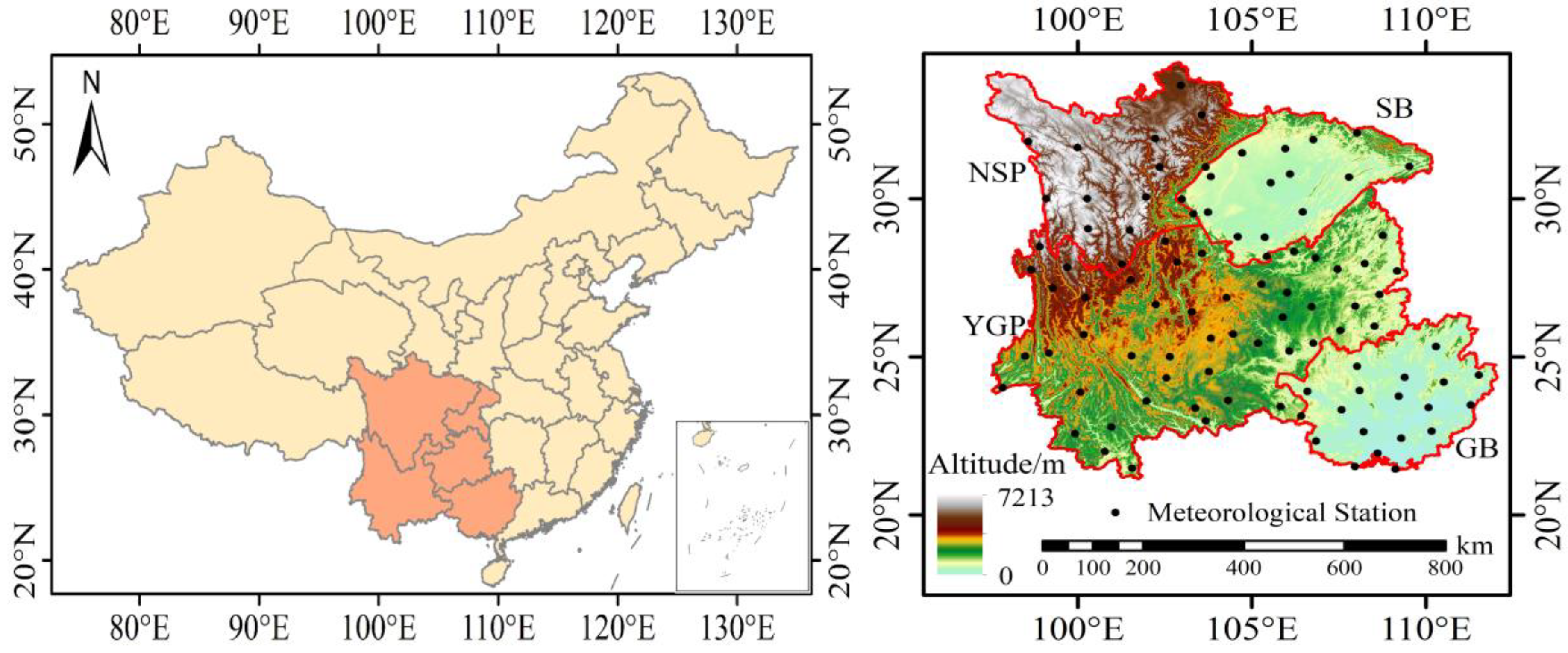
2.1. Study Area and Weather Data

The southwest region of China mainly includes the Northwest Sichuan Plateau (NSP), the Sichuan Basin (SB), the Guangxi Basin (GB) and the Yunnan–Guizhou Plateau (YGP). The SB is one of the main grain-producing areas in the country, with an area of about 260,000 km² and a population of 90 million. The famous Dujiangyan project located in the middle of the SB, with an irrigation area of about 67,000 km². The NSP is one of the five largest pastoral areas in China and the largest animal husbandry base in Sichuan, covering an area of approximately 166,000 km². The terrain of the GB is higher in the northwest and lower in the southeast, and the elevation is generally 80 to 200 m, mostly limestone, covering an area of about 70%, with obvious karst landforms. The YGP located in southwestern China and is one of the four major plateaus with a total area of about 500,000 km². This specific distribution is shown in Figure 1.

The meteorological data used in this article comes from the National Climate Centre of the China Meteorological Administration (http://data.cma.cn). The southwest region mainly includes 98 meteorological stations–more information is shown in

Table 1. Mean values of the main climate variables of meteorological stations in Southwest China from 1961 to 2019.

Zone	Station	Lat	Lon	H	Tmean	DTR	Ra	Zone	Station	Lat	Lon	H	Tmean	DTR	Ra
		(°)	(°)	(m)	°C	°C	MJ/m2 d			(°)	(°)	(m)	°C	°C	MJ/m2 d
NSP	1. Batang	30.00	99.10	2589.20	6.33	14.36	30.96	YGP	1. Napo	23.42	105.83	794.10	19.88	7.74	33.18
	2. Daocheng	29.05	100.30	3727.70	5.61	15.59	31.72		2. Anshun	26.25	105.90	1431.10	14.82	6.81	32.50
	3. Dege	31.80	98.58	3184.00	8.13	15.10	30.98		3. Bijie	27.30	105.28	1510.60	13.86	8.09	32.23
	4. Emeishan	29.52	103.33	3047.40	4.08	7.16	31.62		4. Dushan	25.83	107.55	1013.30	15.87	7.23	32.66
	5. Ganzi	31.62	100.00	3393.50	7.00	14.63	30.94		5. Guiyang	26.58	106.73	1223.80	15.85	7.52	32.45
	6. Jiulong	29.00	101.50	2987.30	10.27	14.43	31.70		6. Kaili	26.60	107.98	720.30	16.68	7.93	32.44
	7. Kangding	30.05	101.97	2615.70	8.20	9.11	31.41		7. Luodian	25.43	106.77	440.30	20.73	9.26	32.72
	8. Litang	30.00	100.27	3948.90	4.49	13.62	31.50		8. Meitan	27.77	107.47	792.20	15.81	7.26	32.16
	9. Maerkang	31.90	102.23	2664.40	10.59	16.11	30.96		9. Panxian	25.72	104.47	1800.00	15.94	9.20	32.68
	10. Muli	27.93	101.27	2426.50	13.50	12.66	32.10		10. Qianxi	27.03	106.02	1231.40	14.83	7.64	32.27
	11. Ruoergai	33.58	102.97	3439.60	2.30	14.37	30.41		11. Ronjiang	25.97	108.53	285.70	19.43	8.69	32.64
	12. Songpan	32.65	103.57	2850.70	7.54	14.38	30.71		12. Sansui	26.97	108.67	626.90	15.83	8.08	32.39
	13. Xiaojin	31.00	102.35	2369.20	13.33	13.56	31.13		13. Sinan	27.95	108.25	416.30	18.10	7.38	32.13
GB	1. Baise	23.90	106.60	173.50	23.01	9.07	33.11		14. Tongzi	28.13	106.83	972.00	15.47	7.12	31.99
	2. Beihai	21.45	109.13	12.80	23.37	6.51	33.62		15. Tongren	27.72	109.18	279.70	17.95	8.10	32.16
	3. Dongxing	21.53	107.97	22.10	23.30	6.44	33.61		16. Wangmo	25.18	106.08	566.80	20.36	9.43	32.76
	4. Duan	23.93	108.10	170.80	22.12	7.01	33.10		17. Weining	26.87	104.28	2237.50	11.78	9.29	32.40
	5. Guilin	25.32	110.30	164.40	19.76	7.33	32.71		18. Xishui	28.33	106.22	1180.20	13.84	6.71	31.96
	6. Guiping	23.40	110.08	42.50	22.42	7.00	33.18		19. Xingyi	25.43	105.18	1378.50	16.20	8.12	32.72
	7. Hechi	24.70	108.03	260.20	21.31	7.45	32.90		20. Huili	26.65	102.25	1787.30	16.06	12.22	32.41
	8. Hexian	24.42	111.53	108.80	20.85	8.27	32.94		21. Leibo	28.27	103.58	1255.80	13.52	6.44	31.94
	9. Jingxi	23.13	106.42	739.90	20.08	7.20	33.22		22. Yanyuan	27.43	101.52	2545.00	13.12	12.03	32.21
	10. Laibin	23.75	109.23	84.90	21.66	7.82	33.13		23. Yuexi	28.65	102.52	1659.50	14.43	10.59	31.87
	11. Lingshan	22.42	109.30	66.60	22.46	7.67	33.40		24. Zhaojue	28.00	102.85	2132.40	12.37	10.44	31.98
	12. Liuzhou	24.35	109.40	96.80	21.50	7.43	32.95		25. Baoshan	25.12	99.18	1652.20	16.79	11.40	32.74
	13. Longzhou	22.33	106.85	128.80	23.21	8.33	33.41		26. Chuxiong	25.03	101.55	1824.10	16.77	11.35	32.75
	14. Mengshan	24.20	110.52	145.70	20.71	7.94	32.97		27. Dali	25.70	100.18	1990.50	15.71	10.95	32.65
	15. Nanning	22.63	108.22	121.60	22.48	7.83	33.37		28. Deqin	28.48	98.92	3319.00	6.75	9.96	31.90
	16. Pingguo	23.32	107.58	108.80	22.64	8.06	33.19		29. Gongshan	27.75	98.67	1583.30	15.93	10.77	32.13
	17. Qinzhou	21.95	108.62	4.50	23.01	6.75	33.55		30. Huize	26.42	103.28	2110.50	13.76	10.59	32.44
	18. Weizhoudao	21.03	109.10	55.20	23.63	5.08	33.67		31. Jinghong	22.00	100.78	582.00	23.86	11.76	33.46
	19. Wuzhou	23.48	111.30	114.80	22.03	8.74	33.17		32. Kunming	25.00	102.65	1886.50	15.87	10.46	32.76
	20. Yulin	22.65	110.17	81.80	22.77	7.72	33.37		33. Lancang	22.57	99.93	1054.80	21.05	12.78	33.38
SB	1. Bazhong	31.87	106.77	417.70	19.05	6.55	31.60		34. Lijiang	26.87	100.22	2392.40	13.71	11.48	32.37
	2. Dujiangyan	31.00	103.67	698.50	17.27	7.41	31.30		35. Lincang	23.88	100.08	1502.40	18.65	11.37	33.11
	3. Langzhong	31.58	105.97	382.60	17.46	7.31	31.12		36. Luxi	24.53	103.77	1704.30	16.22	10.93	32.92
	4. Leshan	29.57	103.75	424.20	18.66	6.53	31.85		37. Mengzi	23.38	103.38	1300.70	19.86	9.67	33.18
	5. Mianyang	31.45	104.73	522.70	17.08	6.68	31.54		38. Mengla	21.48	101.57	631.90	23.33	11.29	33.61
	6. Naxi	28.78	105.38	368.80	18.76	7.08	31.95		39. Pingbian	22.98	103.68	1414.10	19.86	9.67	33.33
	7. Nanchong	30.78	106.10	309.70	16.57	7.36	31.30		40. Ruili	24.02	97.85	776.60	21.84	11.54	33.00
	8. Suining	30.50	105.55	355.00	15.61	9.23	30.81		41. Simao	22.78	100.97	1302.10	19.70	10.75	33.35
	9. Wanyuan	32.07	108.03	674.00	17.97	7.17	31.33		42. Tengchong	25.02	98.50	1654.60	16.13	10.95	32.76
	10. Wenjiang	30.70	103.83	539.30	18.05	6.70	31.28		43. Weixi	27.17	99.28	2326.10	12.86	12.06	32.22
	11. Xuyong	28.17	105.43	377.50	18.15	6.31	31.85		44. Yanshan	23.62	104.33	1561.10	17.26	9.67	33.15
	12. Yaan	29.98	103.00	627.60	17.14	7.70	31.05		45. Yuxi	24.33	102.55	1716.90	17.10	11.43	32.95
	13. Yibin	28.80	104.60	340.80	17.97	6.72	31.61		46. Yuanjiang	23.60	101.98	400.90	25.06	11.32	33.15
	14. Fengjie	31.02	109.53	299.80	17.64	7.41	31.02		47. Zhanyi	25.58	103.83	1898.70	15.60	10.64	32.67
	15. Liangping	30.68	107.80	454.50	15.94	6.62	31.13		48. Zhongdian	27.83	99.70	3276.70	6.93	13.28	32.11
	16. Shapingba	29.58	106.47	259.10	17.63	7.91	30.97		49. Youyang	28.83	108.77	664.10	15.65	7.50	31.84

Note: NSP: Northwest Sichuan Plateau; GB: Guangxi Basin; SB: Sichuan Basin; YGP: Yunnan–Guizhou Plateau.

. The obtained data are daily, including the maximum and minimum temperature, relative humidity, sunshine hours, wind speed and other aspects measured since 1961.

2.2. ET₀ Estimation Model

2.2.1. FAO-56 Penman–Monteith Model

At present, there are many methods to calculate ET₀, in which the physical basis of Penman–Monteith model is relatively strict and the calculation accuracy is high. Therefore, FAO 56 Penman–Monteith formula (PM) recommended by FAO was used to verify the calibration results of Hargreaves model [32]. The specific expression of the formula is:

$$E{T}_0=\frac{0.408\mathsf{\Delta }\left(R_n-G\right)+\gamma \frac{900}{T_{mean}+273}{U}_2\left(e_s-e_a\right)}{\mathsf{\Delta }+\gamma \left(1+0.34U_2\right)}$$

(1)

where ET₀ is reference evapotranspiration (mm/d), R_n is net radiation (MJ/m² d), G is soil heat flux density(MJ/m² d), T_mean is mean air temperature (°C), e_s is saturation vapour pressure, kPa, e_a represents actual vapour pressure, kPa, ∆ is the slope of the saturation vapour pressure function (kPa/°C), γ means psychometric constant (kPa/°C), and U₂ stands for wind speed at 2 m height (m/s). The detailed calculation process of this model is given in Allen, R.G. [6].

2.2.2. Priestley–Taylor Model

Priestley and Taylor [33] derived Priestley–Taylor based on solar radiation and soil heat flux. The specific expression is

$$E{T}_0=\frac{\alpha }{\lambda }\cdot \frac{\Delta }{\Delta +\gamma }\left(R_n-G\right)$$

(2)

where ET₀ represents reference evapotranspiration (mm/d), α is a constant 1.26, λ is the latent heat of vaporization (MJ/kg), ∆ is the slope of the saturation vapour pressure function (kPa/°C), R_n is the net radiation (MJ/m² d), G is soil heat flux density (MJ/m² d) and γ represents the psychrometric constant (kPa/°C).

2.2.3. Imark–Allen (IK)

Irmak [34] proposed the Irmak–Allen model, also based on solar radiation data. The final equation for this model is

$$E{T}_0=0.489+0.289R_n+0.023T$$

(3)

where R_n is the net radiation (MJ/m² d) and T means air temperature (°C).

2.2.4. Jensen–Haise Model (JH)

Still in the same area, Jensen and Haise [35] evaluated many evapotranspiration observations through soil sampling and derived the Jensen–Haise model, proposing the following final equation:

$$E{T}_0=\left(0.025\times T+0.08\right)\times \frac{R_s}{T}$$

(4)

where R_s is solar radiation (MJ/m² d), T is air temperature (°C).

2.2.5. Hargreaves Model

Hargreaves and Samani were the firsts to introduce daily air temperature range (TR = T_max − T_min) and R_a to estimate R_s [36,37]:

$$R_s=K_{RS}{R}_a{T}_{\Delta }^m$$

(5)

where R_s is solar radiation, which has the same units as ET₀ (MJ/m² d), K_RS is the empirical coefficient fitted to R_s/R_a versus $T_{\Delta }^m$ data with the value of 0.16, R_a is the extraterrestrial radiation (MJ/m² d) and $T_{\Delta }^m$ goes for daily air temperature range in degrees Celsius.

Based on Equation (5), Hargreaves and Samani [37] further obtained the original HG model:

$$E{T}_0=C\cdot R_a\cdot \left(T_{mean}+a\right)\cdot T_{\Delta }^m$$

(6)

where C, a and m are empirical coefficients, with recommended values of 0.0023, 17.8 and 0.5, respectively. R_a is the extraterrestrial radiation (MJ/m² d), T_mean is mean air temperature (°C), and $DTR$ is the daily temperature range (°C).

2.3. Intelligent Optimization Method

2.3.1. Artificial Bee Colony

Artificial Bee Colony (ABC) divides bee colony into three categories by simulating the honeybee’s honey collecting mechanism: honeybee, observation bee and reconnaissance bee. Assuming that the solution space of the problem is D-dimensional, the numbers of collecting bees and observing bees are both SN and are equal to the number of nectar sources [37,38,39,40,41,42,43]. The location of each nectar source represents a possible solution, and the amount collected from the source corresponds to the fitness of the corresponding solution, and there is a one-to-one correspondence between the honeybee and the nectar source. The honeybee corresponding to the i-th nectar source searches for a new one according to the following formula:

$$x_{id}^{\prime }=x_{id}+{\phi }_{id}\left(x_{id}-x_{kd}\right)$$

(7)

where i = 1, 2, …, SN; d = 1, 2, …, D; ${\phi }_{id}$ is a random number on the interval [−1, 1], k ≠ i. The ABC algorithm compares the newly generated possible solution $X_i^{\prime }=\left\{x_{i1}^{\prime },x_{i2}^{\prime },\dots ,x_{iD}^{\prime }\right\}$ with the original solution $X_i=\left\{x_{i1},x_{i2},\dots ,x_{iD}\right\}$, and uses a greedy selection strategy to retain better solutions. In cases like this, each observation bee chooses a honey source according to the probability, and the formula for this process is

$$p_i=\frac{fi{t}_i}{{\sum }_{j=1}^{SN}fi{t}_j}$$

(8)

The fitness value of fit_j is possible solution X_i, the observation bee searches for a new doable solution according to the probability formula. If the fitness value of a honey source is not improved in a given step, the honeybee will be discarded and the corresponding one will become a scout bee. The scout bee searches for new possible solutions by the following formula:

$$x_{id}=x_d^{\min }+\gamma (x_d^{\max }-x_d^{\min })$$

(9)

where the interval of γ is a random number on [0, 1], $x_d^{\min }$ and ${\mathrm{x}}_{\mathrm{d}}^{\max }$ are the lower and upper bounds of the D dimension.

2.3.2. Differential Evolution Algorithm

Differential Evolution (DE) is a heuristic random search algorithm based on group differences [44,45]. The calculation process mainly goes through 4 steps of initialization, variation, crossover and selection.

(1)

Initialization

Differential evolution algorithm needs to initialize the population, by following this expression:

$$\left\{X_i\left(0\right)|x_{i,j}^L\le x_{i,j}\left(0\right)\le x_{i,j}^U;i=1,2,\dots ,NP;j=1,2,\dots ,D\right\}$$

(10)

$$x_{i,j}\left(0\right)=x_{i,j}^L+rand\left(0,1\right)\left(x_{i,j}^U-x_{i,j}^L\right)$$

(11)

where X_i(0) is the i-th individual, j represents the j-th dimension; $x_{i,j}^L$ and $x_{i,j}^U$ are the lower and upper bounds of the j-th dimension, respectively, and rand (0, 1) is the space for the random number in the interval [0, 1].

(2)

Variation

The individual mutation is achieved through a different strategy. This common difference strategy is to randomly select two different individuals in the population, and then scale their vector difference to perform vector synthesis with the individual to be mutated:

$$V_i\left(g+1\right)=X_{r1}\left(g\right)+F\left(X_{r2}\left(g\right)-X_{r3}\left(g\right)\right)$$

(12)

where r₁, r₂ and r₃ are three random numbers, the interval is [1, N] and F stands for the scaling factor that is a certain constant.

(3)

Crossover

The purpose of crossover operation is to select individuals randomly because differential evolution is also a random algorithm. The method for crossover operation is

$$U_{i,g}\left(g+1\right)=\{\begin{array}{c}{V}_{i,j}\left(g+1\right)\\ x_{i,j}\left(g\right)\end{array}\begin{array}{c}\mathrm{if}rand\left(0,1\right)\le CR\\ otherwise\end{array}$$

(13)

where CR is called crossover probability, which generates new individuals randomly by means of probability.

(4)

Selection

Lastly, in the process of optimization, the greedy selection strategy is adopted to select the better individual as the new individual:

$$X_i\left(g+1\right)=\{\begin{array}{c}{U}_i\left(g+1\right)\\ X_i\left(g\right)\end{array}\begin{array}{c}\mathrm{if}f\left(U_i\left(g+1\right)\right)\le f\left(X_i\left(g\right)\right)\\ otherwise\end{array}$$

(14)

2.3.3. Particle Swarm Optimization

Particle Swarm Optimization (PSO) was first proposed by Eberhart and Kennedy in 1995 and its basic concept originated from the study of bird foraging behaviour [44,45,46]. Particles are used to simulate practical problems and each particle can be regarded as a search individual in N-dimensional search space. Also, the particles only have two attributes: speed and position. Speed represents the speed of moving, and position represents the direction of movement. The optimal solution searched by each particle individually is called the individual extremum and the optimal individual extremum in the particle swarm and is used as the current global optimal solution. It also iterates continuously, updating the speed and position, and finally obtains the optimal solution with satisfies the termination condition [47]. The formula for updating speed and position is

$$V_{id}=\omega V_{id}+C_{1}random\left(0,1\right)\left(P_{id}-X_{id}\right)+C_{2}random\left(0,1\right)\left(P_{gd}-X_{id}\right)$$

(15)

$$X_{id}=X_{id}+V_{id}$$

(16)

where $\omega$ is the inertia coefficient. When it is large, the global and local optimization ability is strong; when it is small, the global optimization ability is weak, and the local optimization ability is strong. Therefore, the global and local optimization capabilities can be adjusted by adjusting the size of $\omega$, C₁ and C₂ are acceleration numbers, which are the learning factors of individual particles.

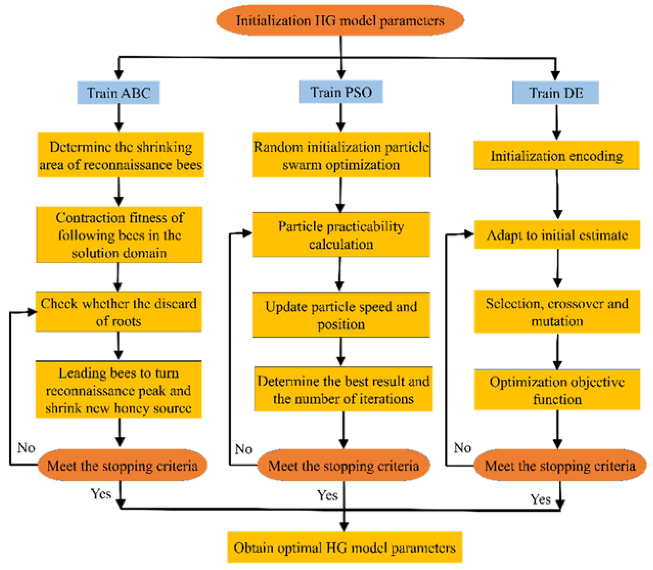
2.4. Parameter Optimization Process

Equation (6) is reasonable in form for different types of climate regions, but many studies have found that these coefficients are different in regions with completely opposite climate conditions [48]. Therefore, the three parameters in the Hargreaves model need to be regionally corrected, and the original results should be kept as brief as possible.

The ABC, DE and PSO optimization algorithms are used to correct the above three parameters (C, m and a), requiring some specific steps for the proper correction of the Hargreaves model such as

(1)

Divide the calibration period and inspection period. The continuous daily meteorological data of each station, in this case, are divided into two parts used as calibration samples (L₁) and validation samples (L₂).

(2)

Determine the feasible region of the variable to be optimized. After analysis and debugging, the three parameters for this article were respectively taken: $C\in \left[5\times {10}^{-5},0.02\right]$, m $\in \left[0.02,2.0\right]$ and $a\in \left[2.0,85.0\right]$.

(3)

Determine the optimization objective function. To ensure that the Hargreaves model has high simulation accuracy and generalization ability at the same time after correction, the minimization of the following function F is taken as the optimization objective of the three optimization algorithms.

$$F=\frac{L_1}{L_1+L_2}\left(1-C_{D1}\right)+\frac{L_2}{L_1+L_2}\left(1-C_{D2}\right)$$

(17)

where C_D1 and C_D2 represent the Nash–Sutcliffe coefficients of the periodic rate and the inspection period respectively, and the calculation formulas used in this case are:

$$C_{D1}=1-\frac{{\sum }_{t=1}^{L_1}{[E{T}_H\left(t\right)-E{T}_0\left(t\right)]}^2}{{\sum }_{t=1}^{L_1}{[E{T}_0\left(t\right)-E{T}_{0mean}]}^2}$$

(18)

$$C_{D2}=1-\frac{{\sum }_{t=1}^{L_1+L_2}{[E{T}_H\left(t\right)-E{T}_0\left(t\right)]}^2}{{\sum }_{t=L_1+1}^{L_1+L_2}{[E{T}_0\left(t\right)-E{T}_{0mean}]}^2}$$

(19)

where ET_H(t) and ET₀(t) are the ET₀ of calculated by Hargreaves and PM formulas, and ET₀ represents the value of ET₀(t).

(4)

The ABC, DE and PSO optimize methods are used with the Hargreaves model to find the minimum value of F function. The undetermined parameters are C, m, a, and the search interval are determined in the second step. The FAO recommended values are 0.0023, 17.8 and 0.5, respectively. When the F function is the smallest, the convergence is the best and the optimal result is output. The specific optimization process is shown below Figure 2:

2.5. Performance Evaluation

The determination coefficient (R²), relative root mean square error (RRMSE), mean absolute error (MAE), and Nash–Sutcliffe coefficient (NS) were used to evaluate performances of the models [38,48].

$$R^2=\frac{{\sum }_{i=1}^n{\left(E{T}_i^M-E{T}_i^{PM}\right)}^2}{{\sum }_{i=1}^n{\left(E{T}_i^M-E{T}_{0,mean}\right)}^2·{\sum }_{i=1}^n{\left(E{T}_i^{PM}-E{T}_{0,mean}\right)}^2}$$

(20)

$$RRMSE=\frac{RMSE}{E{T}_{0,mean}}=\sqrt{\frac{1}{n}{\displaystyle \sum }_{i=1}^n{(E{T}_i^M-E{T}_i^{PM})}^2}$$

(21)

$$MAE=\frac{{\sum }_{i=1}^n\left|E{T}_i^M-E{T}_i^{PM}\right|}{n}$$

(22)

$$NS=1-\frac{{\sum }_{i=1}^n{(E{T}_i^M-E{T}_i^{PM})}^2}{{\sum }_{i=1}^n{(E{T}_i^{PM}-E{T}_{i,mean})}^2}$$

(23)

Following the above equation, $E{T}_i^{PM}$ and $E{T}_i^M$ are ET₀ values at the i-th step obtained by PM and HG models, respectively. n is the number of the time steps and ET_0,mean is the value of the PM calculation. The RRMSE is dimensionless, with the value from 0 (the perfect fit) to ∞ (the worst fit). The MAE is measured in mm/d, with the value from 0 (the perfect fit) to ∞ (the worst fit). The NS is also dimensionless, and its value also ranges from 1 (the perfect fit) to −∞ (the worst fit).

We adopted the Global Performance Index (GPI) to combine the results of all the above indicators and avoid the difference of individual indicators [49]. Such an index can be calculated as

$$GP{I}_i={\displaystyle \sum }_{j=1}^4{\alpha }_j\left(y_j-y_{ij}\right)$$

(24)

where R² and NS are the main indicators with ${\alpha }_j$ equal to −1. For other indicators, ${\alpha }_j$ is equal to 1, y_j is the median value of the scale value of index j, y_ij stands for the scale value of index j of model i. The GPI value gets higher according to the accuracy of the model.

3. Results

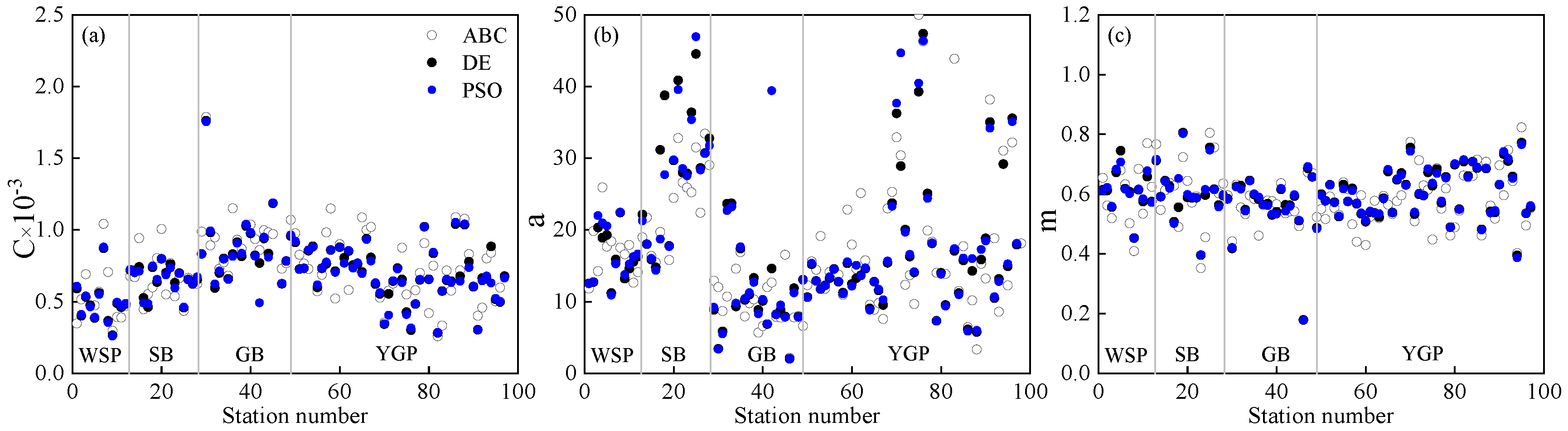
3.1. Calibration of Hargreaves

The distribution of three empirical parameters (C, a, m) of the HG model after calibration based on ABC, DE and PSO algorithms is shown in Figure 3a–c. The parameter C, a and m deviate from the FAO recommended values (C = 0.0023, a = 17.8, m = 0.5) at most stations. The parameter C value is higher than 0.0023, only lower than the recommended value in a few stations. After optimization, ABC, DE and PSO algorithms are concentrated in [0.25 × 10⁻³, 0.30 × 10⁻³], [0.26 × 10⁻³, 0.31 × 10⁻³], and [0.28 × 10⁻³, 0.30 × 10⁻³], respectively. Parameter C is highest in GB, and it is overall a little lower in NSP and YGP than that in SB and GB. The geographical difference of parameter a is easily spotted, and after the optimization of the three algorithms, the main distribution intervals are [2.16, 42.23], [2.00, 46.03] and [2.00, 44.50]. The changes are large in the NSP and the YGP, and the difference between the optimization results in the SB and the GB is small. The parameter m is also slightly affected by regional differences. Moreover, the calibrated value of the three optimization algorithms is slightly higher than the recommended value of 0.5. In this case, the main distribution intervals are [0.18, 0.82], [0.17, 0.80] and [0.18, 0.80], and the difference among optimization results is insignificant. Overall, the YGP and the NSP showed complex topographic structures with large undulations. The parameter a is greatly affected by regional differences, followed by the parameter c, and the parameter m that is basically not touched by the terrain undulations, indicating that the accuracy of the HG model is mainly influenced by parameter a.

Based on ABC, DE and PSO optimization algorithm, the average values of parameters C, m and a in HG model in Southwest (SW) China are displayed in

Table 2. The average value of calibrated parameters in the HG model in the southwestern regions based on the ABC, DE and PSO optimization algorithms.

Zone	ABC			DE			PSO
	C × 10−3	m	a	C × 10−3	m	a	C × 10−3	m	a
SW	0.75	0.58	19.13	0.73	0.60	17.90	0.72	0.60	18.90
NSP	0.53	0.60	29.14	0.49	0.59	32.13	0.58	0.56	32.91
YGP	0.71	0.58	20.18	0.70	0.60	17.79	0.69	0.60	18.68
GB	1.06	0.55	9.69	1.00	0.56	10.68	0.99	0.56	11.86
SB	0.66	0.61	17.14	0.66	0.62	16.47	0.65	0.62	16.80

Note: the recommended values of C, m and a by FAO are 2.3 × 10⁻³, 0.5 and 17.8. NSP: Northwest Sichuan Plateau; SB: Sichuan Basin; YGP: Yunnan–Guizhou Plateau; GB: Guangxi Basin; SW: Southwest.

. It can be concluded that the parameter c calibrated in the 4 regions of the SW of the three optimization algorithms is larger in the GB, and the difference between the other regions is small. The change of the parameter m is not much and is closer to the FAO recommended value of 0.50. The parameter a fluctuation range is also larger in the NSP, but smaller in the GB.

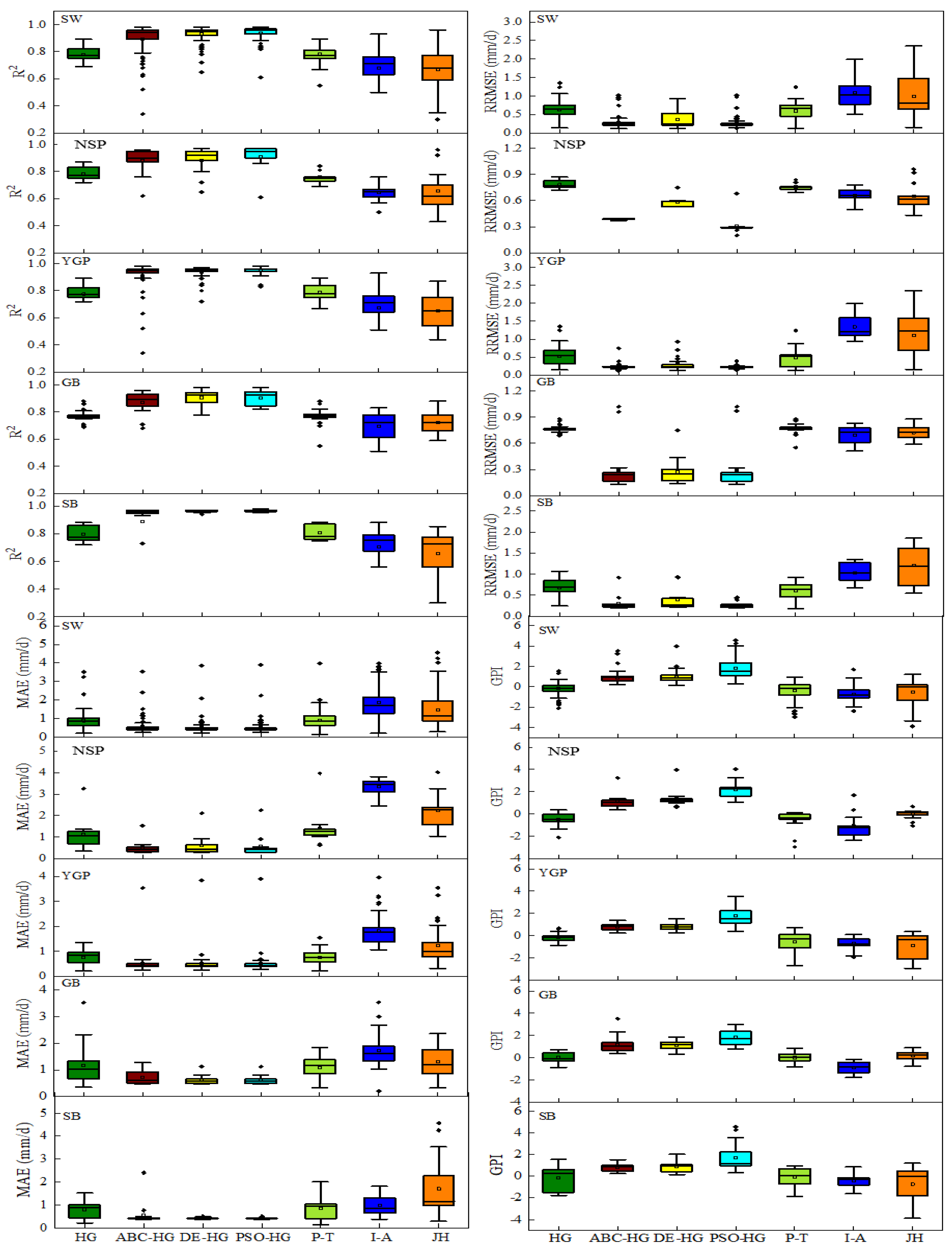
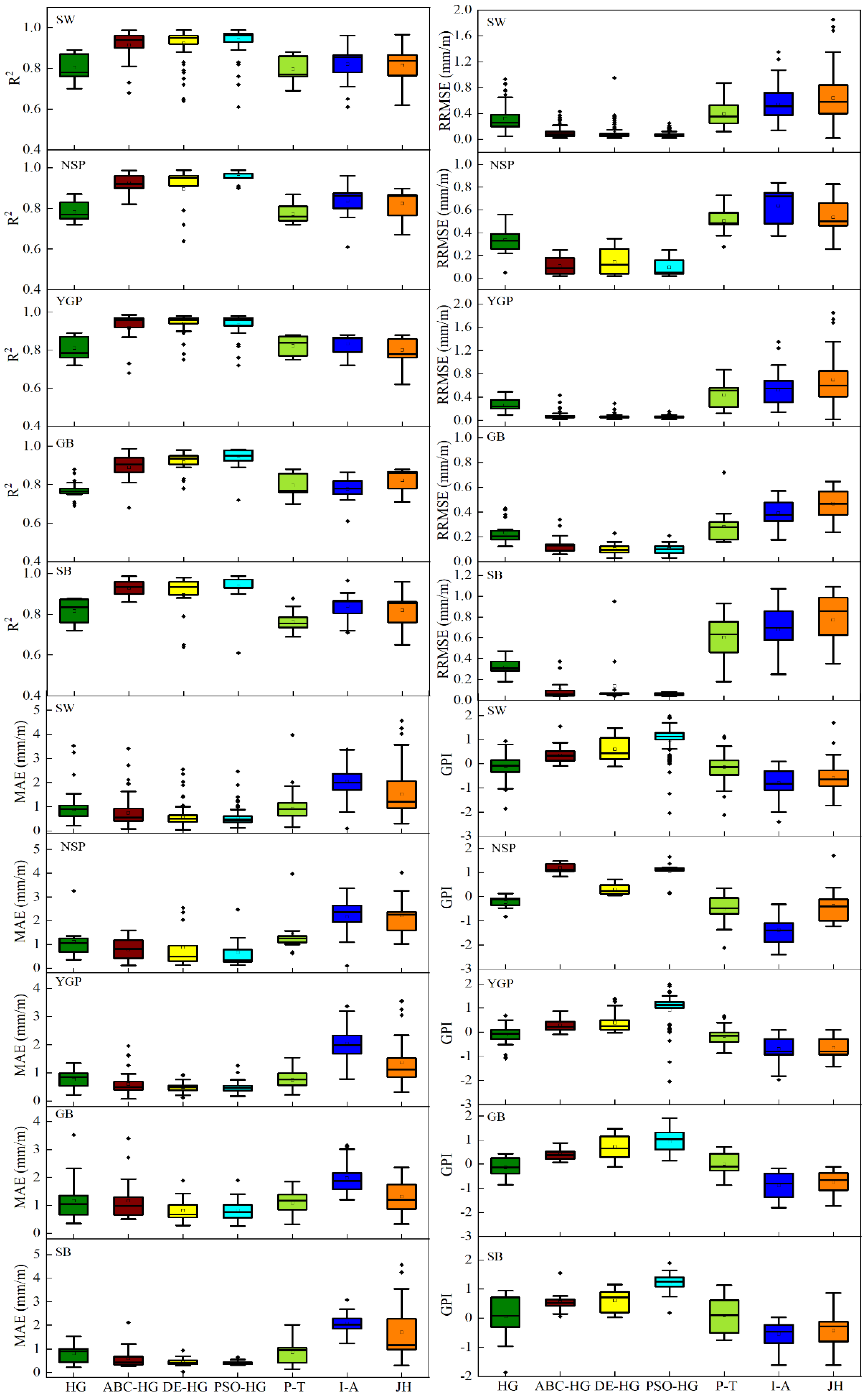
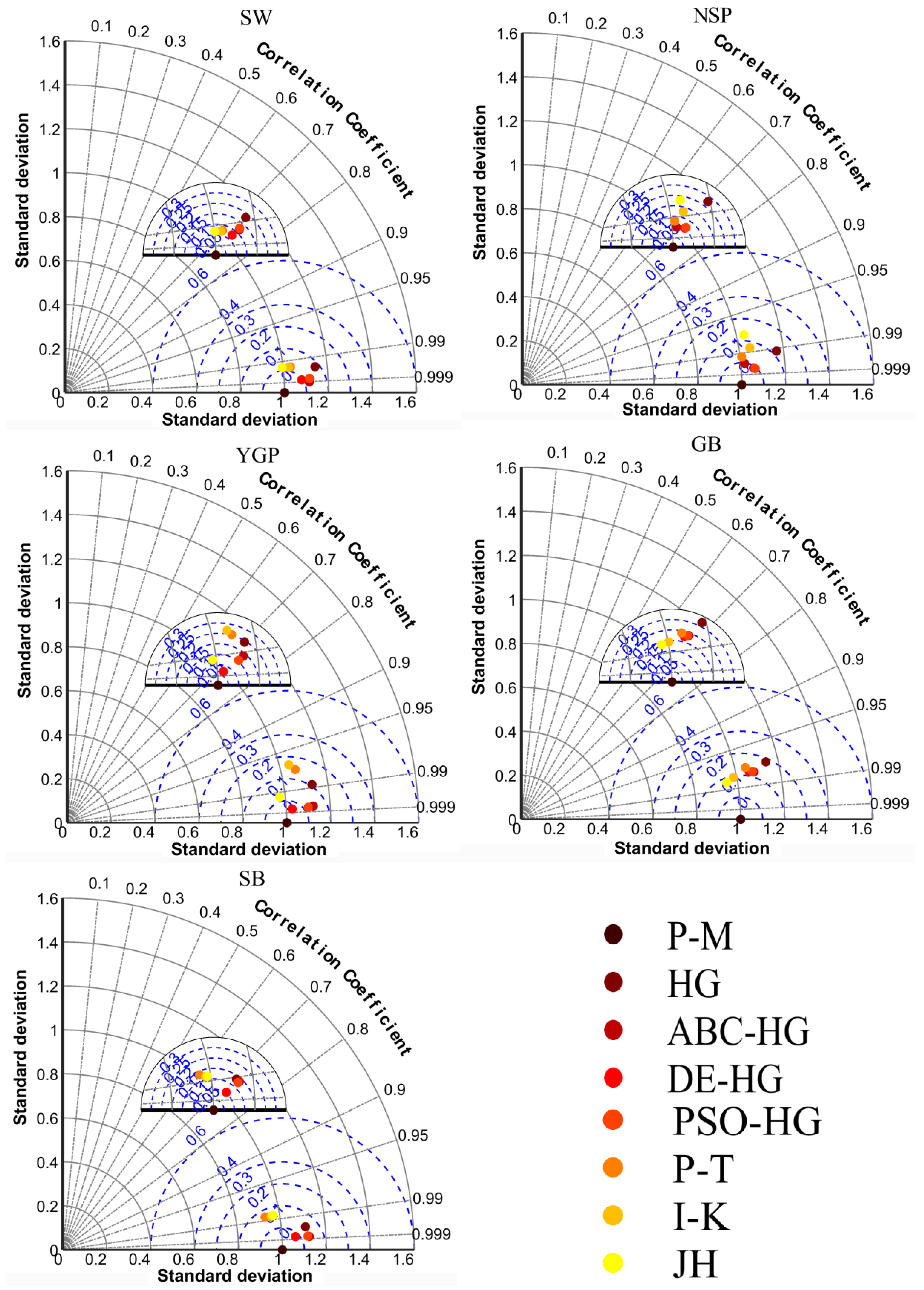
3.2. Performances of HG Models on a Daily Basis

The accuracy of daily ET₀ estimated by seven models in Southwest China and four regions is represented in

Table 3. The daily ET₀ accuracy estimated based on ABC, DE and PSO optimization algorithms in Southwest China.

Sub-Zone	Statistical Indicator	HG	ABC-HG	DE-HG	PSO-HG	P-T	I-A	JH
SW	R2	0.79	0.82	0.82	0.83	0.77	0.79	0.67
	RRMSE (mm/d)	0.48	0.25	0.25	0.24	0.78	0.48	1.91
	MAE (mm/d)	0.90	0.55	0.57	0.52	1.52	0.91	2.92
	GPI	−0.16	0.13	0.04	0.14	−0.54	−0.24	−1.04
	Rank	4	2	3	1	6	5	7
NSP	R2	0.78	0.83	0.83	0.83	0.67	0.76	0.64
	RRMSE (mm/d)	0.59	0.27	0.30	0.25	1.76	0.67	1.98
	MAE (mm/d)	1.11	0.55	0.58	0.51	3.19	1.39	3.22
	GPI	−0.47	−0.22	−0.25	−0.03	−1.07	−0.52	−3.17
	Rank	4	2	3	1	6	5	7
SB	R2	0.83	0.85	0.86	0.86	0.84	0.79	0.75
	RRMSE (mm/d)	0.31	0.29	0.23	0.23	0.30	0.46	0.91
	MAE (mm/d)	0.81	0.57	0.43	0.42	0.75	0.85	1.70
	GPI	−0.16	−0.01	0.22	0.26	−0.12	−0.36	−0.42
	Rank	5	3	2	1	4	6	7
YGB	R2	0.78	0.82	0.82	0.82	0.76	0.79	0.64
	RRMSE (mm/d)	0.44	0.24	0.24	0.23	1.91	0.42	2.05
	MAE (mm/d)	0.75	0.55	0.57	0.54	2.12	0.75	3.35
	GPI	−0.08	0.00	−0.04	0.07	−0.12	−0.07	−0.51
	Rank	5	2	3	1	6	4	7
GB	R2	0.77	0.79	0.79	0.80	0.69	0.77	0.72
	RRMSE (mm/d)	0.55	0.24	0.28	0.21	1.77	0.57	0.67
	MAE (mm/d)	1.09	0.60	0.72	0.51	5.09	1.09	1.32
	GPI	0.06	0.36	0.24	0.41	−0.55	0.00	−0.05
	Rank	4	2	3	1	7	5	6

Note: HG, PT, IA and JH represent Hargreaves, Priestley–Taylor, Imark–Allen and Jensen–Haise respectively. NSP: Northwest Sichuan Plateau; SB: Sichuan Basin; YGP: Yunnan–Guizhou Plateau; GB: Guangxi Basin; SW: Southwest.

. Observing the results, it can be said that in the Southwest region, the optimization models (ABC-HG, DE-HG and PSO-HG) are more accurate than 4 empirical models (HG, PT, IA and JH) and the PSO-HG model is the one with the highest accuracy. In SW area, PSO-HG model had the highest accuracy, followed by ABC-HG and DE-HG models, and R² of ET_0-PSO-GH, ET_0-ABC-GH and ET_0-DE-GH were 0.83, 0.83 and 0.82; RRMSE were 0.24 mm/d, 0.25 mm/d and 0.25 mm/d; MAE were 0.52 mm/d, 0.55 mm/d and 0.57 mm/d and GPI marked 0.14, 0.13 and 0.04, respectively. In the NSP area, PSO-HG model had the highest accuracy, followed by ABC-HG and DE-HG models, and R² of ET_0-PSO-GH, ET_0-ABC-GH. ET_0-DE-GH were 0.83, 0.83 and 0.83; RRMSE were 0.25 mm/d, 0.27 mm/d and 0.30 mm/d; MAE were 0.51 mm/d, 0.55 mm/d and 0.58 mm/d and GPI were −0.03, −0.22 and −0.25, respectively.

Regarding the YGB area, PSO-HG model also had the highest accuracy, followed by ABC-HG and DE-HG models, and R² of ET_0-PSO-GH, ET_0-ABC-GH and ET_0-DE-GH were 0.82, 0.82 and 0.82; RRMSE were 0.23 mm/d, 0.23 mm/d and 0.24 mm/d; MAE were 0.54 mm/d, 0.55 mm/d and 0.57mm/d and GPI were 0.07, 0.00 and −0.04, respectively. In GB area, PSO-HG model was also the most assertive one, followed by ABC-HG and DE-HG models, and R² of ET_0-PSO-GH, ET_0-ABC-GH and ET_0-DE-GH were 0.80, 0.79 and 0.79; RRMSE were 0.21 mm/d, 0.24 mm/d and 0.28 mm/d; MAE were 0.51 mm/d, 0.60 mm/d and 0.72 mm/d and GPI marked 0.41, 0.36 and 0.24, respectively. In SB area, PSO-HG model was again the one with the highest accuracy, followed by DE-HG and ABC-HG models, and R² of ET_0-PSO-GH, ET_0-ABC-GH and ET_0-DE-GH, in this case, were 0.86, 0.86 and 0.85, RRMSE were 0.23 mm/d, 0.23 mm/d and 0.29 mm/d, MAE were 0.42 mm/d, 0.43 mm/d and 0.57 mm/d and GPI were 0.26, 0.22 and −0.01, respectively. Among the three optimization algorithms, the PSO algorithm was the one with the highest accuracy after calibration, because the particle speed determines the direction and distance of the particle movement in it, and its speed is dynamically adjusted according to the movement experience and other particles, to achieve the individual that does the best in the solvable space. Therefore, it is suggested to use PSO-HG model to estimate the daily ET₀ of Southwest China and four regions, since it was the one with more accurate events in all the examinations.

Based on the HG model calibrated by ABC, DE and PSO optimization algorithms and 4 empirical models, the daily ET₀ accuracy indexes estimated in SW, NSP, YGP, GB and SB regions are represented in Figure 4. As it can be seen, on a daily scale, the median lines range of R², RRMSE and MAE values of ET_0-ABC-GH value in southwest areas ranged from 0.89 to 0.96 (average value 0.93), 0.23 to 0.91 mm/d (average value 0.41 mm/d) and 0.42 to 0.60 mm/d (average value 0.47 mm/d), respectively. The ET_0-DE-GH values were from 0.92 to 0.97 (average value 0.94), 0.23 to 0.59 mm/d (average value 0.31) and 0.41 to 0.58 mm/d (average value 0.46) in R², RRMSE and MAE values in various regions of Southwest China. The ET_0-PSO-GH values were between 0.93 and 0.97 (average value 0.95), 0.23 and 0.29mm/d (average value 0.25) and 0.41 and 0.58 mm/d (average value 0.46) in R², RRMSE and MAE values in various regions of Southwest China. The accuracy of the 4 empirical models in various regions of Southwest China were median line ranges of R², RRMSE and MAE hit 0.62–0.78 (average value 0.73), 0.81–1.37 mm/d (average value 0.53 mm/d) and 0.75–3.46 mm/d (average value 1.29 mm/d), respectively. According to the GPI estimated by all models, the accuracy of PSO-HG model was the highest in the whole southwest region, followed by ABC-HG and DE-HG model, with median lines of 1.54, 0.94 and 0.91, respectively. However, the accuracy of the JH model was relatively low, followed by HG and I-A models, with median lines of −0.79, 0.13 and −0.12. In summary, the accuracy of the optimized HG model in the southwestern region was higher than the empirical model, and the accuracy of the PSO-HG model is higher than the other models.

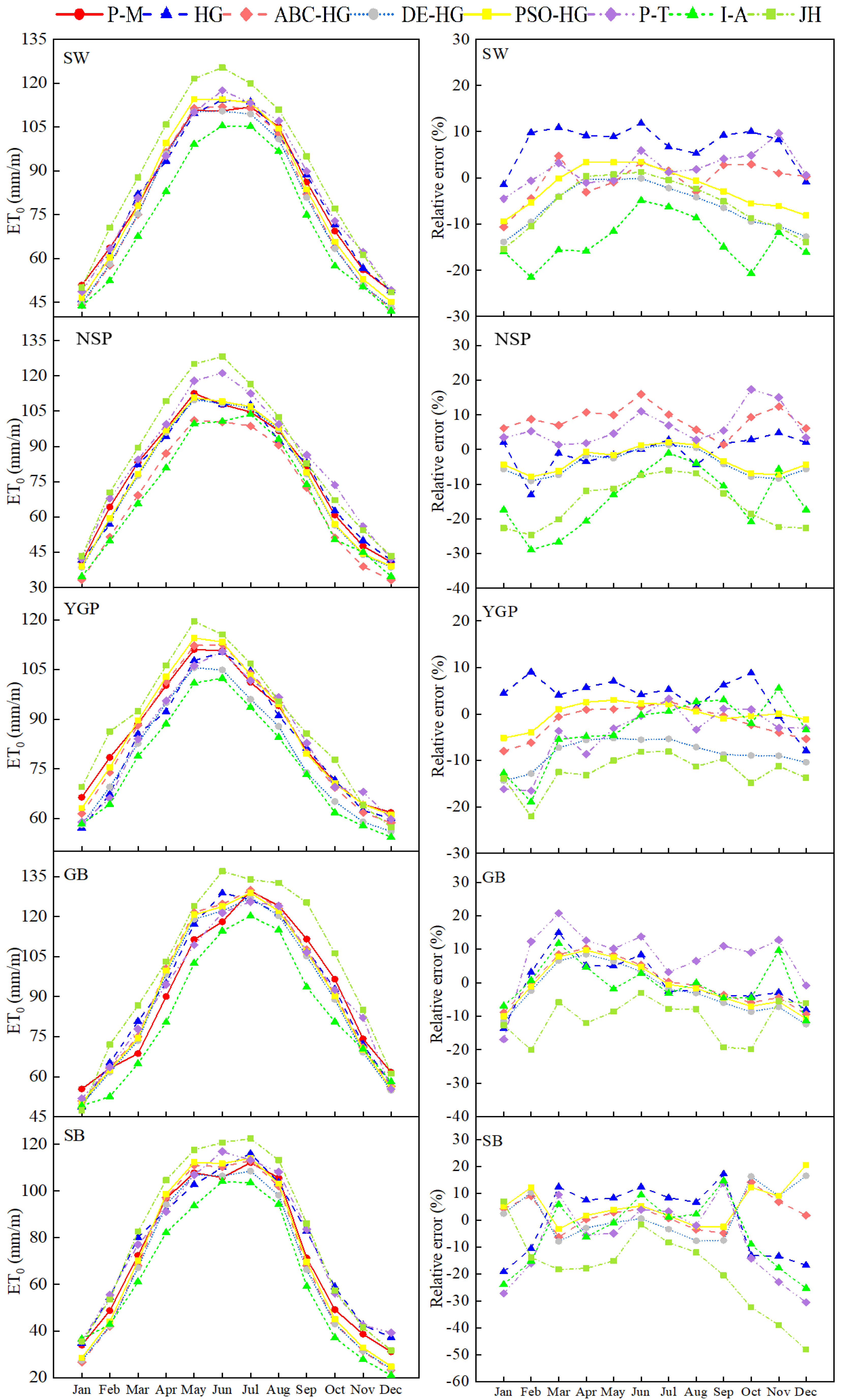
3.3. Performances of HG Models on a Monthly Basis

Based on ABC, DE and PSO optimization algorithms, the monthly average ET₀ estimated in Southwest China and the four regions are properly explained in Figure 5 and the monthly average ET₀ estimated by different models showed a parabolic change. For SW, NSP, SB, GB and YGP, the error range of HG model calibrated by optimization algorithm a were 15.40 to 3.40%, −28.17 to 2.10%, −14.32 to 3.01%, −33.75 to 5.42% and −12.41 to 10.76%. Also, the error ranges of 4 empirical models were −21.51 to 11.81%, −51.95 to 17.33%, −22.04 to 9.07%, −48.09 to 20.68% and −20.09 to 20.70%. These results showed that the accuracy of the HG model improved by the optimization algorithm in estimating monthly scale ET₀ and it was obviously better than that of the commonly used empirical model. In addition, the accuracy of the estimated monthly ET₀ of the seven models during the period from May to September was relatively high and the relative errors in SW, NSP, SB, GB and YGP were lower than 11.80%, 11.01%, 7.05%, 4.92% and 5.06%, respectively, which may be due to the complex topographic structure of the southwest region and the small difference in surface temperature. The 4 empirical models had higher accuracy in summer and lower accuracy in winter, because the terrain structure there is complex, and winter is mostly cloudy and rainy. On the YGP, the terrain structure is mostly karst landforms, caused by the different degrees of soil evaporation, which leads to differences in relative humidity. Overall, the PSO-HG model had the highest accuracy of ET₀ estimated by SW, NSP, YGB, SB and GB, with average relative errors of −2.69%, 3.48%, −1.64%, 6.10% and −0.92%. Therefore, the PSO-HG model might be the best fit to estimate monthly scale ET₀ in Southwest China.

Based on ABC, DE and PSO optimization algorithms, the monthly average ET₀ estimated in Southwest China and the four regions are properly explained in Figure 5 and the monthly average ET₀ estimated by different models showed a parabolic change. For SW, NSP, SB, GB and YGP, the error range of HG model calibrated by optimization algorithm a were 15.40 to 3.40%, −28.17 to 2.10%, −14.32 to 3.01%, −33.75 to 5.42% and −12.41 to 10.76%. Also, the error ranges of 4 empirical models were −21.51 to 11.81%, −51.95 to 17.33%, −22.04 to 9.07%, −48.09 to 20.68% and −20.09 to 20.70%. These results showed that the accuracy of the HG model improved by the optimization algorithm in estimating monthly scale ET₀ and it was obviously better than that of the commonly used empirical model. In addition, the accuracy of the estimated monthly ET₀ of the seven models during the period from May to September was relatively high and the relative errors in SW, NSP, SB, GB and YGP were lower than 11.80%, 11.01%, 7.05%, 4.92% and 5.06%, respectively, which may be due to the complex topographic structure of the southwest region and the small difference in surface temperature. The 4 empirical models had higher accuracy in summer and lower accuracy in winter, because the terrain structure there is complex, and winter is mostly cloudy and rainy. On the YGP, the terrain structure is mostly karst landforms, caused by the different degrees of soil evaporation, which leads to differences in relative humidity. Overall, the PSO-HG model had the highest accuracy of ET₀ estimated by SW, NSP, YGB, SB and GB, with average relative errors of −2.69%, 3.48%, −1.64%, 6.10% and −0.92%. Therefore, the PSO-HG model might be the best fit to estimate monthly scale ET₀ in Southwest China.

Figure 6 is based on the HG model calibrated by ABC, DE and PSO algorithms and 4 empirical models, which showed the monthly ET₀ accuracy index estimated in the SW, NSP, YGP, GB and SB. On the monthly scale, the median line range of R², RRMSE and MAE of the ET_0-ABC-GH value in different regions of Southwest China were 0.91–0.96 (average value 0.93), 0.06–0.13 mm/m (average value 0.08) and 0.43–0.98 mm/m (average value 0.65), respectively. Adding to that, the median lines of ET_0-DE-GH value were 0.94–0.96 mm/m (average value 0.95), 0.06–0.12 mm/m (average value 0.08) and 0.42–0.67 mm/m (average value 0.51) and the median lines of ET_0-PSO-GH value hit 0.95–0.97 (average value 0.96), 0.05–0.10 mm/m (average value 0.08), and 0.34–0.75 mm/m (average value 0.48). When it comes to the accuracy of the 4 empirical models in each region in the southwest region, the median lines of R², RRMSE and MAE were 0.75–0.86 (average value 0.80), 0.21–0.72 mm/m (average value 0.43 mm/m) and 0.76–2.25 mm/m (average value 1.12 mm/m). According to the GPI estimated by all models, the PSO-HG model was the most assertive one, followed by the ABC-HG and DE-HG models, with median lines that marked 1.13, 0.47 and 0.35, respectively. However, the JH model showed lower accuracy, followed by IA, P-T and HG model, with median lines as −0.82, −0.64, −0.04 and 0.02, respectively. Hence, in the southwest region, the accuracy of the optimized HG model is higher than that of the empirical model, and the accuracy of the PSO-HG model surpasses the other models. Figure 7 shows Taylor diagrams that represent the relationship among the standard deviation, root mean square error, and determination coefficient of each model, and intuitively shows the estimated monthly ET₀ accuracy of the 7 models at each weather station site. This also shows that the monthly ET₀ estimated by the PSO-HG model is the most precise one.

4. Discussion

This research found that a model improved via an intelligent optimization algorithm has a higher estimation accuracy than that of the original empirical models. The optimized HG models overcome the errors caused by topographical and climate factors (temperature, air pressure, and radiation), which possess regional characteristics that it could make corresponding adjustments in different elevations, topographic structures and land types, making its accuracy significantly improved. Wu et al. [49] used four models optimized by intelligent optimization algorithms (GA, ACO, CSA and FPA) to estimate the daily ET₀ in different climate zones in China, and found a significant improvement in estimating values of daily ET₀ in the temperate monsoon and (sub) tropical monsoon climates with the models optimized by the four algorithms, while the RMSE decreased by 14.0%, 25.1%, 31.4% and 33.1%, respectively. Additionally, under temperate continental and mountainous plateau climates, the RMSE also declined by 5.2%, 9.8%, 12.9% and 14.1%, respectively. Still in this realm, Hai et al. [50] studied 3 stations in Burkina Faso to get a better algorithm to improve the fuzzy model to predict regional daily ET₀ and found that the estimation accuracy of the optimized hybrid model was revamped significantly. Based on the original model, and under the complete input of meteorological data, the RMSE value was between 0.24 and 0.40 mm/d, and the R² value was between 0.95 and 0.97. Yin et al. [51] used a genetic algorithm to optimize support vector machine hybrid model to predict ET₀ in China arid areas, and the results showed that the RMSE and R² values of the support vector machine model upgraded by this new algorithm were 0.138 mm/d and 0.995 respectively using complete meteorological data. Its accuracy was also improved by about 10%, compared with the original support vector machine model. Fan et al. [52] used support vector machine firefly calculation (SVM-FFA), Copula based nonlinear quantile regression (CNQR) and empirical model to estimate daily radiation. The findings from this process showed that, compared with CNQR, the average SVMFFA decreased by 0.67% (0.01 MJ·m²/d), and the average R² increased by 0.43% (0.004 MJ·m²/d). As to the training time of the three methods, the calculation time of SVM-FFA (1.68 s) was less than that of CNQR (6.68 s), but the parameter optimization time of SVM-FFA (4.91 s) marked 105 times that of CNQR. However, some scholars think that the accuracy of the optimized models has not improved compared to traditional models [53]. The reasons for this phenomenon might be that in some biologically inspired algorithms coupled with the model course or in the optimization process, it may fall into a local optimum, resulting in the lower accuracy than the original model. Besides that, it may be that when the model is boosted, the level of the researcher subjective judgment involved in the parameter adjustment process affects the final prediction progress of the model.

It was found that the PSO-HG model has the highest accuracy in estimating ET₀, followed by ABC-HG and DE-HG models. The main difference between PSO, ABC and DE optimization algorithms lies in the global convergence process of parameter calibration. The PSO optimization algorithms use nonlinear changes to adjust the samples, while ABC optimization algorithms adopt the dynamic adjustment. DE optimization algorithms involve crossover, mutation and selection operations, which helps to improve the performance accuracy of the model. It revamps the model parameters by looking for the optimal parameter solution by the nonlinear fitting. Therefore, the principle of the PSO algorithm is consistent with the nature of finding the optimal frameworks.

5. Conclusions

In this paper, we used ABC, DE and PSO optimization algorithms based on meteorological data obtained from 98 stations from 1961 to 1991 improve the HG model for estimating ET₀ in Southwest China. The meteorological data from 1992 to 2019 was checked to evaluate the applicability of the calibrated HG model, HG model, PT model, Imark–Allen model, and JH model on different time scales, and it helped to shape some conclusions.

(1)

On daily scale, the calibrated HG models were more accurate compared with the 4 physical models for daily ET₀ estimation at the 4 sub-zones of southwest China. Among them, PSO-HG model showed the highest accuracy in NSP, YGB, SB and GB, with average R² of 0.83, 0.82, 0.80 and 0.86, average RRMSE of 0.25 mm/d, 0.23 mm/d, 0.23 mm/d and 0.21 mm/d, and average MAE of 0.25 mm/d, 0.23 mm/d, 0.23 mm/d and 0.21 mm/d, and GPI of −0.03, 0.07, 0.26 and 0.41, respectively. In SW research region, the PSO-HG model had the best estimation accuracy for daily ET₀, followed by ABC-HG and DE-HG models, with average R² of 0.83, 0.82 and 0.82, average RRMSE of 0.24 mm/d, 0.25 mm/d and 0.25 mm/d, average MAE of 0.52 mm/d, 0.57 mm/d and 0.55 mm/d, and average GPI of 0.14, 0.13 and 0.04, respectively.

(2)

On a monthly scale, the calibrated HG model (RE < 18%) showed a better performance than the 4 physical models (RE > 18%) at the 4 sub-zones. PSO-HG model showed the best performance for ET_0-mad estimation in NSP, YGB, SB and GB, with average RE of 3.48%, −1.64%, 6.10% and −0.92%. In SW research region, the PSO-HG model showed the best performance for ET_0-mad estimation, followed by ABC-HG and DE-HG model, with R² median of 0.96, 0.95 and 0.94, RRMSE median of 0.16 mm/m, 0.17 mm/m and 0.18 mm/m, MAE median of 0.46 mm/m, 0.50 mm/m and 0.55 mm/m, and GPI median of 1.13, 0.47 and 0.35, respectively.

(3)

In the southwest humid region, the HG model calibrated by the optimization algorithms is compared with the HG, PT, Imark–Allen and JH model. It can be said that the ET₀ estimated by optimized models has higher accuracy, and the PSO-HG model has the highest estimation accuracy. Based on these outcomes, PSO-HG model can be accurately recommended to estimate the southwest humid ET₀ accurately.

References

1. Fan, J.; Wu, L.; Zhang, F. Climate change effects on reference crop evapotranspiration across different climatic zones of China during 1956–2015. J. Hydrol. 2016, 542, 923–937. [Google Scholar] [CrossRef]
2. Gao, Z.D.; He, J.S.; Dong, K.B.; Bian, X.D.; Li, X. Sensitivity study of reference crop evapotranspiration during growing season in the West Liao River basin, China. Theor. Appl. Climatol. 2016, 124, 865–881. [Google Scholar] [CrossRef]
3. Granata, F. Evapotranspiration evaluation models based on machine learning algorithms—A comparative study. Agric. Water Manag. 2019, 217, 303–315. [Google Scholar] [CrossRef]
4. Shiri, J.; Kisi, O.; Landeras, G.; Lopez, J.J.; Nazemi, A.H.; Stuyt, L.C.P.M. Daily reference evapotranspiration modeling by using genetic programming approach in the Basque Country (Northern Spain). J. Hydrol. 2012, 414, 302–316. [Google Scholar] [CrossRef]
5. Abdullah, S.S.A.; Malek, M.A.; Abdullah, N.S.; Kisi, O.; Yap, K.S. Extreme learning machines: A new approach for prediction of reference evapotranspiration. J. Hydrol. 2015, 527, 184–195. [Google Scholar] [CrossRef]
6. Allen, R.G.; Pereira, L.S.; Raes, D.; Smith, M. Crop Evapotranspiration. Guide Lines for Computing Crop Evapotranspiration; FAO Irrigation and Drainage: Rome, Italy, 1998; p. 56. [Google Scholar]
7. Han, H.; Bai, Y.; Zhang, X. Study on applicabilities and modifications of several methods for estimating reference crop evapotranspiration in Guizhou Province. Water Resour. Hydropower Eng. 2018, 10, 198–204. [Google Scholar]
8. Ai, Z.; Yang, Y. Modification and Validation of Priestley-Taylor Model for Estimating Cotton Evapotranspiration under Plastic Mulch Condition. J. Hydrometeorol. 2016, 17, 1281–1293. [Google Scholar] [CrossRef]
9. Rivero, M.; Orozco, S.; Sellschopp, F.S.; Loera-Palomo, R. A new methodology to extend the validity of the Hargreaves-Samani model to estimate global solar radiation in different climates: Case study Mexico. Renew. Energy 2017, 114, 1340–1352. [Google Scholar] [CrossRef]
10. Jabulani, J. Evaluation of the potential of using the modified Jensen-Haise model as an irrigation scheduling technique in Zimbabwe. Electron. J. Environ. Agric. Food Chem. 2008, 7, 2771–2778. [Google Scholar]
11. Zhang, Q.; Cui, N.; Yu, F. Improvement of Makkink model for reference evapotranspiration estimation using temperature data in Northwest China. J. Hydrol. 2018, 566, 264–273. [Google Scholar]
12. Yang, Y.; Cui, Y.; Bai, K. Short-term forecasting of daily reference evapotranspiration using the reduced-set Penman-Monteith model and public weather forecasts. Agric. Water Manag. 2019, 211, 70–80. [Google Scholar] [CrossRef]
13. Didari, S.; Ahmadi, S.H. Calibration and evaluation of the FAO56-Penman-Monteith, FAO24-radiation, and Priestly-Taylor reference evapotranspiration models using the spatially measured solar radiation across a large arid and semi-arid area in southern Iran. Theor. Appl. Climatol. 2019, 136, 441–445. [Google Scholar] [CrossRef]
14. Pretheep-Kumar, P.; Tilak, M.; Durairasu, P. A model for predicting the infestation of mealybugs in jatropha based on the weather parameters. Int. J. Agric. 2013, 3, 608–619. [Google Scholar]
15. Mendicino, G.; Senatore, A. Regionalization of the Hargreaves coefficient for the assessment of distributed reference evapotranspiration in Southern Italy. J. Irrig. Drain. Eng. 2013, 139, 349–362. [Google Scholar] [CrossRef]
16. Virginia, G.; Phillip, B.; Clifford, E. A Bayesian Dynamic Method to Estimate the Thermophysical Properties of Building Elements in All Seasons, Orientations and with Reduced Error. Energies 2018, 11, 802. [Google Scholar]
17. Cui, W.; Sun, Z.; Yang, J. The temperature model of the thermal re-radiation model in multilayer insulation systems. Open Astron. 2020, 29, 32–39. [Google Scholar] [CrossRef]
18. Antwerpen, H.J.V.; Greyvenstein, G.P. Evaluation of a detailed radiation heat transfer model in a high temperature reactor systems simulation model. Nucl. Eng. Des. 2008, 238, 2985–2994. [Google Scholar] [CrossRef]
19. Irwan, Y.M.; Daut, I.; Safwati, I. An Estimation of Solar Characteristic in Kelantan Using Hargreaves Model. Energy Procedia 2013, 36, 473–478. [Google Scholar] [CrossRef] [Green Version]
20. Valiantzas, J.D. Temperature-and humidity-based simplified Penman’s ET0 formulae. Comparisons with temperature-based Hargreaves-Samani and other methodologies. Agric. Water Manag. 2018, 208, 326–334. [Google Scholar] [CrossRef]
21. Almorox, J.; Elisei, V.; Aguirre, M.E. Calibration of Hargreaves model to estimate reference evapotranspiration in Coronel Dorrego, Argentina. Rev. Fac. Cienc. Agrar. 2012, 44, 101–109. [Google Scholar]
22. Liu, X.-Y.; Li, Y.-Z.; Zhong, X.-L. Evaluation of 16 reference crop evapotranspiration (ET0) models based on daily measured values of weighing lysimeter. Agrometeorol. China 2017, 38, 278–291. [Google Scholar]
23. Almorox, J.; Grieser, J. Calibration of the Hargreaves–Samani method for the calculation of reference evapotranspiration in different Kppen climate classes. Hydrol. Res. 2016, 47, 521–531. [Google Scholar] [CrossRef] [Green Version]
24. Feng, Y.; Cui, N.; Gong, D.; Zhang, Q.; Zhao, L. Evaluation of random forests and generalized regression neural networks for daily reference evapotranspiration modeling. Agric. Water Manag. 2017, 193, 163–173. [Google Scholar] [CrossRef]
25. Feng, Y.; Jia, Y.; Zhang, Q.; Gong, D.; Cui, N. National-scale assessment of pan evaporation models across different climatic zones of China. J. Hydrol. 2018, 564, 314–328. [Google Scholar] [CrossRef]
26. Zhu, B.; Feng, Y.; Gong, D. Hybrid particle swarm optimization with extreme learning machine for daily reference evapotranspiration prediction from limited climatic data. Comput. Electron. Agric. 2020, 173, 105430. [Google Scholar] [CrossRef]
27. Martí, P.; Gonzalez-Altozano, P.; Lopez-Urrea, R.; Mancha, L.A.; Shiri, J. Modeling reference evapotranspiration with calculated targets. Assessment and implications. Agric. Water Manag. 2015, 149, 81–90. [Google Scholar] [CrossRef]
28. Martí, P.; Zarzo, M.; Vanderlinden, K.; Girona, J. Parametric expressions for the adjusted Hargreaves coefficient in Eastern Spain. J. Hydrol. 2015, 529, 1713–1724. [Google Scholar] [CrossRef]
29. Talaee, P.H. Performance evaluation of modified versions of Hargreaves equation across a wide range of Iranian climates. Meteorol. Atmos. Phys. 2014, 126, 65–70. [Google Scholar] [CrossRef]
30. Martinez, C.A.; Tejero, J.M. A wind-based qualitative calibration of the Hargreaves ET 0 estimation equation in semiarid regions. Agric. Water Manag. 2004, 64, 251–264. [Google Scholar] [CrossRef] [Green Version]
31. Yang, Y.H.; Zhang, Z.Y. Method for calculating Lhasa reference crop evapotranspiration by modifying Hargreaves. Adv. Water Sci. 2009, 20, 614–618. (In Chinese) [Google Scholar]
32. Perera, K.C.; Andrew, W.W.; Bandara, N.; Biju, G. Forecasting daily reference evapotranspiration for Australia using numerical weather prediction outputs. Agric. For. Meteorol. 2014, 194, 50–63. [Google Scholar] [CrossRef]
33. Nakayama, K.; Pruitt, W.O.; Chandio, B.A. Some Aspects of the Priestley and Taylor Model to Estimate Evapotranspiration. Tech. Bull. Fac. Hortic. Chiba Univ. 1983, 32, 25–30. [Google Scholar]
34. Irmak, S.; Irmak, A.; Allen, R.G.; Jones, J.W. Solar and net radiation-based equations to estimate reference evapotranspiration in humid climate. J. Irrig. Drain. Eng. 2003, 129, 336–347. [Google Scholar] [CrossRef]
35. Jensen, M.E.; Haise, H.R. Estimating evapotranspiration from solar radiation. J. Irrig. Drain. Eng. 1963, 89, 15–41. [Google Scholar]
36. Samani, Z. Estimating solar radiation and evapotranspiration using minimum climatological data. J. Irrig. Drain. Eng. 2000, 126, 265–267. [Google Scholar] [CrossRef]
37. Trajkovic, S. Hargreaves versus Penman-Monteith under Humid conditions. J. Irrig. Drain. Eng. 2007, 133, 38–42. [Google Scholar] [CrossRef]
38. Feng, Y.; Jia, Y.; Cui, N. Calibration of Hargreaves model for reference evapotranspiration estimation in Sichuan basin of southwest China. Agric. Water Manag. 2017, 181, 1–9. [Google Scholar] [CrossRef]
39. Shao, P.; Yang, L.; Tan, L. Enhancing artificial bee colony algorithm using refraction principle. Soft Comput. 2020, 24, 15291–15306. [Google Scholar] [CrossRef]
40. Wu, Y.; Xu, J.; Zhang, C. A Heuristic Scout Search Mechanism for Artificial Bee Colony Algorithm. In Advances in Natural Computation, Fuzzy Systems and Knowledge Discovery; Springer: Cham, Switzerland, 2019; pp. 271–278. [Google Scholar]
41. Wu, B.; Qian, C.; Ni, W. Hybrid harmony search and artificial bee colony algorithm for global optimization problems. Comput. Math. Appl. 2012, 64, 2621–2634. [Google Scholar] [CrossRef] [Green Version]
42. Ozkan, C.; Kisi, O.; Akay, B. Neural networks with artificial bee colony algorithm for modeling daily reference evapotranspiration. Irrig. Sci. 2011, 29, 431–441. [Google Scholar] [CrossRef]
43. Storn, R.; Price, K. Differential Evolution–A Simple and Efficient Heuristic for global Optimization over Continuous Spaces. J. Glob. Optim. 1997, 11, 341–359. [Google Scholar] [CrossRef]
44. Roman, P. Application of the Differential Evolution for simulation of the linear optical response of photosynthetic pigments. J. Comput. Phys. 2018, 372, 603–615. [Google Scholar]
45. Shi, Y. Particle swarm optimization: Developments, applications and resources. In Proceedings of the 2001 Congress on Evolutionary Computation (IEEE Cat. No.01TH8546), Seoul, Korea, 27–30 May 2001. [Google Scholar]
46. Robinson, J.; Rahmat-Samii, Y. Particle swarm optimization in electromagnetics. IEEE Trans. Antennas Propag. 2004, 52, 397–407. [Google Scholar] [CrossRef]
47. Fan, J.; Wu, L.; Ma, X.; Zhou, H.; Zhang, F. Hybrid support vector machines with heuristic algorithms for prediction of daily diffuse solar radiation in air-polluted regions. Renew. Energy 2020, 145, 2034–2045. [Google Scholar] [CrossRef]
48. Despotovic, M.; Nedic, V.; Despotovic, D.; Cvetanovic, S. Review and statistical analysis of different global solar radiation sunshine models. Renew. Sustain. Energy Rev. 2015, 52, 1869–1880. [Google Scholar] [CrossRef]
49. Wu, L. Daily reference evapotranspiration prediction based on hybridized extreme learning machine model with bio-inspired optimization algorithms: Application in contrasting climates of China. J. Hydrol. 2019, 577, 123960. [Google Scholar] [CrossRef]
50. Hai, T.; Lamine, D.; Ansoumana, B. Reference evapotranspiration prediction using hybridized fuzzy model with firefly algorithm: Regional case study in Burkina Faso. Agric. Water Manag. 2018, 208, 140–151. [Google Scholar]
51. Yin, Z.; Wen, X.; Feng, Q.; He, Z.; Zou, S.; Yang, L. Integrating genetic algorithm and support vector machine for modeling daily reference evapotranspiration in a semi-arid mountain area. Hydrol. Res. 2017, 48, 1177–1191. [Google Scholar] [CrossRef]
52. Fan, J.; Yue, W.; Wu, L. Evaluation of SVM, ELM and four tree-based ensemble models for predicting daily reference evapotranspiration using limited meteorological data in different climates of China. Agric. For. Meteorol. 2018, 263, 225–241. [Google Scholar]
53. Shamshirband, S.; Amirmojahedi, M.; Gocić, M.; Akib, S.; Petković, D.; Piri, J.; Trajkovic, S. Estimation of reference evapotranspiration using neural networks and cuckoo search algorithm. J. Irrig. Drain. Eng. 2015, 142, 04015044. [Google Scholar] [CrossRef]
Figure 1. Map of weather stations distribution of 4 regions in Southwest China. NSP: Northwest Sichuan Plateau; SB: Sichuan Basin; YGP: Yunnan–Guizhou Plateau; GB: Guangxi Basin.
Atmosphere 12 00015 g001
Figure 2. The flow chart of ABC, DE and PSO optimization methods process.
Atmosphere 12 00015 g002
Figure 3. (ac) Calibration results of HG model empirical parameter (C, a, m) based on the ABC, DE and PSO optimization methods. Note, NSP: Northwest Sichuan Plateau; SB: Guangxi Basin; GB: Sichuan Basin; YGP: Yunnan–Guizhou Plateau.
Atmosphere 12 00015 g003
Figure 4. Based on ABC, DE and PSO algorithms, HG model and four empirical models are calibrated to estimate daily ET0 accuracy of stations in Southwest China and four regions. Note: HG, PT, IA and JH represent Hargreaves, Priestley–Taylor, Imark–Allen and Jensen–Hais, respectively. NSP: Northwest Sichuan Plateau; GB: Guangxi Basin; SB: Sichuan Basin; YGP: Yunnan–Guizhou Plateau.
Atmosphere 12 00015 g004
Figure 5. Comparison of the accuracy of the monthly average evapotranspiration estimation model in the southwest and the 4 sub-regions.
Atmosphere 12 00015 g005
Figure 6. Estimated monthly ET0 accuracy in Southwest China and 4 districts based on HG model calibrated by ABC, DE, and PSO algorithms and 4 empirical models. Note: HG, PT, IA and JH represent Hargreaves, Priestley–Taylor, Imark–Allen and Jensen–Hais. NSP: Northwest Sichuan Plateau; GB: Guangxi Basin; SB: Sichuan Basin; YGP: Yunnan–Guizhou Plateau.
Atmosphere 12 00015 g006
Figure 7. Taylor diagram of estimated monthly ET0 accuracy in Southwest China and 4 districts based on HG model calibrated by ABC, DE, and PSO algorithms and 4 empirical models. Note: HG, PT, IA and JH represent Hargreaves, Priestley–Taylor, Imark–Allen and Jensen–Hais, respectively. NSP: Northwest Sichuan Plateau; GB: Guangxi Basin; SB: Sichuan Basin; YGP: Yunnan–Guizhou Plateau.
Atmosphere 12 00015 g007