The Relationship of Energy and CO₂ Emissions with GDP per Capita in Colombia

Abstract

We analyze the relationship of CO₂ emissions per capita and primary energy per capita with gross domestic product (GDP) per capita and other relevant variables in Colombia for the period 1971–2017. Two partial adjustment models are estimated through the seemingly unrelated regression equations method. There is a decrease in these environmental pressures during some years of the period. However, the results reject the environmental Kuznets curve hypothesis and indicate that economic growth is still linked to an increase in these environmental pressures in Colombia. Moreover, a linear relationship between both indicators and GDP per capita is not rejected. Several factors explain the changes in energy consumption and emissions over time, the policies applied being crucial. Some determinants that helped to control these environmental pressures are the change in primary energy source composition, which entailed primary energy savings and a reduction in CO₂ emissions, as well as the regulations aimed at controlling CO₂ emissions from the transport and industrial sectors.

1. Introduction

The share of the contribution of developing countries and emerging economies to total emissions has steadily increased in last decades. Moreover, even though some developed countries have managed to limit emissions growth, the increase experienced in developing countries has led to a constant increase in global greenhouse gas emissions. Consequently, the analysis of the determinants of emissions in developing countries is crucial in the challenge of mitigating global greenhouse gas emissions. Moreover, the energy and environmental policies that may lead to curb fossil fuel consumption and emissions growth in these countries are also essential. Of special interest is the study of how these countries could decouple their economic development and social welfare from the consumption of fossil fuels and associated emissions. In this paper, we study whether this was the case for Colombia and analyze the determinants of the trajectories of energy consumption and CO₂ emissions during the period considered. These findings could provide important insights into the measures allowing more sustainable growth in developing countries.

The Colombian economy was greatly affected by a strong energy crisis during 1992–1993, caused by the El Niño phenomenon. This led the government to develop an Energy Emergency Plan and periodically formulate energy supply and diversification strategies promoting the use of more sustainable energy sources (Law 693 of 2001 and Law 939 of 2004). In addition, at the end of 1992, the new Public and Electric Utilities laws of the Political Constitution of 1991 were introduced [1]. This impulse to develop a cleaner energy sector continues at present. The Development Plan 2015–2018 had among its purposes to move towards low-carbon sustainable growth through the use of clean and unconventional sources of energy [2].

The trajectory of the use of primary energy in Colombia between 1971 and 2017 showed a significant increase (a 176.9% increase in the period). However, the use of primary energy experienced a decrease during the period 1996–2002 (except for a spike in 1998). During the whole period, the use of primary energy from natural gas and hydroelectric plants increased by 778.0% and 822.0%, respectively, while the use of petroleum products and coal “only” increased by 132.9% and 113.8%, respectively [3]. These elements contributed together to moderate the increase in total primary energy consumption and CO₂ emissions. The greater weight of natural gas, to the detriment of the most polluting fossil fuels, would largely explain the behavior of carbon dioxide (CO₂) emissions, which decreased from 1.52 t CO₂ per capita in 1997 to 1.22 t CO₂ per capita in 2004, and did not recover to the 1997 value until 2013. While the non-Organization for Economic Co-operation and Development (OECD) American region experienced a 46.6% increase in CO₂ emissions per capita (from 1.46 to 2.14 tons per capita) between 1997 and 2017, Colombia had lower emissions per capita and its increase was more moderate (from 1.18 to 1.53 tons per capita, a 30.1% increase) [4]. In the same period there was significant and continuous economic growth in Colombia, with an average annual rate of 3.9% in the period 1971–2017; only in 1999 was there a negative rate of growth of −4.2%. Moreover, according to [5,6] the Colombian economy has experienced changes in its productive structure towards tertiarization. It would then be interesting to analyze the relationship between the changes in the consumption of some energy sources (and associated emissions) and the behavior of economic activity.

The interest in analyzing the relationship between economy and energy increased at the beginning of the 1970s due to the oil crisis and its impact on the global economy. Later, at the beginning of the 1990s, several studies suggested that for some polluting substances there was a delinking of economic growth from a certain level of income per capita [7,8], a relationship that is known as the environmental Kuznets curve (EKC) hypothesis. This finding led some authors to argue that the solution to environmental problems was just to promote growth [9]. However, most subsequent studies dismissed this option and highlighted the need for environmental policies, as well as the role played by these in the cases in which such delinking occurred [8,10,11]. The results in the literature are varied, finding evidence for and against the EKC hypothesis; it is less clear that the hypothesis is fulfilled for pollutants with long-term effects, such as CO₂ [12,13,14]. Moreover, most studies that found evidence in favor of the hypothesis obtained turning points above the average income level of most countries, and especially of the average income level of developing countries.

Most of the first papers on the issue analyzed the hypothesis for groups of countries with panel or cross-sectional data. However, several authors suggest that it is more appropriate to conduct studies at the country level in order to develop a more in-depth analysis of the relationship that occurs in each case [13,15,16,17]. Individual analyses would also be more appropriate given the empirical evidence that the relationship between environmental degradation and per capita income may be different for different countries in aspects such as functional form, parameters, and turning points [16,17].

The present work aims to improve the knowledge of the relationships between energy, CO₂ emissions, and economic activity, so as to contribute to a better planning of energy use and emissions control without harming economic development (a requirement expressed in the National Energy Plan 2006–2025 and in the Plan Visión Colombia 2019). In short, we are going to investigate the following: the relationships of GDP per capita with per capita energy consumption and CO₂ emissions in Colombia, during the period 1971–2017, testing the EKC hypothesis as well as the significance of other variables for these environmental pressures. To address these objectives, a partial adjustment model (PAM) is estimated for both energy and CO₂ emissions through the seemingly unrelated regression equations (SURE) method. Unlike previous studies on Colombia that used static equations [18], a contribution of our paper is that dynamic equations are used, and different variables are considered besides income. In addition, our analysis extends over a long period of almost five decades. The paper will provide evidence for the case of a developing Latin American country, a region for which evidence is still scarce. It will also provide insights into these relationships and the policies that may help to make possible a more sustainable development in Colombia and in countries with a similar economic context. The rest of this paper is organized as follows. Section 2 provides a brief conceptual and empirical reference framework for the relationships between the level of economic activity and environmental pressures. Section 3 explains the data sources, the methods, and the specification of the models estimated. Section 4 presents and discusses the results. Section 5 presents the conclusions.

2. Conceptual and Empirical Review

The EKC hypothesis posits the existence of an inverted U-shaped relationship between environmental degradation and per capita income. The EKC owes its name to its analogy with the Kuznets curve, which reflects the relationship found by Kuznets [19] between the level of per capita income and inequality [20]. Among the pioneering works, [7,8,21] found some evidence of an inverted U-shaped relationship between economic growth and some polluting substances, while [22] presented various graphs showing this type of relationship for some indicators of environmental quality.

According to this hypothesis, the initial phase of economic development of a country is characterized by the development of industry and polluting extractive activities, so that emissions increase as production increases. In the second phase, a certain threshold (turning point) is reached, from which economic growth allows the adoption of new, less polluting technologies and, in addition, increases the share of the services sector (supposedly less polluting) (however, some service activities are highly polluting [23], as is the case of transport, or require inputs from highly polluting activities, so that they would be indirectly responsible for their emissions [24,25]. Hence, it cannot be conclusively stated that the tertiarization of an economy necessarily implies a lower environmental impact) and information-intensive industries [7,21]. Moreover, the higher per capita income could translate into a greater preference for environmental quality [26,27,28,29]. Even though in some cases there is a delinking between environmental pressure and economic growth, as suggested by the EKC, this could be a temporary situation, as [30] state, so there could be a later re-linking (due to the possible exhaustion of mitigation opportunities), converting additional growth into environmental degradation. These authors also distinguish two forms of de-linking or dematerialization in a growing economy: weak (relative) dematerialization and strong (absolute) dematerialization. The first is characterized by decreasing the intensity of use of materials or waste per unit of production. The second means that the total environmental pressure decreases over time. In terms of environmental impact, the important thing is to analyze whether or not a strong dematerialization occurs.

In the literature, multiple determinants of emissions have been analyzed in addition to income, such as, the inequality of power and wealth [31,32,33], the structure of the energy supply [13,34], the degree of urbanization [35,36,37], the composition of production [35,38,39,40], openness to foreign trade [12,21,38,40,41,42,43,44,45], foreign finance [46], or even less “conventional” determinants, such as the degree of trust [47] or corruption [43], among others. However, given the number of possible determining factors and their possible correlations, authors often decide to directly relate the environmental pressure with the GDP per capita, so that the whole of the (apparent) direct and indirect relations established between both variables through different channels is taken into account [17]. In any case, most studies emphasize that among the fundamental elements that influence the relationship between economic growth and environmental degradation are the public policies enforced [10,14,22,26,30,39,48,49]. The importance of the quality of policies and institutions for reducing environmental degradation at low income levels and accelerating improvements at high income levels is highlighted in [10,39].

Several studies have found that the relationship between economic growth and environmental degradation can take different forms, depending on the type of pollutant, the database, the period analyzed, the model specifications, and the methods used, so that although the EKC hypothesis could reflect what happens in some cases, the empirical evidence would not be too favorable as a general explanation of the relationship between economic growth and environmental degradation.

There are varied results in the literature. Some studies find that some countries during certain periods fulfill the EKC for some pollutants [7,12,21,50,51]. In other studies there is contradictory evidence for the same pollutants [51,52], depending on the region analyzed and the estimated model. Other studies have found evidence contrary to the EKC hypothesis [13,35,38,39,51,53,54,55,56] for the environmental pressure indicators studied. The studies employ different econometric methods. In contrast to the first studies, in many post-1995 studies the problems of autocorrelation and heteroskedasticity were corrected for and consistency and simultaneity tests were carried out to avoid errors of bias depending on the estimation technique used. Specifically, in the case of time series models, the hypothesis of non-cointegration between GDP and emissions were tested [38].

Much of the literature that finds evidence favorable for the EKC hypothesis was carried out with cross-sectional data, where the models estimated assume homogeneity in the form of the relationship between emissions and GDP for the different countries and in its parameters and, therefore, the turning point in the relationship. However, this assumption of homogeneity was rejected when empirically tested [16,17]. It seems, therefore, that studies of individual countries that go into more depth about the relationship that occurs in each case would make more sense. This would be the case of, for example, the studies for Austria [38], China [57], Sweden [58], Malaysia [59], Spain [13,23,56], and Uruguay [40], among others.

The patterns of the relationship between income and environmental degradation depend on the economic structure, access to technology, public policies and trade, as well as environmental regulation, among other possible factors. Hence, the way the country has faced the oil crises and the policy measures that have been adopted to improve energy efficiency become highly relevant issues that we consider in our research.

3. Data, Methods, and Model Specification

3.1. Data

The data used for the estimates come from the International Energy Agency [3,4]. CO₂ emissions are measured in millions of tons, population in millions of inhabitants, gross domestic product (GDP) in billions of 2010 US dollars (USD) in purchasing power parity (PPP) values, and the total supply of primary energy and of the different sources of primary energy are measured in thousands of tons of oil equivalent (ktoes). The data cover the period 1971–2017.

3.2. Methods

We first graphically analyze the behavior of the data, studying whether the data apparently show weak (emissions or energy per unit of GDP) or strong (CO₂ emissions or per capita energy) decoupling from GDP per capita. To do this, we produce various scatter plots and draw trend lines showing both linear and a polynomial least squares regressions between the variables for the analysis period, which allows observing the pattern of behavior of the data and identifying the types of relationships between the variables over time. We then proceed to the estimation of a PAM that allows observing in a more interactive way the trajectory of the variables over time, taking into account different determinants, as well as identifying the functional form of the relationship

Previous studies have used the PAM to analyze electricity demand [60,61], as well as different polluting emissions [15,62]. Our study is the first to apply this method to the analysis of environmental pressures in the Colombian case.

The use of the PAM allows us to analyze the relationships between the variables: (i) identifying if there has been a change in the parameters of the model and estimating the equilibrium equations; (ii) estimating the influence of income and some socioeconomic variables on the environmental pressure indicator; (iii) considering the past evolution of environmental pressure as a possible influence on the present (the reason may be technological, psychological, or institutional); (iv) examining the speed with which the changes take place. This is achieved by calculating the elasticities. The short-run ones capture the change in the rates of use of the existing flow and the long-run ones capture both changes in the rate of use as well as changes in the economic structure.

We estimate the PAM equations with the SURE method in order to obtain better estimations. Given the potentially correlated errors of both equations, the SURE method provides more efficient estimators. This correlation may be caused by similar omitted variables in both equations, which seems quite plausible. Appendix B provides a proof of the greater efficiency of employing SURE for our estimation.

3.3. Specification of the Model

According to the model, the dependent variable, Y_t (CO₂ emissions per capita or primary energy per capita in a given year) depends on X_t, a vector of different socioeconomic factors or other variables (GDP per capita, regulation, and energy structure) that influence Y_t, α is the intercept, β is the vector, X_t are the coefficients of the explanatory variables, and u_t is the error term:

$$Y_t^{*}=\alpha +\beta X_t+u_t$$

(1)

The adjustment process can be represented as:

$$\underset{\mathrm{Observed} \mathrm{change}}{\underbrace{Y_t-Y_{t-1}}}=\lambda \underset{\begin{array}{l}\mathrm{Desired} \mathrm{change}=\\ =\mathrm{long} \mathrm{run} \mathrm{change}\end{array}}{\underbrace{\left(Y_t^{*}-Y_{t-1}\right)}}$$

(2)

The equation specifies that the change observed in the environmental pressure indicator at any time t, is a fraction λ of the long-run change, where λ is the adjustment coefficient. It is assumed that the coefficient is between 1 and 0. The closer to 1 the coefficient, the higher the speed of the adjustment.

Two models are estimated, one for the use of energy and the other for CO₂ emissions. We take the series in logarithms, so that the coefficients are interpreted as elasticities.

In model 1, the equation estimated for energy is

$$\ln \left(\frac{P{E}_t}{PO{P}_t}\right)={\beta }_0+{\beta }_1\ln \left(\frac{GD{P}_t}{PO{P}_t}\right)+{\beta }_2{\left[\ln \left(\frac{GD{P}_t}{PO{P}_t}\right)\right]}^2+{\beta }_3\left[\ln \left(\frac{PE\_N{G}_t+PE\_HIDR{O}_t}{EP\_TOTA{L}_t}\right)\right]+\left(1-\lambda \right)\ln \left(\frac{P{E}_{t-1}}{PO{P}_{t-1}}\right)$$

(3)

where the lagged dependent variable measures the relationship that energy consumption has with the one in the previous period and makes the model dynamic. The GDP per capita coefficient measures the impact of the scale of production, while, according to its usual interpretation in the EKC literature, the squared variable shows the endogenous change in the relationship as the income level increases due to changes in the productive structure, consumption patterns, and technology, among other determinants. The EKC hypothesis is met if the variable in levels has a positive value and the squared variable has a negative one [7,21]. The coefficient of the proportion of natural gas plus hydroelectric energy in total primary energy $\left(\frac{{P{E}_{NG}}_t+{P{E}_{HIDRO}}_t}{{P{E}_{TOTAL}}_t}\right)$ reflects the impact of a change in the composition of energy sources towards sources that are more efficient in their transformation into final energy. These are the two main primary sources of electricity generation in the country. Both contribute to a lower energy consumption due to their high efficiency in the transformation of primary energy to final energy [63].

In model 2, the equation estimated for CO₂ emissions is

$$\ln \left(\frac{C{O}_{2t}}{PO{P}_t}\right)={\beta }_0+{\beta }_1\ln \left(\frac{GD{P}_t}{PO{P}_t}\right)+{\beta }_2{\left[\ln \left(\frac{GD{P}_t}{PO{P}_t}\right)\right]}^2+{\beta }_3\left[\ln \left(\frac{PE\_REN{O}_t}{EP\_TOTA{L}_t}\right)\right]+{\beta }_4{G}_t+\left(1-\lambda \right)\ln \left(\frac{C{O}_2{}_{t-1}}{PO{P}_{t-1}}\right)$$

(4)

As in the previous model, the lagged dependent variable makes the model dynamic and shows the relationship between the current generation of emissions and that in the previous period. The proportion of renewable energy in total primary energy, $\left(\frac{{P{E}_{RENO}}_t}{{E{P}_{TOTAL}}_t}\right)$, made up mainly of hydroelectricity, biofuels, solar, and wind, are clean energies that would contribute to a lower generation of CO₂ emissions per capita. For example, in Colombia, sugarcane ethanol is associated with a 71% reduction in emissions [64]. The variable G_t is a proxy variable for regulation, since factors related to changes in legislation can affect environmental quality [65]. It is a dichotomous variable that takes the value zero before 1998 and one after 1998. Some Colombian government regulations related to the control of environmental pollution include (a) Decree 948 of 1995 that establishes standards for air quality control and establishes different progressive quotas especially from 1998. (b) Decree 1228 of 1997 that determines emission regulations for automotive vehicles. (c) Resolution 619 of 1997 that establishes atmospheric emission permits for certain industries and activities with fixed emission sources. (d) Laws 693 and 697 of 2001: the first promotes the rational use of energy and the second creates incentives to use biofuels to reduce emissions.

4. Results

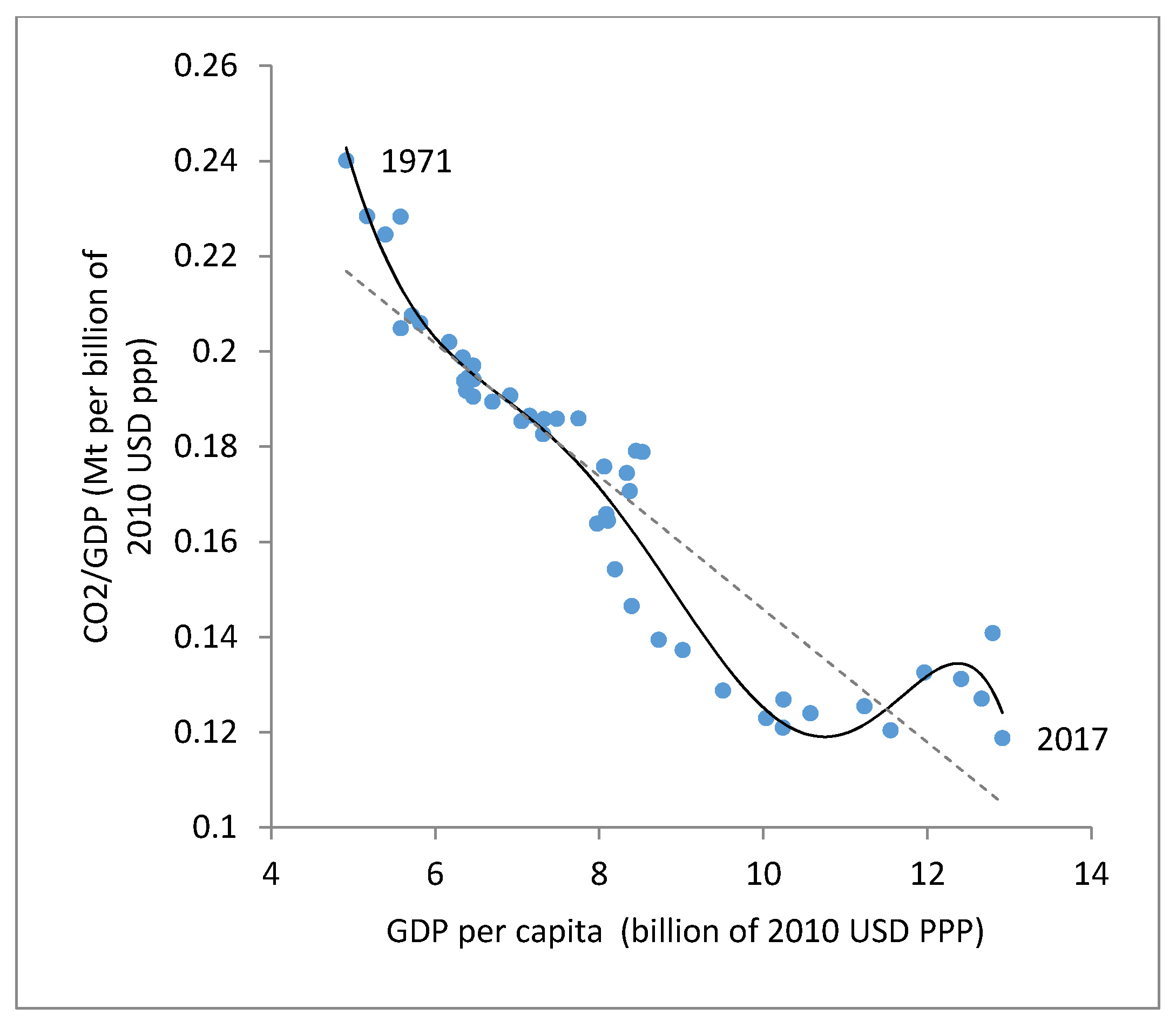
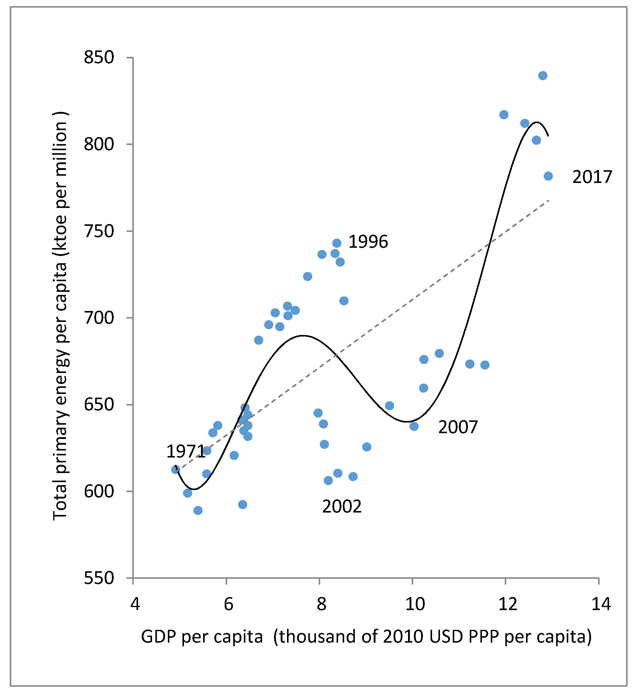
4.1. Graphical Analysis of the Relationships between Energy or CO₂ Emissions and GDP in Colombia

We carry out a graphical analysis of the relationships between energy consumption, emission generation, and GDP per capita. This allows observing whether there is any type of (weak/relative or strong/absolute) delinking with respect to energy consumption and CO₂ emissions. Figure 1 shows the relationship between energy per unit of product and GDP per capita. This shows a negative correlation between the variables, indicating that, as GDP per capita increases, there is a decrease in energy per unit of output. That is to say, there is an apparent relative delinking (weak dematerialization) between energy and economic growth. This delinking, however, is not so clear since 2007, as the energy intensity does not decrease much after this year. Figure 2 shows a relatively similar behavior when analyzing the relationship between CO₂ emissions per unit of product and GDP per capita, while the negative relationship is even less clear in this case after 2007.

As shown by Figure 3, there seem to be two changes in the relationship between primary energy per capita and GDP per capita. First, the relationship between energy per capita and GDP per capita changes from a strongly positive correlation during the period 1971–1996 to a negative correlation during 1996–2007, whereas after 2007, the correlation is again positive until almost the end of the period. Figure 4 shows a similar behavior for the relationship between CO₂ emissions per capita and GDP per capita, with some differences in the intensity, with the difference that, in this case, the first change occurs a period later. Then, there seems to be a negative correlation between emissions and economic growth during 1997–2007.

In both Figure 3 and Figure 4, we observe a complex relationship between GDP per capita and energy and CO₂ emissions. If the period ended in the year 2007 (or even in the year 2010), the relationships shown in the figure would resemble an inverted-U shape, which would be consistent with the EKC hypothesis, as there is a decrease in energy consumption together with greater GDP after the year 1996, while the same happens for CO₂ emissions after the year 1997.

This means that, as of 1996 and 1997, the consumption of energy and the generation of CO₂ emissions, respectively, present an apparently absolute delinking from economic growth (dematerialization), since the increase in GDP does not seem to entail greater emissions of CO₂, nor higher energy consumption. However, the figures show a later re-association, which is very clear after 2007, of the ratio of GDP to primary energy consumption and CO₂ emissions. Actually, primary energy consumption starts to increase with GDP after 2002, while CO₂ emissions do so after 2004. This re-linking is particularly sharp after the year 2011 in the case of CO₂ emissions per capita and 2010 in the case of energy consumption per capita. Therefore, there is not an absolute delinking between these environmental pressures and GDP for the period 1997–2017. This is also confirmed by the linear relationship between the variables shown by the dashed line.

According to the literature on the EKC, the reasons most commonly used to justify a decoupling, such as that observed for these few years, are technological changes and structural changes [15,21], in addition to (or as a result of) the enforced policies. In the case of Colombia, these changes could have occurred and interacted with other factors, generating modifications in the composition of the energy sources and the intensity of the use of the materials leading to the behavior observed in the environmental variables considered. However, the changes experienced have not been enough to make compatible the subsequent increase in production with lower levels of emissions and energy consumption, as we observe a clear re-linking between economic growth and these environmental pressures. Next, we estimate a PAM to analyze in greater detail the relationships between the variables and the influential factors.

4.2. Results of the Econometric Estimations

Models 1 (Equation (3)) and 2 (Equation (4)) are estimated for energy consumption per capita and CO₂ emissions per capita, respectively.

We estimated the PAM equations with the SURE method in order to obtain more efficient estimations, given the potentially correlated errors of both equations.

Table 1. Short-run estimates of models 1 and 2.

	Short-Run Coefficient	Standard Error	t-Statistic	p-Value
Model 1 (dependent variable ln(PEt/POPt))
Intercept	1.10	0.64	1.73	0.0880 *
ln(GDPt/POPt)	0.92	0.46	2.00	0.0486 **
(ln(GDPt/POPt))2	−0.14	0.10	−1.45	0.1514
ln((PE_GNt+PE_HIDROt)/PE_TOTALt)	−0.18	0.05	−3.86	0.0002 ***
ln(PEt−1/POPt−1)	0.60	0.08	7.17	0.0000 ***
Model 2 (dependent variable ln(CO2t/POPt))
Intercept	−0.10	0.36	−0.27	0.7893
ln(GDPt/POPt)	−0.32	0.34	−0.94	0.3481
(ln(GDPt/POPt))2	0.12	0.08	1.51	0.1351
ln(EP_RENOVt/EP_TOTALt)	−0.33	0.07	−4.77	0.0000 ***
Gt	−0.13	0.02	−5.73	0.0000 ***
ln(CO2t−1/POPt−1)	0.57	0.07	7.9	0.0000 ***
	Model 1		Model 2
R2 adjusted	0.82		0.85
DW	1.75		2.16
Determinant residual covariance	1.08 × 10−6

Note: ***, **, and * denote the level of significance at 1%, 5%, and 10%, respectively. Source: Produced by the authors with IEA data [3,4].

shows the results for the estimation of the models of Equations (3) and (4). Squared GDP per capita is not significant in any of the models. That is, the null hypotheses that the coefficients for the quadratic terms are zero in both estimations are not rejected. Therefore, there does not seem to be any delinking between economic growth and emissions or CO₂ and there is no support for the EKC hypothesis. Moreover, the GDP per capita coefficient in the emissions equation is not significant. This is caused by the very high multicollinearity found between GDP per capita and squared GDP per capita variables. Given these results, we discard the quadratic models and proceed to estimate the PAMs with the SURE method without the squared terms of GDP per capita (We also estimated the models adding a cubic variable for GDP per capita. The coefficients were significant and with the expected signs, given the N-shaped relationship shown in Figure 3 and Figure 4. That is, the signs of the estimated coefficients were positive for the variable in levels, negative for the squared variable and positive for the cubic variable. These results seem to confirm the re-linking between environmental pressures and income after a small period of delinking. However, the multicollinearity of the different income variables is very high, which leads to unstable coefficients. Therefore, we decided to estimate and present in the main text the linear model for a more clear interpretation of the income-elasticity of energy and CO₂ emissions).

Table 2. Short-run estimates of the linear version of models 1 and 2.

	Short-Run Coefficient	Standard Error	t-Statistic	p-Value
Model 1 (dependent variable ln(PEt/POPt))
Intercept	1.65	0.47	3.50	0.0008 ***
ln(GDPt/POPt)	0.22	0.06	3.86	0.0002 ***
ln((PE_GNt+PE_HIDROt)/PE_TOTALt)	−0.12	0.04	−3.01	0.0035 ***
ln(PEt−1/POPt−1)	0.65	0.08	7.78	0.0000 ***
Model 2 (dependent variable ln(CO2t/POPt))
Intercept	−0.59	0.10	−5.66	0.0000 ***
ln(GDPt/POPt)	0.18	0.04	4.21	0.0001 ***
ln(EP_RENOVt/EP_TOTALt)	−0.30	0.07	−4.14	0.0001 ***
Gt	−0.12	0.02	−5.17	0.0000 ***
ln(CO2t−1/POPt−1)	0.60	0.07	8.02	0.0000 ***
	Model 1		Model 2
R2 adjusted	0.82		0.85
DW	1.89		2.16
Determinant residual covariance	1.28 × 10−6

Note: *** denotes the level of significance at 1%. Source: Produced by the authors with IEA data [3,4].

and

Table 3. Long-run estimates of the linear version of models 1 and 2.

	Long-Run Coefficient	Standard Error	Statistical Value	p-Value
Model 1 (dependent variable ln(PEt/POPt))
Intercept	4.75	0.42	11.24	0.0000 ***
ln(GDPt/POPt)	0.64	0.14	4.58	0.0000 ***
ln((PE_GNt+PE_HIDROt)/PE_TOTALt)	−0.33	0.11	−3.11	0.0019 ***
Model 2 (dependent variable ln(CO2t/POPt))
Intercept	−1.45	0.29	−4.99	0.0000 ***
ln(GDPt/POPt)	0.45	0.09	5.24	0.0000 ***
ln(PE_RENOVt/PE_TOTALt)	−0.75	0.22	−3.45	0.0006 ***
Gt	−0.30	0.07	−4.41	0.0000 ***

Note: *** denotes the level of significance at 1%. Source: Produced by the authors with IEA data [3,4].

show the results for the linear regressions, that is, models 1 and 2 excluding the squared GDP per capita variable. All the coefficients of the explanatory variables are significant at 1%. The coefficients or elasticities estimated for both models of the different variables related to energy structure and regulation are analyzed below, commenting later on those relative to GDP per capita. In the case of the energy model, the coefficient related to the composition of the primary sources of energy most used in the country in the generation of electricity is −0.12 in the short run and −0.33 in the long run. In other words, if the proportion of energy production from natural gas and hydroelectric plants increases by 1%, primary energy consumption decreases by 0.12% in the short run and 0.33% in the long run, ceteris paribus (see Table 2 and Table 3). The decrease in energy consumption would be due to the greater efficiency of these energy sources in their transformation processes, which, among other things, may be associated with cogeneration, higher R&D, better performance of new technologies, and the decentralization in the generation of energy with its consequent reduction of losses [63].

Therefore, according to these results, some measures that may have affected this trajectory of primary energy consumption are: (i) the beginning of the process to liberalize oil prices, according to Resolution 8-2439 (1998) of the Ministry of Mines and Energy; (ii) the impulse for the change in the composition of energy sources, through the Natural Gas Massification Plan, since although this process began in 1986, it was only at the end of the 1990s that the infrastructure that connected the production centers with the largest markets was ready [66]; and (iii) the establishment of a full fuel substitution policy as of 1999, especially with regard to natural gas as a vehicular fuel [67].

Regarding the model of CO₂ emissions, the elasticity of renewable energy consumption with respect to CO₂ emissions is −0.30 in the short run and −0.75 in the long run, involving a favorable impact for the environment. In the long run, this means that a 1% increase in the proportion of renewable energy use contributes to a decrease in the generation of per capita emissions of −0.75%. The estimates obtained are slightly high compared to the literature [68] found negative elasticities for renewable energies with respect to CO₂ emissions in five countries (Austria, Belgium, Greece, Portugal, and Turkey) for the period 1977–2010. In Colombia, two elements that may have favored the reduction of emissions are the promotion of the national biofuels policy promoted in Law 693 of 2001, based on Laws 142 and 143 of 1994, and the Program for rational and efficient use of energy and other forms of non-conventional energy [67].

The dichotomous variable G_t of the CO₂ emission model, related to regulatory instruments, turns out to be negative and significant at 1%. This indicates that the measures taken by the government (with effect after 1998) related to the control of emissions and air quality (Decree 948, 1995; Decree 1228, 1997; Resolution 619, 1997) had a favorable impact on the conservation of the environment. The coefficient of the variable is −0.12 in the short run and −0.30 in the long run (see Table 2 and Table 3). In the latter case this means that, keeping the other factors fixed, CO₂ emissions per capita decreased during the period of the regulation (with respect to a no-regulation situation). That is, when control instruments were established on the CO₂ emissions of the industry and the transport sector, per capita emissions decreased by 0.30% after 1998. [65] also obtained negative coefficients (−0.186 to −0.168) in Asian countries for a variable of this type in the long run.

The positive coefficient of the GDP per capita in both models indicates that the increase in the scale of the economy increases environmental pressures. Moreover, economic growth has not lead to an endogenous change in the sign of this relationship, as the EKC hypothesis suggests. In this regard, [69] points out that the relationship between per capita energy consumption and GDP per capita is affected by the substitution between energy and other inputs, technological change, the change in the mix of energy sources, and the change in the composition of production. Given the strong connection between energy and CO₂ emissions, these factors also affect the trajectory of the emissions.

In the energy model, the short-run elasticity is 0.22. This value is relatively similar to those of previous studies on Colombia for different energy variables [70,71,72,73,74] and those on other countries [62,75,76,77,78,79,80]. The long-run elasticity is 0.6, which would also be in the ranges of other studies for different energy variables for Colombia [70,81] and other countries [75,76,77,78,79,80,82] (see Appendix A).

In the model of CO₂ emissions, the short-run elasticity of emissions per capita with respect to GDP per capita during the period 1971–2011 is a bit lower, 0.18.

The long-run elasticity is significantly greater, 0.45, but again lower than the one found for primary energy consumption. Some studies found similar short- and long-run elasticities for other countries, such as [62,83], while other papers found much larger values for the long-run elasticity [40] (see Appendix A).

4.3. Discussion

In the econometric models presented in Table 1, the coefficients of squared GDP per capita are not significant, indicating that there is not an inverted-U shaped relationship between the environmental pressures considered and GDP per capita. Many studies have also found evidence against the EKC hypothesis for CO₂ emissions [13,38,40], while others have found evidence supporting it for other countries or groups of countries [12,65,84,85].

Our results are in line with most results for developing countries, for which there is no evidence of a turning point for CO₂ emissions. There are few exceptions, such as [86], who found evidence in favor of the EKC hypothesis for the case of Malaysia. These different results would result from relationships between income and environmental pressure conditioned by different determinants and economic structures. However, we have to be skeptical about this type of delinking being permanent in a developing country, as this would depend not on greater income, but on the appropriate energy and environmental policies being put into place over time. Proof of this is that, if we apply our analysis to Colombia to a shorter period of time (such as 1971–2011, in a previous version of this article), the econometric estimation is compatible with the EKC hypothesis, but when taking into account the entire data sample, the evidence is against this hypothesis.

As regards the coefficients found, although various studies reviewed found relatively similar elasticities with respect to GDP per capita, they differ in method, time analyzed, regional or sectoral coverage, and type of energy considered, among other issues [70,71,72,73,74,81,87] (see Appendix A). In addition, the literature that tests the EKC hypothesis for energy is scarce, and no studies were found at the country or regional level for Colombia. In contrast, the literature related to the models that analyze CO₂ emissions is more abundant, though there are no papers on Colombia. These studies usually use different estimation techniques (such as GLS, fixed effects, random effects, error correction model, cointegration, time series, panel data or cross-sectional data) and have different time spans and different regional or sector coverages (see [14] for an extensive review of the literature on the EKC for CO₂ emissions).

The speed of adjustment to the long-run equilibrium that we find in our estimation is very similar for energy consumption and CO₂ emissions. In the case of energy, an adjustment speed of 0.65 implies that 65% of the energy consumption adjustment occurs during the first year. For CO₂ emissions, this speed is 0.59, that is, 59% of the adjustment occurs during the first year. Therefore, emissions would require a bit more time than energy to reach the long-run equilibrium.

Tests were carried out with different variables related to the composition of GDP per capita, but these variables were not significant for any of the models. This could suggest that technology, changes in energy structure, and policies may have had a greater influence on the trajectory of the environmental pressures considered.

5. Conclusions

The study allows a better understanding of the relationships between GDP per capita and CO₂ emissions per capita and between GDP per capita and primary energy consumption per capita in Colombia during the period 1971–2017. The graphical analysis shows that there is a positive relationship between the environmental pressures considered and GDP per capita. However, there seems to be a period in which there was a decrease in these pressures together with economic growth, though it only lasted few years. The econometric results indicate, however, a positive linear relationship of GDP per capita with CO₂ emissions and energy consumption. Moreover, the results do not support the EKC hypothesis, as the coefficients of squared GDP per capita are not significantly different from zero. The results make it clear that one cannot expect environmental pressures to disappear thanks to economic growth, since an increase in income will only be accompanied by lower environmental pressure if structural and technological changes are induced with appropriate policies. This was possible for some years in Colombia. Actually, if we proceed to estimate the quadratic model for a shorter period of time (such as 1971–2011), the results indicate a relationship compatible with the EKC hypothesis, which is not supported when considering later data. This provides a useful lesson: while there may be some evidence in favor of the hypothesis in some countries for some periods, this does not ensure that future economic growth is going to be accompanied by a reduction in environmental pressures, which would require that adequate environmental policies are put into place over time facilitating the technological and structural changes allowing this.

Colombia was able to reduce energy consumption and CO₂ emissions for some years, and our analysis indicates the type of policies that allowed this. This is a novel result for the case of a developing country. Our results provide evidence that developing countries do not need to achieve the level of income per capita of developed economies in order to start controlling their emissions with appropriate policies. However, while some measures may work for some years, one cannot expect that additional growth will be just accompanied by fewer emissions in the future, as our analysis has shown. In addition, we have shown how some measures contributed to reduce energy consumption and emissions growth in the case of Colombia, which provides insights into the type of measures required in a developing economy to achieve better energy and emissions control.

The study finds that there is a clear relationship between CO₂ emissions and the composition of energy sources: CO₂ emissions are reduced when the proportion of renewable energy consumption in the total of primary energy increases, and its impact is greater in the long run. According to our results, this relationship between renewable energies and CO₂ emissions does not seem to depend on GDP per capita, but rather on technological changes (for example, improvements associated with the energy production process, the composition of energy sources, fuel substitution, or energy efficiency). Therefore, another clear conclusion from our results is that regulatory policies and incentives are required to support clean technological development and innovations aimed at sustainable development, especially in relation to non-conventional renewable energies. The high long-run coefficient of the renewable energy variable indicates that these measures work quite effectively in the case of Colombia and should be continued and enhanced to achieve an effective control of emissions.

The estimations also suggest important changes in the generation of CO₂ emissions since 1998, due in large part to the incorporation of diverse regulatory mechanisms, which highlights the importance of environmental and energy policies in achieving the objective of reducing environmental pressures. This is a conclusion that is shared with many articles analyzing the relationship between economic growth and CO₂ emissions. In our case, we measured this with a time dummy variable, as several measures were just enforced since that year. The high significance of the variable, as well as the important long-run coefficient found, indicates that the package of measures was quite effective, showing the way for successful energy and environmental policies.

We have also inferred that natural gas and renewable energies played an important role in the behavior of energy, favoring the decrease in primary energy consumption, due in part to the technical change and the comparative advantage of the country with these energy sources during the period 1971–2017. The transformation of these energies into useful energy is more efficient, involving lower transformation and distribution losses. Our results indicate that additional effort to increase the share of these sources would effectively contribute to limit the total requirements of energy of the country.

The findings of our work are useful to evaluate and orient the appropriate policies for achieving development compatible with the environmental goals of Colombia, and provide useful insights regarding the energy and environmental policies that may allow a similar transformation in other developing countries.

References

1. Unidad de Planeación Minero Energética (UPME). Plan Energético Nacional 2006–2025; MINMINAS-UPME: Bogotá, DC, USA, 2007.
2. Departamento Nacional de Planeación (DNP). Bases del Plan Nacional de Desarrollo 2014–2018. Todos por un Nuevo País; DNP: Bogotá, DC, USA, 2015.
3. International Energy Agency (IEA). World Energy Balances. IEA World Energy Statistics and Balances (Database). 2020. Available online: https://doi-org.are.uab.cat/10.1787/data-00512-en (accessed on 24 June 2020).
4. International Energy Agency (IEA). CO2 Emissions from Fuel Combustion; OCDE/IEA: Paris, France, 2019. [Google Scholar]
5. Ocampo, J.A. El desarrollo Económico. In Introducción a la Macroeconomía Colombiana; Lora, E., Ocampo, J.A., Steiner, R., Eds.; FEDESARROLLO: Bogotá, Colombia, 1998; pp. 347–436. [Google Scholar]
6. Esguerra Roa, C.; Castro Fernández, J.C.; González Quintero, N.I. Cambio Estructural y Competitividad: El Caso Colombiano; DANE: Bogotá, DC, USA, 2005. [Google Scholar]
7. Grossman, G.M.; Krueger, A.B. Economic Growth and the Environment. Q. J. Econ. 1995, 110, 353–377. [Google Scholar] [CrossRef] [Green Version]
8. Panayotou, T. Empirical Tests and Policy Analysis of Environmental Degradation at Different Stages of Economic Development; Working Paper WP238; Technology and Employment Program, International Labor Office: Geneva, Switzerland, 1993. [Google Scholar]
9. Beckerman, W. Economic growth and the environment: Whose growth? Whose environment? World Dev. 1992, 20, 481–496. [Google Scholar] [CrossRef]
10. Dasgupta, S.; Laplante, B.; Wang, H.; Wheeler, D. Confronting the Environmental Kuznets curve. J. Econ. Perspect. 1992, 16, 147–168. [Google Scholar] [CrossRef] [Green Version]
11. Ekins, P. The Kuznets curve for the environment and economic growth: Examining the evidence. Environ. Plan. A 1997, 29, 805–830. [Google Scholar] [CrossRef] [Green Version]
12. Cole, M.A.; Rayner, A.J.; Bates, J.M. The environmental Kuznets curve: An empirical analysis. Environ. Dev. Econ. 1997, 2, 401–416. [Google Scholar] [CrossRef]
13. Roca, J.; Padilla, E.; Farre, M.; Galletto, V. Economic growth and atmospheric pollution in Spain: Discussing the environmental Kuznets curve hypothesis. Ecol. Econ. 2001, 39, 85–99. [Google Scholar] [CrossRef] [Green Version]
14. Shahbaz, M.; Sinha, A. Environmental Kuznets curve for CO2 emissions: A literature survey. J. Econ. Stud. 2019, 46, 106–168. [Google Scholar] [CrossRef] [Green Version]
15. De Bruyn, S.M.; van den Bergh, J.C.J.M.; Opschoor, J.B. Economic growth and emissions: Reconsidering the empirical basis of environmental Kuznets curves. Ecol. Econ. 1998, 25, 161–175. [Google Scholar] [CrossRef]
16. Dijkgraaf, E.; Vollebergh, H.J. A Test for parameter homogeneity in CO2 panel EKC estimations. Environ. Resour. Econ. 2005, 32, 229–239. [Google Scholar] [CrossRef]
17. Piaggio, M.; Padilla, E. CO2 emissions and economic activity: Heterogeneity across countries and non-stationary series. Energy Policy 2012, 46, 370–381. [Google Scholar] [CrossRef] [Green Version]
18. Correa-Restrepo, F.; Vasco-Ramírez, A.F.; Pérez-Montoya, C. La curva medioambiental de Kuznets: Evidencia empírica para Colombia. Semest. Económico 2005, 8, 13–30. [Google Scholar]
19. Kuznets, S. Economic Growth and Income Inequality. Am. Econ. Rev. 1955, 45, 1–28. [Google Scholar]
20. Stern, D.I. Progress on the environmental Kuznets curve? Environ. Dev. Econ. 1998, 3, 173–196. [Google Scholar] [CrossRef]
21. Grossman, G.; Krueger, A. Environmental Impacts of a North American Free Trade Agreement; NBER Working Paper; No. 3914; NBER: Cambridge, MA, USA, 1991. [Google Scholar]
22. World Bank. Development and the Environment: World Development Report; Oxford University Press: New York, NY, USA, 1992. [Google Scholar]
23. Roca, J.; Padilla, E. Emisiones atmosféricas y crecimiento económico en España. La curva de Kuznets Ambiental y el protocolo de Kyoto. Econ. Ind. 2003, 351, 73–86. [Google Scholar]
24. Alcántara, V.; Padilla, E. Input–output subsystems and pollution: An application to the service sector and CO2 emissions in Spain. Ecol. Econ. 2009, 68, 905–914. [Google Scholar] [CrossRef]
25. Piaggio, M.; Alcántara, V.; Padilla, E. Greenhouse gas emissions and economic structure in Uruguay. Econ. Syst. Res. 2014, 26, 155–176. [Google Scholar] [CrossRef]
26. Dinda, S. Environmental Kuznets curve hypothesis: A survey. Ecol. Econ. 2004, 49, 431–455. [Google Scholar] [CrossRef] [Green Version]
27. McConnell, K. Income and demand for environmental quality. Environ. Dev. Econ. 1997, 2, 383–399. [Google Scholar] [CrossRef]
28. Sarkodie, S.A.; Strezov, V. A review on Environmental Kuznets Curve hypothesis using bibliometric and meta-analysis. Sci. Total Environ. 2019, 649, 128–145. [Google Scholar] [CrossRef]
29. Selden, T.M.; Song, D. Neoclassical growth, the J curve for abatement and the inverted U curve for pollution. J. Environ. Econ. Manag. 1995, 29, 162–168. [Google Scholar] [CrossRef]
30. De Bruyn, S.M.; Opschoor, J.B. Developments in the throughput–income relationship: Theoretical and empirical observations. Ecol. Econ. 1997, 20, 255–268. [Google Scholar] [CrossRef]
31. Boyce, J.K. Inequality as a cause of environmental degradation. Ecol. Econ. 1994, 11, 169–178. [Google Scholar] [CrossRef] [Green Version]
32. Ravallion, M.; Heil, M.; Jalan, J. Carbon Emissions and Income Inequality. Oxf. Econ. Pap. 2000, 52, 651–669. [Google Scholar] [CrossRef]
33. Torras, M.; Boyce, J.K. Income, inequality, and pollution: A reassessment of the environmental Kuznets Curve. Ecol. Econ. 1998, 25, 147–160. [Google Scholar] [CrossRef]
34. Iwata, H.; Okada, K.; Samreth, S. Empirical study on the environmental Kuznets curve for CO2 in France: The role of nuclear energy. Energy Policy 2010, 38, 4057–4063. [Google Scholar] [CrossRef] [Green Version]
35. Duro, J.A.; Teixidó-Figueras, J.; Padilla, E. The causal factors of international inequality in CO2 emissions per capita: A regression-based inequality decomposition analysis. Environ. Resour. Econ. 2017, 67, 683–700. [Google Scholar] [CrossRef]
36. Jiang, L.; Hardee, K. How do recent population trends matter to climate change. Popul. Res. Policy Rev. 2011, 30, 287–312. [Google Scholar] [CrossRef] [Green Version]
37. Salim, R.; Rafiq, S.; Shafiei, S.; Yao, Y. Does urbanization increase pollutant emission and energy intensity? Evidence from some Asian developing economies. Appl. Econ. 2019, 51, 4008–4024. [Google Scholar] [CrossRef]
38. Friedl, B.; Getzner, M. Determinants of CO2 emissions in a small open economy. Ecol. Econ. 2003, 45, 133–148. [Google Scholar] [CrossRef]
39. Panayotou, T. Demystifying the environmental Kuznets curve: Turning a black box into a policy tool. Environ. Dev. Econ. 1997, 2, 465–484. [Google Scholar] [CrossRef] [Green Version]
40. Piaggio, M.; Padilla, E.; Román, C. The long-term relationship between CO2 emissions and economic activity in a small open economy: Uruguay 1882–2010. Energy Econ. 2017, 65, 271–282. [Google Scholar] [CrossRef]
41. Copeland, B.R.; Taylor, M.S. North–South trade and the environment. Q. J. Econ. 1994, 109, 755–787. [Google Scholar] [CrossRef]
42. Halicioglu, F. An econometric study of CO2 emissions, energy consumption, income and foreign trade in Turkey. Energy Policy 2009, 37, 1156–1164. [Google Scholar] [CrossRef] [Green Version]
43. Leitão, A. Corruption and the environmental Kuznets Curve: Empirical evidence for sulfur. Ecol. Econ. 2010, 69, 2191–2201. [Google Scholar] [CrossRef]
44. He, J.; Wang, H. Economic structure, development policy and environmental quality: An empirical analysis of environmental Kuznets curves with Chinese municipal data. Ecol. Econ. 2012, 76, 49–59. [Google Scholar] [CrossRef] [Green Version]
45. Shahbaz, M.; Nasreen, S.; Ahmedd, K.; Hammoudeh, S. Trade openness–carbon emissions nexus: The importance of turning points of trade openness for country panels. Energy Econ. 2017, 61, 221–232. [Google Scholar] [CrossRef] [Green Version]
46. Alshubiri, F.; Elheddad, M. Foreign finance, economic growth and CO2 emissions Nexus in OECD countries. Int. J. Clim. Chang. Strateg. Manag. 2019, 12, 161–181. [Google Scholar] [CrossRef]
47. Carattini, S.; Baranzini, A.; Roca, J. Unconventional Determinants of Greenhouse Gas Emissions: The role of trust. Environ. Policy Gov. 2015, 25, 243–257. [Google Scholar] [CrossRef] [Green Version]
48. Bernauer, T.; Koubi, V. Effects of political institutions on air quality. Ecol. Econ. 2009, 68, 1355–1365. [Google Scholar] [CrossRef]
49. Carson, R.T.; Jeon, Y.; McCubbin, D.R. The relationship between air pollution emissions and income: US Data. Environ. Dev. Econ. 1997, 2, 433–450. [Google Scholar] [CrossRef] [Green Version]
50. Galeotti, M.; Lanza, A.; Pauli, F. Reassessing the environmental Kuznets curve for CO2 emissions: A robustness exercise. Ecol. Econ. 2006, 57, 152–163. [Google Scholar] [CrossRef]
51. List, J.A.; Gallet, C.A. The environmental Kuznets curve: Does one size fit all? Ecol. Econ. 1999, 31, 409–423. [Google Scholar] [CrossRef] [Green Version]
52. Gergel, S.E.; Bennett, E.M.; Greenfield, B.K.; King, S.; Overdevest, C.A.; Stumborg, B. A Test of the Environmental Kuznets Curve Using Long-Term Watershed Inputs. Ecol. Appl. 2004, 14, 555–570. [Google Scholar] [CrossRef] [Green Version]
53. De Bruyn, S.M. Explaining the environmental Kuznets curve: Structural change and international agreements in reducing sulphur emissions. Environ. Dev. Econ. 1997, 2, 485–503. [Google Scholar] [CrossRef] [Green Version]
54. Halkos, G.E.; Tsionas, E.G. Environmental Kuznets curves: Bayesian evidence from switching regime models. Energy Econ. 2001, 23, 191–210. [Google Scholar] [CrossRef]
55. Lindbeck. The Sveriges Riksbank (Bank of Sweden) Prize in Economic Sciences in Memory of Alfred Nobel 1969–1998; The Nobel Foundation: Stockholm, Sweden, 2000. [Google Scholar]
56. Roca, J.; Alcántara, V. Energy intensity, CO2 emissions and the environmental Kuznets curve. The Spanish case. Energy Policy 2001, 29, 553–556. [Google Scholar] [CrossRef]
57. Jalil, A.; Feridun, M. The impact of growth, energy and financial development on the environment in China: A cointegration analysis. Energy Econ. 2011, 33, 284–291. [Google Scholar] [CrossRef]
58. Kriström, B.; Lundgren, T. Swedish CO2 emissions 1900–2010: An exploratory note. Energy Policy 2005, 33, 1223–1230. [Google Scholar]
59. Vincent, J. Testing for environmental Kuznets curves within a developing country. Environ. Dev. Econ. 1997, 2, 417–431. [Google Scholar] [CrossRef]
60. Erdogdu, E. Electricity demand analysis using cointegration and ARIMA modelling: A case study of Turkey. Energy Policy 2007, 35, 1129–1146. [Google Scholar] [CrossRef] [Green Version]
61. Yin, H.; Zhou, H.; Zhu, K. Long and short-run elasticities of residential electricity consumption in China: A partial adjustment model with panel data. Appl. Econ. 2015, 48, 2587–2599. [Google Scholar] [CrossRef]
62. Agras, J.; Chapman, D. A dynamic approach to the Environmental Kuznets Curve hypothesis. Ecol. Econ. 1999, 28, 267–277. [Google Scholar] [CrossRef]
63. Unidad de Planeación Minero Energética (UPME). Capacidad instalada de Autogeneración y Cogeneración en sector de Industria, Petróleo, Comercio y Público del País; Consorcio Hart–Re: Bogotá, Colombia, 2014.
64. IPCC. Informe Especial sobre Fuentes de Energía Renovables y Mitigación del Cambio Climático; Organización Meteorológica Mundial y el Programa de las Naciones Unidas para el Medio Ambiente: Abu Dhabi, UAE, 2011. [Google Scholar]
65. Apergis, N.; Ozturk, I. Testing Environmental Kuznets Curve hypothesis in Asian countries. Ecol. Indic. 2015, 52, 16–22. [Google Scholar] [CrossRef]
66. Unidad de Planeación Minero Energética (UPME). Plan de Abastecimiento para el Suministro y Transporte de Gas Natural—Versión 2010; MINMINAS-UPME: Bogotá, Colombia, 2010.
67. Unidad de Planeación Minero Energética (UPME). Programa de uso Racional y Eficiente de Energìa y Fuentes no Convencionales-PROURE. 2015. Available online: http://www1.upme.gov.co/DemandaEnergetica/MarcoNormatividad/plan.pdf (accessed on 15 May 2018).
68. Bilgili, F.; Koçak, E.; Bulut, Ü. The dynamic impact of renewable energy consumption on CO2 emissions: A revisited Environmental Kuznets Curve approach. Renew. Sustain. Energy Rev. 2016, 54, 838–845. [Google Scholar] [CrossRef]
69. Stern, D.I. Economic Growth and Energy. In Encyclopedia of Energy; Cleveland, C.J., Ed.; Elsevier: New York, NY, USA, 2004; pp. 35–51. [Google Scholar]
70. Espinoza-Acuña, O.A.; Vaca Gonzalez, P.A.; Ávila Forero, R.A. Elasticidades de demanda por electricidad e impactos macroeconómicos del precio de la energía eléctrica en Colombia. Rev. De Métodos Cuantitativos Para La Econ. Y La Empresa 2013, 16, 216–249. [Google Scholar]
71. Medina, C.; Morales, L.F. Demanda por servicios públicos domiciliarios en Colombia y subsidios: Implicaciones sobre el bienestar. Borradores de Economía, Banco de la República 2007, 467, 350–354. Available online: http://www.banrep.gov.co/sites/default/files/publicaciones/pdfs/borra467.pdf (accessed on 15 May 2018).
72. Mendoza-Gutiérrez, J.F. Estimación de la demanda de energía eléctrica de la empresa Electricaribe S.A. de la ciudad de Santa Marta, durante el periodo comprendido entre 1998–2006. Master’s Thesis, Universidad Nacional de Colombia, Bogotá, Colombia, 2010. Available online: http://www.bdigital.unal.edu.co/6801/1/08407398.2010.pdf (accessed on 15 May 2018).
73. Ramírez, G.A. La demanda de energía eléctrica en la industria Colombiana. Desarro. Y Soc. 1991, 27, 121–139. [Google Scholar]
74. Vélez, C.E.; Botero, J.A.; Yánez, S. La demanda de energía de electricidad: Un caso colombiano. 1970–1983. Lect. De Econ. 1991, 34, 149–189. [Google Scholar]
75. Bentzen, J.; Engsted, T. Short- and long-run elasticities in energy demand: A cointegration approach. Energy Econ. 1993, 15, 9–16. [Google Scholar] [CrossRef]
76. Dahl, C. A survey of oil demand elasticities for developing countries. Opec. Energy Rev. 1993, 17, 399–420. [Google Scholar] [CrossRef]
77. Narayan, P.K.; Smyth, R. The residential demand for electricity in Australia: An application of the bounds testing approach to cointegration. Energy Policy 2005, 33, 467–474. [Google Scholar] [CrossRef]
78. Pourazarm, E.; Cooray, A. Estimating and forecasting residential electricity demand in Iran. Econ. Model. 2013, 35, 546–558. [Google Scholar] [CrossRef] [Green Version]
79. Sene, S.O. Estimating the demand for gasoline in developing countries: Senegal. Energy Econ. 2012, 34, 189–194. [Google Scholar] [CrossRef]
80. Taghvaee, V.M.; Ajiani, P. Price and Income Elasticities of Gasoline Demand in Iran: Using Static, ECM, and Dynamic Models in Short, Intermediate, and Long Run. Mod. Econ. 2014, 5, 939–950. [Google Scholar] [CrossRef] [Green Version]
81. APEX Consultores. Estudio de Proyección de Demanda de Energía Eléctrica; UPME: Bogotá, Colombia, 1985. [Google Scholar]
82. Narayan, P.K.; Narayan, S.; Popp, S. A note on the long-run elasticities from the energy consumption–GDP relationship. Appl. Energy 2010, 87, 1054–1057. [Google Scholar] [CrossRef]
83. Jaunky, V.C. The CO2 emissions-income nexus: Evidence from rich countries. Energy Policy 2011, 39, 1228–1240. [Google Scholar] [CrossRef]
84. Cole, M.A. Trade, the pollution haven hypothesis and the environmental Kuznets curve: Examining the linkages. Ecol. Econ. 2004, 48, 71–81. [Google Scholar] [CrossRef]
85. Saboori, B.; Sulaiman, J.; Mohd, S. Economic growth and CO2 emissions in Malaysia: A cointegration analysis of the Environmental Kuznets Curve. Energy Policy 2012, 51, 184–191. [Google Scholar] [CrossRef]
86. Saboori, B.; Sulaiman, J. Environmental degradation, economic growth and energy consumption: Evidence of the environmental Kuznets curve in Malaysia. Energy Policy 2013, 60, 892–905. [Google Scholar] [CrossRef]
87. Laverde-Gaviria, N.; Ruíz-Guzmán, J.C. Elasticidades de la Demanda Residencial de Energía Eléctrica del estrato dos en el valle de Aburrá: Un caso de estudio 2003–2013. Master’s Thesis, Universidad EAFIT, Medellín, Colombia, 2014. [Google Scholar]
88. Chang, B.; Kang, S.J.; Jung, T.Y. Price and output elasticities of energy demand for industrial sectors in OECD countries. Sustainability 2019, 11, 1786. [Google Scholar] [CrossRef] [Green Version]
89. Liddle, B.; Huntington, H. Revisiting the income elasticity of energy consumption: A heterogeneous, common factor, dynamic OECD & non-OECD country panel analysis. Energy J. 2020, 41. [Google Scholar]
Figure 1. Relative delinking of energy. (Source: Produced by the authors with IEA data [3]).
Atmosphere 11 00778 g001
Figure 2. Relative delinking of CO2 emissions. (Source: Produced by the authors with IEA data [4]).
Atmosphere 11 00778 g002
Figure 3. Relationship between energy and GDP. (Source: Produced by the authors with IEA data [3]).
Atmosphere 11 00778 g003
Figure 4. Relationship between CO2 emissions and GDP. (Source: Produced by the authors with IEA data [4]).
Atmosphere 11 00778 g004