Characteristics of Orographic Rain Drop-Size Distribution at Cherrapunji, Northeast India

Abstract

The rain drop size distribution (DSD) at Cherrapunji, Northeast India was observed by a laser optical disdrometer Parsivel${}^2$ from May to October 2017; this town is known for the world’s heaviest orographic rainfall recorded. The disdrometer showed a 30% underestimation of the rainfall amount, compared with a collocated rain gauge. The observed DSD had a number of drops with a mean normalized intercept log${}_{10}{N}_{\mathrm{w}}>4.0$ for all rain rate categories, ranging from <5 to >80 mm h${}^{-1}$, comparable to tropical oceanic DSDs. These results differ from those of tropical oceanic DSDs, in that data with a larger $N_{\mathrm{w}}$ were confined to the stratiform side of a stratiform/convective separation line proposed by Bringi et al. (2009). A large number of small drops is important for quantitative precipitation estimates by in-situ radar and satellites, because it tends to miss or underestimate precipitation amounts. The large number of small drops, as defined by the second principal component (>+1.5) while using the principal component analysis approach of Dolan et al. (2018), was rare for the pre-monsoon season, but was prevalent during the monsoon season, accounting for 16% (19%) of the accumulated rainfall (precipitation period); it tended to appear over weak active spells or the beginning of active spells of intraseasonal variation during the monsoon season.

1. Introduction

Rainfall over mountainous areas is important not only for the conservation of natural ecosystems and the management of human water resources, but also with regard to natural hazards, such as flash floods and landslides [1]. Although poorly represented in global climate models, topography that is narrow in width and modest in height plays an important role in organizing monsoon convection, particularly those of Asian monsoons [2]. Although the accurate monitoring of rainfall over the complicated topography is useful for the safety of human lives and infrastructures, mountainous areas are typically remote; thus, in-situ rainfall observations are limited. A large variability in rainfall due to spatially non-uniform and complicated topography creates a challenge for accurate rainfall estimation. Therefore, remote sensing, such as ground radar and satellite-based observations, offers a powerful advantage for precipitation estimation over elevated terrain.

The rain drop size distribution (DSD) provides information on the microphysics of precipitating clouds. The DSD also determines the relationship between radar reflectivity (Z) and rain rate (R). Rosenfeld and Ulbrich (2003) [3] conducted comprehensive reviews of observed DSDs and discussed warm orographic DSDs as one potential DSD category. They identified warm orographic DSDs as being composed of a large number of small drops (LNSD), as compared with other DSD categories. As such, this category tends to be largely underestimated in radar-derived precipitation measurements. Recent papers also show that DSDs of orographic rainfall contains LNSD as compared with that of adjacent plain areas (e.g., [4,5,6]). The characteristics of orographic rain DSDs in relation to rain rate are not well known to date. In general, drizzles comprising small drops produce a lower rain rate; thus, the contribution to accumulated rainfall totals is rather small. DSDs depend on the rain rate [7]; specifically, the drop size, drop number density, and sometimes both increase with the rain rate [8]. For example, Harikumar (2016) [9] described that orographic rain has larger drops when compared with non-orographic rain when the rain rate is high.

Principal component analysis (PCA) that is based on [10] can be used to define the LNSD. In Dolan’s study, six parameters obtained from disdrometer data were carefully selected. The first two primary components explained most of the variances of the parameters. Specifically, the first primary component was related to the rain rate and the second primary component was significantly correlated with the LNSD. Thus, using this approach, the contribution of the LNSD to the accumulated precipitation can be discussed independently of the rain rate. [10] regarded the LNSD as a product of shallow warm convection, based on radar observations. Warm convective clouds have bottom-heavy precipitation structures [11] due to the dominance of the coalescence process. In addition, shallow clouds over complicated topographies tend to cause ground-clutter contamination of reflectivity profiles, non-uniform beam filling artifacts, and parallax errors; thus, remote sensing under these conditions typically misses or underestimates the precipitation [12].

In India, many rain DSD studies have been conducted in southeast India, where rainfall commonly occurs with both the northeast and southwest monsoons [9,13,14,15,16,17,18,19,20,21], and studied the difference between northeast and southwest monsoons. Recently, cloud microphysics have been extensively studied over the Western Ghats in the west coast of the Indian subcontinent, which is one of the heaviest orographic rainfall areas in India [22,23,24,25]. Whereas, DSD studies of northeast India are limited. Chakravarty et al. (2013) [26] analyzed disdrometer data at Kolkata and showed that the larger drops are more prevalent during the pre-monsoon season, whereas the smaller drops are present in larger numbers during the monsoon months.

The present study examined the DSDs at Cherrapunji, located on the southern slope of the Meghalaya Plateau, northeast India (Figure 1). This town is famous because of its historical extreme rainfall record of 26,481 mm over a 12-month period, from August 1860 to July 1861. Monsoons in this area begin in June, bringing heavy rain during the monsoon season from June to September. A considerable amount of rainfall occurs during the premonsoon season from March to May (e.g., [27]); the severity of the storms is also higher during this time period [28,29,30]. The purpose of this study was to elucidate the characteristics of orographic rain DSDs at Cherrapunji and the dependence on the rain rate and LNSD. The observation data and analysis methods are described in Section 2, and our results are presented in Section 3. The findings of this study are discussed and summarized in Section 4.

2. Data and Analysis Methods

This study used a second-generation laser-optical OTT PArticle SIze and VELocity (Parsivel${}^2$) disdrometer, designed to count and simultaneously measure the fall speeds and sizes of the precipitation particles. The core elements of the instrument is an optical sensor that produces a horizontal sheet of light of 54 cm${}^2$. The estimated size and fall speeds of the particles are stored in a $32\times 32$ matrix that corresponds to 32 diameter classes (from 0–25 mm) and 32 fall speed classes (from 0–22.4 ms${}^{-1}$). The smallest two diameter classes (0.062 and 0.187 mm) were not used because of their low signal-to-noise ratios. Thus, the smallest diameter (0.312 mm) starts with the third class.

The first generation of Parsivel overestimated the large raindrop diameter because of a spheroidal assumption [31,32,33]. Moreover, Tokay et al. (2013) [34] indicated the underestimation of small drops using Parsivel, showing a pronounced effect on the intercept and shape of gamma-fitted DSDs. Using the second-generation device (Parsivel${}^2$), Tokay et al. (2014) [35] reported a 10-fold increase in the small raindrop measurements when compared with the previous model (Parsivel); additionally, the Parsivel${}^2$ findings were in good agreement with those using a collocated rain gauge. Good agreement was also evident between Joss-Waldvogel and Parsivel${}^2$ disdrometers using hourly samples for drop diameter in the range of 0.5–4 mm. However, in a comparison of the Parsivel${}^2$ and Thies Clima Laser Precipitation Monitor, Angulo-Martines et al. (2018) [36] indicated that the laser precipitation monitor showed a larger number of drops and a higher proportion of small particles as compared with the Parsivel${}^2$ disdrometer.

The 1-min. raining samples that were observed by the disdrometer during May–October 2017 were utilized in this study. The quality check of the disdrometer data was conducted as follows. Firstly, the data with sensor status of more than two was excluded. The periods within and after heavy rainfall sometimes caused the bad sensor status or data missing. Kalina et al. (2014) [37] considered three error source: effect of strong wind, margin faller drops, and splash. To avoid these error sources, the raindrops with a fall speed more than 60% faster or slower than the fall speed-diameter relationship for rain [38,39] were eliminated. Finally, DSDs with more than 100 raindrops and with the rain intensity of larger than 0.05 mm h${}^{-1}$ were selected according to the procedure of [10]. This procedure avoids the distortion of estimated DSD shapes [40,41].

The modelled DSDs in normalized gamma form [42,43,44] are utilized to express the features of the DSDs:

$$N\left(D\right)=N_{\mathrm{w}}f\left(\mu \right){(\frac{D}{D_0})}^{\mu }\exp (-(3.67+\mu )\frac{D}{D_0})$$

with

$$f\left(\mu \right)=\frac{6}{{\left(3.67\right)}^4}\frac{{(3.67+\mu )}^{\mu +4}}{\mathsf{\Gamma }(\mu +4)}$$

where $N_{\mathrm{w}}$, $D_0$, $\mu$ are the normalized intercept parameter, the median volume diameter, and the shape parameter, respectively. $N_{\mathrm{w}}$ is the intercept parameter of an equivalent exponential DSD that has the same liquid water content ($LWC$) and the mass-weighted mean diameter $D_{\mathrm{m}}$ as the gamma DSD [43], defined by

$$N_{\mathrm{w}}=\frac{4^4}{\pi {\rho }_{\mathrm{w}}}(\frac{LWC}{D_{\mathrm{m}}^4})$$

${\rho }_{\mathrm{w}}$ is the density of water. $D_{\mathrm{m}}$ is defined as $D_{\mathrm{m}}=\frac{M_4}{M_3}$ while using the third and fourth moments of the DSD, where the x-th moment of the DSD is formulated as $M_x=\Sigma D^{x}N\left(D\right)dD$. $D_{\mathrm{m}}$ and $D_0$ are related by $\frac{D_0}{D_{\mathrm{m}}}=\frac{3.67+\mu }{4+\mu }$ [45]. The shape parameter $\mu$ can be estimated using three moment parameters [22,46]; the formulation using the second, third, and fourth moments were utilized in the current study:

$$\mu =\frac{1}{1-G}-4,G=\frac{M_3^2}{M_2{M}_4}$$

Dolan et al. (2018) [10] selected six parameters for PCA: three DSD parameters (log${}_{10}{N}_{\mathrm{w}}$, $D_{\mathrm{m}}$, and the mass spectrum standard deviation ${\sigma }_{\mathrm{m}}$) and three integrated rain parameters (log${}_{10}LWC$, log${}_{10}R$, and log${}_{10}{N}_{\mathrm{T}}$). Here, ${\sigma }_{\mathrm{m}}$ is defined, as follows [45,47]:

$${\sigma }_{\mathrm{m}}={[\frac{\Sigma {(D-D_{\mathrm{m}})}^{2}m\left(D\right)dD}{\Sigma m\left(D\right)dD}]}^{0.5}$$

where the mass spectrum $m\left(D\right)$ is given by

$$m\left(D\right)=\frac{\pi }{6\times {10}^3}{\rho }_{\mathrm{w}}N\left(D\right)D^3$$

$D_{\mathrm{m}}$ can be written using $m\left(D\right)$, as follows:

$$D_{\mathrm{m}}=\frac{M^4}{M^3}=\frac{\Sigma m\left(D\right)DdD}{\Sigma m\left(D\right)dD}$$

PCA is conducted for the normalized six parameters, which are subtracted the mean value and divided by the standard deviation. The same as the results of [10], the positive second PC was associated with a strong positive log${}_{10}{N}_{\mathrm{w}}$ and a negative $D_{\mathrm{m}}$, and the variance of the second PC scores (represented by $PC2$) is one. Based on the characteristics of PC2, LNSD is defined as $PC2>+1.5$ in this study.

3. Results

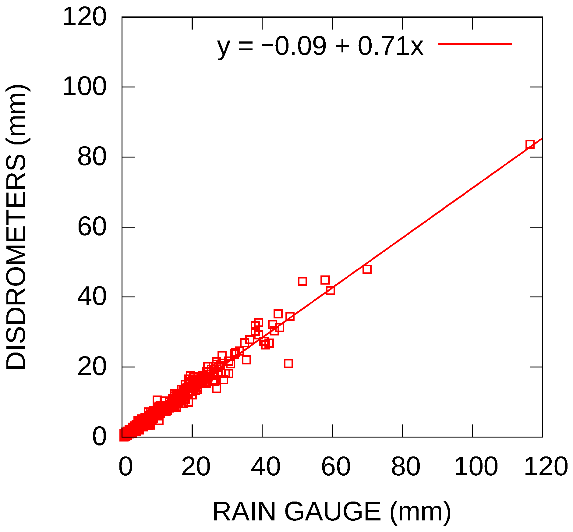
3.1. Comparison with Raingauge

Hourly rainfalls observed while using the disdrometer were compared with the results that were obtained using a collocated tipping-bucket rain gauge (resolution: 0.5 mm) (Figure 2). A total of 959 h of data were utilized, in which at lease one tipping (0.5 mm) was recorded by the rain gauge within 1 h. The selected hourly data also included more than 50 samples of 1-minute disdrometer data with good sensor status (0 or 1), whereas 258-h data were not used because they included more than 10 samples of 1-minute disdrometer data with a bad sensor status (2). The disdrometer systematically underestimated the rainfall amounts by approximately 30%, and the underestimation increased linearly with rainfall intensity.

Figure 3a,b show the daily frequencies of rainfall occurrence and rainfall accumulation, respectively, from 9 May to 31 October 2017, which includes the pre-monsoon, monsoon, and post-monsoon seasons. The accumulated rainfall totals during this period observed by the rain gauge and disdrometer were 9084.5 and 5313.0 mm, respectively. The colour bars presented in Figure 3a,b indicate the rain rates that are based on the disdrometer data; notably, the grey bars presented in Figure 3a indicate periods with a bad sensor status. Rain intensity of <5 mm h${}^{-1}$(>50 mm h${}^{-1}$) occurred during 67% (1%) of the total rainy periods and 17% (15%) of the accumulated rainfall (Figure 3 and

Table 1. Mean drop size distribution (DSD) parameters and integral rain parameters for six rain rate categories.

Category	Num. of 1-min Data	Accum. of Rain	${\mathit{D}}_0$	log${}_{10}{\mathit{N}}_{\mathbf{w}}$	$\mathit{\mu }$	Z	log${}_{10}{\mathit{N}}_{\mathbf{T}}$	log${}_{10}\mathit{LWC}$
$R\ge$80 ${\mathrm{mm} \mathrm{h}}^{-1}$	139 (0.2%)	231.513 mm (4.4%)	2.072	4.162	0.725	51.831	3.581	0.629
50 $\le R<$80 ${\mathrm{mm} \mathrm{h}}^{-1}$	533 (1.1%)	542.623 mm (10.2%)	2.009	4.023	0.974	49.189	3.407	0.421
30 $\le R<$50 ${\mathrm{mm} \mathrm{h}}^{-1}$	1328 (2.7%)	838.700 mm (15.8%)	1.837	4.001	1.874	45.880	3.240	0.232
15 $\le R<$30 ${\mathrm{mm} \mathrm{h}}^{-1}$	3660 (7.4%)	1263.122 mm (23.8%)	1.530	4.158	3.484	41.149	3.140	0.021
5 $\le R<$15 ${\mathrm{mm} \mathrm{h}}^{-1}$	10,578 (21.3%)	1540.990 mm (29.0%)	1.187	4.493	6.508	34.431	3.127	-0.268
$R<$ 5 ${\mathrm{mm} \mathrm{h}}^{-1}$	33,373 (67.3%)	895.592 mm (16.8%)	0.770	4.631	14.759	20.662	2.958	-0.873

).

The transition time between the pre-monsoon season and monsoon season occurs between May and June. Although the frequency of rainfall occurrence and rainfall accumulation are lower before mid-June than during mature monsoon season, the percentage of accumulated intense rainfall with a rate >50 mm h${}^{-1}$ (blue and purple colour bars in Figure 3b) was greater before mid-June than during mature monsoon season. The rain gauge recorded the heaviest daily rainfall (700 mm) on 16 June, whereas the disdrometer recorded a daily rainfall total of 125.5 mm.

July and August constitute the middle of the mature monsoon season and are dominated by intraseasonal variation, with a 10–20-day periodicity, in northeast India [48,49,50]. Three active spells have been identified during July and August in this region: 29 June to 12 July, 18–25 July, and 6–15 August. In 2017, the two active spells in July were relatively weak; however, the active spell in August was relatively strong, with an accumulated rainfall total detected by the rain gauge (the disdrometer) of 1951.5 mm (811.9 mm). Compared with the pre-monsoon season, the rainfall periods during the monsoons were longer, and the contribution of the mid-intensity rain rate (5–30 mm h${}^{-1}$) increased during this time.

Although the monsoon season is over in October, tropical cyclones sometimes affect northeast India. The rainfalls during 19–22 October were affected by a tropical depression, with a maximum surface wind speed between 31 and 50 kmh${}^{-1}$ [51]. This cyclone had formed in the Bay of Bengal on 19 October, landed on the Odisha coast in the afternoon of 20 October, and passed through the south of the Meghalaya Plateau from west to east. The heaviest rainfall was recorded on 21 October, with a daily rainfall amount of 377.5 mm (193.6 mm) by the rain gauge (the disdrometer).

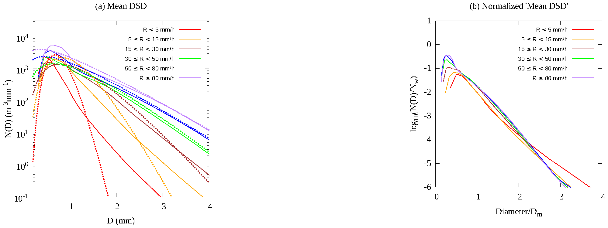
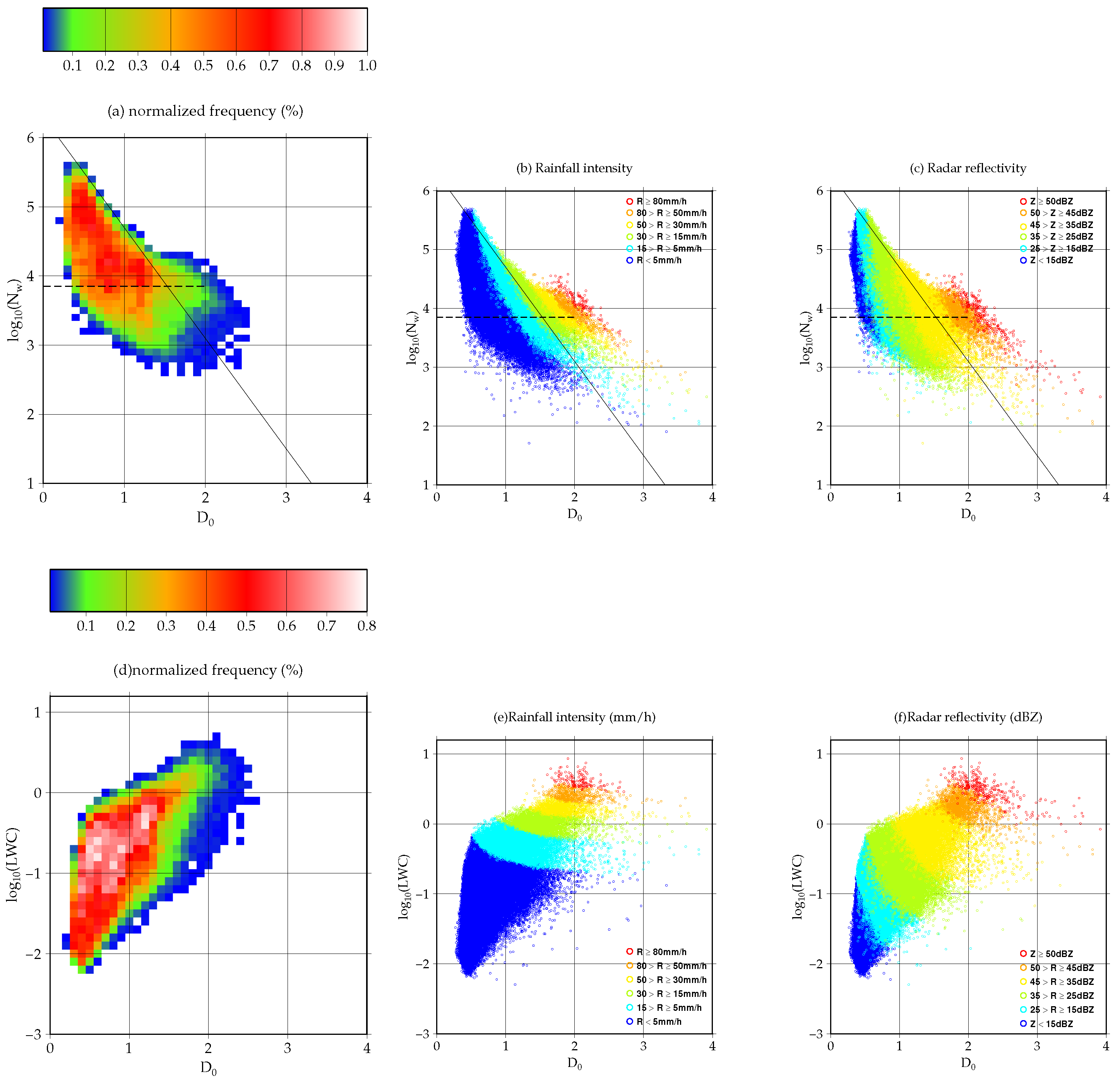
3.2. Features of the DSD

Figure 4a shows the mean DSDs for six rain rate categories (solid lines) and the normalized gamma DSDs while using the mean $N_{\mathrm{w}},D_{\mathrm{m}},\mu$ for the six rain rate categories listed in Table 1 (dashed lines), calculated from 1-min. observation data. The rain rate categories are selected to be consistent with Figure 5b,e, and to be able to focus on intense rain rates. Every peak of the DSD categories was located within a 0–1-mm-diameter range, and the DSDs with intense rain rates have a distinct shoulder-like shape at around 1-mm diameter. As the rain rate became more intense, the DSD included larger raindrops, and the slope parameter of the DSDs decreased, similar to the findings of Marshall and Palmer (1948) [7]. The slope of the mean DSD with a rate of >80 mm h${}^{-1}$ was similar to that of the mean DSD with a rate of 50–80 mm h${}^{-1}$, potentially showing the "number-controlled" condition mentioned by Uijlenhoet et al. (2003) [52]. Friedrich et al. (2016) [53] analyzed the DSDs during the great Colorado flood event and showed a similar result for the DSDs of the intense rain. The DSDs with a rate <5 mm h${}^{-1}$ showed a long tail toward a large D. This is attributable to the composite of a wide range of DSDs, including both LNSD and a smaller number of large drops (Figure 5b). The diameter and $N\left(D\right)$ of Figure 4a are normalized by use of mean values of $D_{\mathrm{m}}$ and $N_{\mathrm{w}}$ (Table 1), respectively, and shown in Figure 4b. The shapes for the categories with more than 15 mm h${}^{-1}$ are very close to one another, and having an exponential form, consistent with the result of Testud et al. (2001).

Table 1 indicates the number and percentage of data in each rain rate category, the DSD parameters, and the rain-integrated parameters. The rainfall with rates of <5 and <15 mm h${}^{-1}$ comprised 67% and 89% of the total rainy periods, respectively. The contribution to the rainfall amount was largest in the 5–30 mm h${}^{-1}$ range and was more than 50% of the total rainfall accumulation. $D_{\mathrm{m}}$, total number concentration $N_{\mathrm{T}}$, radar reflectivity Z, and the $LWC$ increased with the rain rate, whereas the shape parameter $\mu$ became smaller. For all rain rate categories, log${}_{10}{N}_{\mathrm{w}}$ exceeded 4.0.

Figure 5a shows the frequency distribution in the $D_0-{\log }_{10}{N}_{\mathrm{w}}$ space. The solid line in Figure 5a is the stratiform/convective (S/C) separation line proposed by Bringi et al.(2009) [54], and the dashed line corresponds to the S/C line (log${}_{10}{N}_{\mathrm{w}}=3.85$ for tropical maritime precipitation proposed by Thompson et al. (2015) [55]. Figure 5b and c are the same as Figure 5a, except that colour shading is provided to distinguish the six categories in terms of the rain rate and radar reflectivity, respectively. Data with intense rain rates are located in the upper-right of the diagram, and the boundaries between the two categories form curves that correspond to the mathematically derived curves in Rosenfeld and Ulbrich (2003) [3]. The slope of radar reflectivity (Figure 5c) is steeper than that of the rain rate, reflecting the contribution of drop size. The Bringi’s S/C line approximately corresponds to the 15 mm h${}^{-1}$ contour line.

The large number density area of Figure 5a is located on the stratiform side of Bringi’s S/C line and above Thompson’s S/C line, implying the dominance of the LNSD. Bringi et al. (2003) [56] showed the mean stratiform precipitation of various climatic regimes aligned linearly. The mean log${}_{10}{N}_{\mathrm{w}}$ for the rain rate of 5–15 mm h${}^{-1}$ approximately 4.5 (Table 1) in our data, which exceeds the largest mean log${}_{10}{N}_{\mathrm{w}}$ of Papua New Guinea among the different climate regimes. The DSDs with more than 50 mm h${}^{-1}$ have log${}_{10}{N}_{\mathrm{w}}\approx 4.0$ and $D_0\approx 2$ mm (Figure 5b). $D_0\ge 2$ mm is rare in the DSDs of tropical oceanic intense rainfall (Figure 14 of Thompson et al. 2015 [55]). Dolan et al. (2018) [10] compared the $D_0-{\log }_{10}{N}_{\mathrm{w}}$ diagrams for which DSDs were classified by latitude. The shape of the observed distribution resembles that of the mid-latitude more than that of the low latitude and is similar to observations obtained for Beijing, China (Figure 5 of Ji et al. 2019 [57]).

Figure 5d represents the frequency distribution in $D_0-LWC$ space. Figure 5e,f are the same as Figure 5d that colour shading is provided to distinguish the six categories in terms of rain rate and radar reflectivity, respectively. The intense rain rate appears at the top of the distribution, and the contour lines of the rain rates are nearly parallel to the x-axis, reflecting the high correlation between the $LWC$ and rain rate (Figure 5e). The high-frequency area is located at log${}_{10}LWC>-1.2$ and $D_0<1.5$. Rosenfeld and Ulbrich (2003) [3] showed that warm rain over orographic barriers is characterized by a rather small $D_0$ of 0.5–1.0 mm, based on a review of limited studies on orographic rainfall. The results basically agree with those of Rosenfeld and Ulbrich (2003) [3]. In the region of log${}_{10}LWC>0.5$, $D_0$ increased with the $LWC$, rain rate, and Z. This feature is similar to that of tropical maritime warm rain [55]) in that both DSDs tend to have a high $LWC$. However, Cherrapunji DSDs do not have the bimodal distribution observed with tropical maritime rain [55] and, instead, are similar to those at mid-latitudes [10].

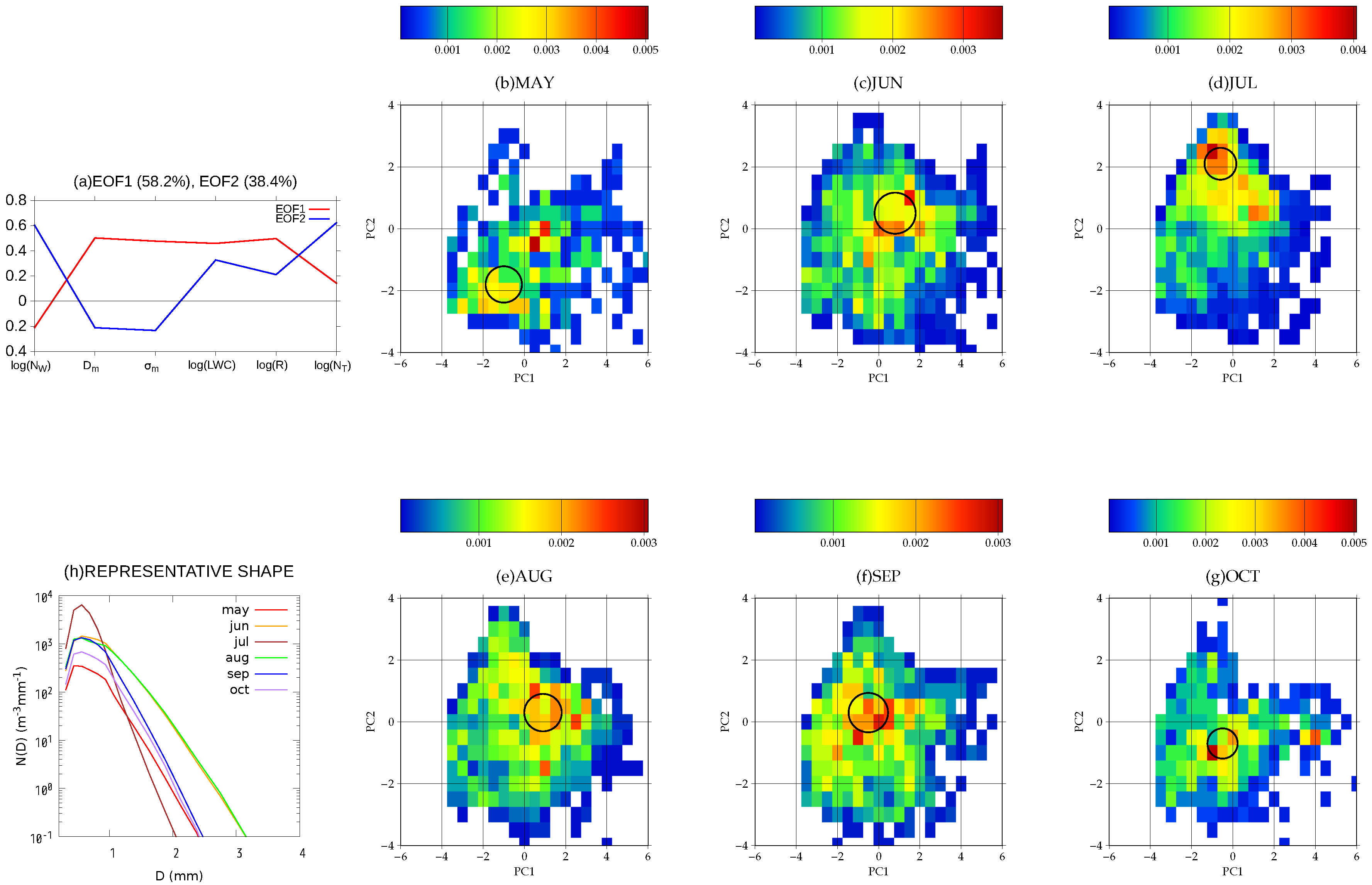
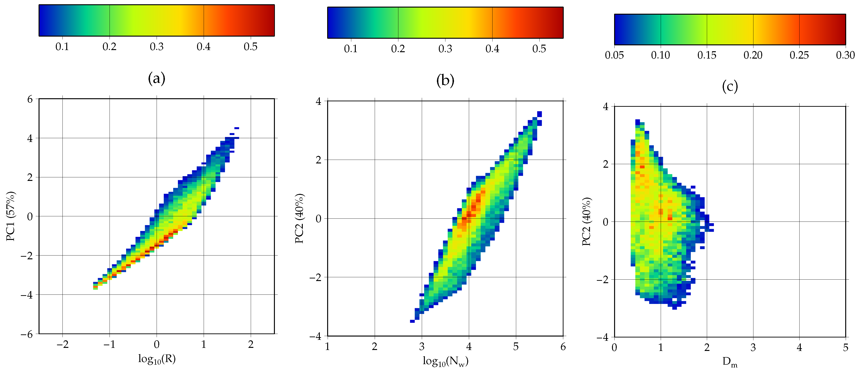
3.3. Seasonal Variation Based on PCA

The first PC of the PCA explains 58.2% of the total variance, whereas the second PC explains 38.4% of the total variance. We neglected the PCs beyond the second PC, which collectively explain a much smaller amount of the variability and may be related to measurement noise of higher-order temporal variability, rather than underlying physical processes. Figure 6a shows the loadings of the first two PCs, represented by EOF1 and EOF2, respectively. The positive mode of EOF1 is associated with a strong positive log${}_{10}LWC$, log${}_{10}R$, $D_{\mathrm{m}}$, and ${\sigma }_{\mathrm{m}}$; a weak positive log${}_{10}{N}_{\mathrm{T}}$; and, weak negative log${}_{10}{N}_{\mathrm{w}}$. The positive mode of EOF2 is characterized by a strong positive log${}_{10}{N}_{\mathrm{w}}$ and log${}_{10}{N}_{\mathrm{T}}$, a weak positive log${}_{10}LWC$, and log${}_{10}R$, and a negative $D_{\mathrm{m}}$ and ${\sigma }_{\mathrm{m}}$. Thus, the LNSD can be expressed by a positive EOF2.

The monthly distributions of the first and second PC scores (represented by PC1 and PC2, respectivey) space are shown in Figure 6b–g. The signs shown in Figure 6b–g correspond to those of Figure 6a. To extract the representative DSDs for each month, a circle was set at an arbitrary point in PC1–PC2 space. The diameter of the circle was determined, such that the circle included 20% of the total number of points for each month. Subsequently, a search was conducted to find the point with the smallest-sized circle. The smallest circles are shown in each figure of Figure 6b–g. Figure 6h shows the representative DSDs averaged over the DSDs inside the circle for each month.

Table 2. Mean DSD parameters and integral rain parameters of the representative DSDs in each month.

Month	${\mathit{D}}_0$	log${}_{10}{\mathit{N}}_{\mathbf{w}}$	$\mathit{\mu }$	Z	log${}_{10}{\mathit{N}}_{\mathbf{T}}$	log${}_{10}\mathit{LWC}$	R
MAY	0.889	3.653	7.912	20.734	2.304	−1.298	0.752
JUN	1.060	4.225	6.114	32.077	2.988	−0.414	6.926
JUL	0.630	5.018	19.630	23.799	3.365	−0.509	3.320
AUG	1.107	4.161	5.578	32.626	2.967	−0.409	7.044
SEP	0.855	4.295	10.068	25.558	2.876	−0.737	2.766
OCT	0.894	3.957	7.427	23.989	2.595	−0.979	1.539

represents the mean parameter values for the representative DSDs for each month.

Clear seasonal differences emerged from the PC-based diagrams (Figure 6b–g). The representative DSDs had a larger PC1 during the monsoon season than pre-monsoon and post-monsoon seasons, reflecting an increase in the rain rates (Table 2). The representative DSDs also had a larger PC2 during the monsoon season than pre-monsoon and post-monsoon seasons, which implies the dominance of the LNSD. Figure 7 shows scatterplots of rain rate vs. PC1, log${}_{10}{N}_{\mathrm{w}}$ vs. PC2, and $D_{\mathrm{m}}$ vs. PC2. The representative DSD in July has the largest PC2, which implies that it includes many LNSD events. The number density distribution in August and September also show a number of LNSD events with a large PC2. The accumulated rainfall in July was less than that in August (Figure 3). Figure 6b–g show that most data with $PC2>2$, corresponding log${}_{10}{N}_{\mathrm{w}}>4.5$ and $D_{\mathrm{m}}<1$ mm (Figure 7) are distributed in the $PC1$ range between −2 and 0, implying a limitation in the rain rate. The increase in the rain rate reduces $N_{\mathrm{w}}$ via the collision–coalescence process.

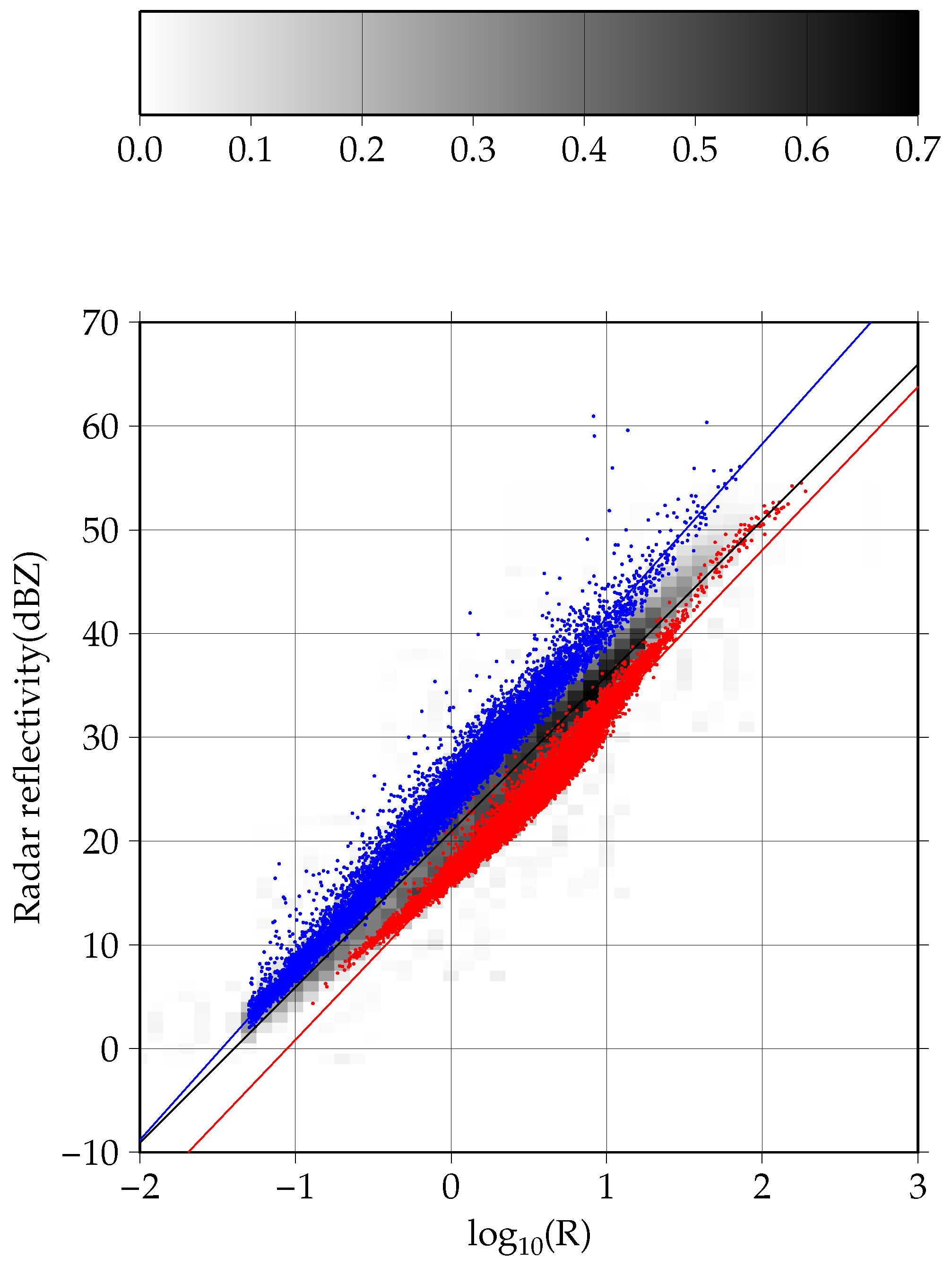
3.4. Contribution of LNSD

In this study, LNSD was defined as samples in which $PC2>+1.5$, based on the PCA described in Section 3.2. For a comparison with the LNSD, the samples with $PC2<-1.5$ are labelled as a small number of drops (SND). Figure 7 shows that the LNSD includes rainfall described by log${}_{10}{N}_{\mathrm{w}}>4.7$ and $D_{\mathrm{m}}<1$ mm, whereas the SND includes rainfall described by log${}_{10}{N}_{\mathrm{w}}<4.0$ and $D_{}>0.5$ mm. Because radar reflectivity Z corresponds to the sixth power of drops, a number of small drops account for the smaller Z and contribute to the smaller estimates of the rain rate R in radar observations. Figure 8 shows a scatter diagram of 1-mm $Z-R$ data, in which the LNSD and SND are shown in red and blue, respectively. The regression line using all samples is given by $Z=124R^{1.50}$. The LNSD is distributed below the regression line, implying a smaller value for parameter A in the $Z=A{R}^b$ relationship. The SND is positioned above the regression line and it includes a wider range for the rain rate. For example, $Z=40$ dBZ corresponds to ≈10 mm h${}^{-1}$ of the SND, while it corresponds to ≈30 mm h${}^{-1}$ of the LNSD.

Figure 9 is the same as Figure 3, except that it represents the contribution of the LNSD and SND to the rainfall occurrence frequency and accumulation. The red, blue, and purple bars represent the rainfalls of LNSD, SND, and others, respectively. The grey bar presented in Figure 9b corresponds to the daily rainfall observed using the rain gauge as a reference. The rainfall occurrence frequency of the SND does not depend on the season, whereas that of the LNSD is clearly dominant during the monsoon period. Especially, the occurrence frequency is high (more than 20% of the active spells from 29 June to 12 July and the beginning of the active spells from 18–25 July and 6–15 August). Figure 9b shows the LNSD produced at approximately 40 and 70 mm for the heavy rainfall days of 2 June and 16 June, respectively. The percentage was the highest on 19 July, at more than 90% of the total rainfall (≈55 mm). However, the percentage of the LNSD was not always high during the active spells. The percentage of the LNSD was small during the latter half of the active spells during 18–25 July and 6–15 August, whereas the contribution of the SND to the accumulated rainfall was small. The contribution of the LNSD to the rainfalls affected by the tropical depression during 19–22 October was rather small, and the LNSD comprised a larger percentage near the end of these rainfall events.

4. Summary and Discussion

Here, we described the observed rain DSD at Cherrapunji, northeast India, where heavy orographic rainfall occurs. The analysis period was from May to October 2017, and the total accumulated rainfall was 5313.0 or 9084.5 mm, as measured by a disdrometer or collocated rain gauge, respectively. The difference in the readings between the disdrometer and rain gauge was due to bad sensor conditions and underestimation of the rainfall by the disdrometer. The comparison of hourly rainfalls showed that the disdrometer 30% underestimated the rainfall amount in comparison with the raingauge (Figure 2). The slopes of the mean DSDs with rain rate of 50–80 mm h${}^{-1}$ and >80 mm h${}^{-1}$ are similar with each other (Figure 4a), and the normalized mean DSD for the categories with more than 15 mm h${}^{-1}$ are very close to one another (Figure 4b). These results imply the DSDs with higher rain rate have equilibrim distribution. The characteristic time to reach equilibrium in coalescence and collisional breakup processes is inversely proportional to the rain rate [58]. Several equilibrium distributions have been proposed [59,60], and all of the shapes have a distinct peak in a 0–1 mm diameter. Though the observed DSDs of higher rain rate in Figure 4a also have a shoulder shape at around 1 mm diameter, the height of peak in a 0–1 mm is relatively low in comparison with the proposed equilibrium distributions. Most disdrometers, including Parsivel${}^2$, have the observation limitation of the small drop size. Recently, Thurai et al. (2017, 2019) [61,62] used a high-resolution (50 microns) meteorological particle spectrometer to capture the small drop end of DSDs (typically diameters $<0.7$ mm) with two-dimensional (2D)-video disdrometer, and showed that the concentration of small drops increase significantly with decreasing drop diameter ($D<0.5$ mm). These past studies imply that the underestimation of the rainfall amount observed by the Parsivel${}^2$ was possibly caused by the improper measurement of small-sized drops. The underestimation in small drops significantly affect the $N_{\mathrm{w}}$ and ${\sigma }_{\mathrm{m}}/D_{\mathrm{m}}$ toward higher values [61].

The $D_0-{\log }_{10}{N}_{\mathrm{w}}$ diagram, which has been used to characterize S/C systems [54] and a variety of different climatic regimes (e.g., [10,55,56,57,63]), was compared with the DSDs that were obtained at other stations. The DSDs were similar to those of tropical oceanic DSDs (e.g., [55]), in that they tended to have a large log${}_{10}{N}_{\mathrm{w}}$; however, the shape of the diagram resembled mid-latitude DSDs [10,57]. The mean log${}_{10}{N}_{\mathrm{w}}$ exceeded 4.0 for all six rain rate categories in the current study; however, the larger $N_{\mathrm{w}}$ was confined to the stratiform side of the S/C separation line that was proposed by Bringi et al. (2009) [54]. The weak updraft along mountainous topography frequently induces shallow warm convection and produces a LNSD. Konwar et al. (2014) [22] conducted aircraft observations over the western Ghats, another orographic heavy rainfall area in India, and reported that the orographically forced updrafts foster rapid condensational growth of cloud droplets triggering coalescence within a few hundred meters of cloud depth. Generally, atmospheric conditions tend to become more unstable over land than over the ocean. The unstable atmosphere can produce buoyancy-generated strong updrafts, thus triggering convection development and cold rain processes in the convection. Lightning observations have indicated a high frequency of flashes over the Meghalaya Plateau [30], implying the existence of cold rain processes, as electrification is associated with supercooled water and graupel [64].

The characteristics of the seasonal variation were analyzed using the PCA approach that was outlined by [10]. The first two principal components explained 96% of the total variance. The first PC had a high positive correlation with rain rate, whereas the second PC had a high positive correlation with $N_{\mathrm{w}}$ and a negative correlation with $D_{\mathrm{m}}$ (Figure 7), implying that positive PC2 can be regarded as a LNSD. Monthly variation was evaluated by the number density distribution in PC1–PC2 space. The representative monthly DSDs were shown by the dense area of the distribution. PC1 increased during the monsoon season, reflecting the dominance of the LNSD. Chakravarty et al. (2003) [26] observed DSDs in Kolkata, India and obtained similar results. The high instability of the atmosphere and the dry conditions in the middle and upper troposphere during the pre-monsoon season [29,65,66] promote strong updraft and evaporation of the rain drops, which can result in an absence of LNSD. In contrast, the atmospheric conditions during the monsoon season are rather stable [67] and wet over the entire troposphere, which can lead to preferential conditions for LNSD development.

The LNSD underestimates radar-derived rainfall by its small radar reflectivity. Rosenfeld and Ulbrich (2003) [3] reviewed past studies and considered that the DSDs of shallow orographic rainfall have a LNSD. Dolan et al. (2018) [10] also regarded LNSD as products from shallow warm convection based on radar observations. Warm convective clouds tend to have a structure that promote a downward increase in the radar reflectivity, regarded as a bottom-heavy precipitation structure (e.g., [6,11,22,68]); this is due to the dominance of the collision-coalescence process, which leads to difficulties in estimating rainfall while using radar due to the ground clutter. The shallowness of the clouds also causes difficulty in detecting precipitation over complicated topographies [12]. Terao et al. (2017) [69] validated the near-surface rain dataset of the Tropical Rainfall Measurement Mission Precipitation Radar (TRMM PR) using tipping-bucket rain gauges over northeast India and Bangladesh; they identified significant underestimation of the TRMM PR near surface rainfall over the Meghalaya Plateau and adjacent Bangladeh plain. The same underestimation was not evident in pre-monsoon data. Their results may be caused by the LNSD.

In this study, the contribution of LNSD to the rainfall at Cherrapunji was defined by $PC2>+1.5$, based on PCA. The LNSD was rare during the pre-monsoon season and dominant in the monsoon season, comprising 16% (19%) of the accumulated rainfall (the total precipitation period). A considerable contribution occurred during the heavy rainfall event on 16 June during a relatively weak active rainfall spell (Figure 9). The LNSD also became dominant at the beginning of the active rainfall spells of the intraseasonal variation during the monsoon season, implying some difficulty in detecting the beginnings of active rainfall periods by remote sensing. The rainfall during 19–22 October was caused by a tropical depression passing through the south of the Meghalaya Plateau from west to east. Although past studies ([20,70] reported the dominance of small- and medium-sized drops during cyclonic rains, the contribution of the LNSD during the passage of the tropical depression was small.

The present study only described the observational results that were obtained from one disdrometer installed at Cherrapunji, northeast India. Future studies are necessary to understand the three-dimensional structure of precipitation systems over the Meghalaya Plateau, using not only disdrometer data, but also ground-based radar and satellite-derived datasets.

References

1. Roe, G.H. Orographic precipitation. Annu. Rev. Earth Planet. Sci. 2005, 33, 645–671. [Google Scholar] [CrossRef]
2. Xie, S.P.; Xu, H.; Saji, N.H.; Wang, Y. Role of narrow mountains in large-scale organization of Asian monsoon convection. J. Clim. 2006, 19, 3420–3429. [Google Scholar] [CrossRef]
3. Rosenfeld, D.; Ulbrich, C.W. Cloud microphysical properties, processes, and rainfall estimation opportunities. in “Radar and Atmospheric Science: A Collection of Essays in Honor of David Atlas”. Meteor. Monogr. 2003, 52, 237–258. [Google Scholar] [CrossRef]
4. Jaffrain, J.; Berne, A. Experimental quantification of the sampling uncertainty associated with measurements from PARSIVEL disdrometers. J. Hydrometeor. 2011, 12, 352–370. [Google Scholar] [CrossRef]
5. Friedrich, K.; Higgins, S.; Masters, F.J.; Lopez, C.R. Articulating and stationary PARSIVEL disdrometer measurements in conditions with strong Winds and heavy rainfall. J. Atmos. Oceanic Technol. 2013, 30, 2063–2080. [Google Scholar] [CrossRef]
6. Zwiebel, J.; Ban Baelen, J.; Anquetin, S.; Pointin, Y.; Boudevillain, B. Impacts of orography and rain intensity on rainfall struction. The case of the HyMeX IOP7a event. Quart. J. Roy. Meteor. Soc. 2016, 142 (Suppl. 1), 310–319. [Google Scholar] [CrossRef]
7. Marshall, J.S.; Palmer, W.M. The distribution of raindrops with size. J. Meteor. 1948, 5, 165–166. [Google Scholar] [CrossRef]
8. Steiner, M.; Smith, J.A.; Uijlenhoet, R. A microphysical interpretation of radar reflectivity-rain rate relationships. J. Atmos. Sci. 2004, 61, 1114–1131. [Google Scholar] [CrossRef]
9. Harikumar, R. Orographic effect on tropical rain physics in the Asian monsoon region. Atmos. Sci. Lett. 2016, 17, 556–563. [Google Scholar] [CrossRef] [Green Version]
10. Dolan, B.; Fuchs, B.; Rutledge, S.A.; Barnes, E.A.; Thompson, E.J. Primary modes of global drop-size distributions. J. Atmos. Sci. 2018, 75, 1453–1476. [Google Scholar] [CrossRef]
11. Liu, C.; Zipser, E.J. Why does radar reflectivity tend to increase downward toward the ocean surface, but decrease downward toward the land surface? J. Geophys. Res. 2013, 118, 135–148. [Google Scholar] [CrossRef] [Green Version]
12. Barros, A.P.; Arulraj, M. Remote sensing of orographic precipitation. In Satellite Precipitation Measurement; Springer: Cham, Switzerland, 2020; Volume 69. [Google Scholar] [CrossRef]
13. Rao, T.N.; Rao, D.N.; Mohan, K. Classification of tropical precipitating systems and associated Z-R relationships. J. Geophys. Res. 2001, 106, 17,699–17,711. [Google Scholar] [CrossRef]
14. Reddy, K.K.; Kozu, T. Measurements of raindrop size distribution over Gadanki during south-west and north-east monsoon. Indian J. Radio Space Phys. 2003, 32, 286–295. [Google Scholar]
15. Sen Roy, S.; Datta, R.K.; Bhatia, R.C.; Sharma, A.K. Drop size distributions of tropical rain over south India. Geofizika 2005, 22, 105–130. [Google Scholar]
16. Harikumar, R.; Kumar, V.S.; Sampath, S.; Vinayak, P.V.S.S.K. Comparison of drop size distribution between stations in eastern and western coasts of India. J. Ind. Geophys. Union 2007, 11, 111–116. [Google Scholar]
17. Kirankumar, N.V.P.; Rao, T.N.; Radhakrishna, B.; Rao, D.N. Statistical characteristics of raindrop size distribution in southwest monsoon season. J. Appl. Meteor. Climatol. 2007, 47, 576–590. [Google Scholar] [CrossRef]
18. Rao, T.N.; Radhakrishna, B.; Nakamura, K.; Rao, N.P. Differences in raindrop size distribution from southwest monsoon to northeast monsoon at Gadanki. Quart. J. Roy. Meteor. Soc. 2009, 135, 1630–1637. [Google Scholar]
19. Sharma, S.; Konwar, M.; Sarma, D.K.; Kalapureddy, M.C.R.; Jain, A.R. Characteristics of rain integral parameters during tropical convective, transition, and stratiform rain at Gadanki and its application in rain retrieval. J. Appl. Meteor. Climatol. 2009, 48, 1245–1266. [Google Scholar] [CrossRef] [Green Version]
20. Kumar, S.B.; Reddy, K.K. Rain drop size distribution characteristics of cyclonic and north east monsoon thunderstorm precipitating clouds observed over Kadapa (14.47° N, 78.82° E), tropical semi-arid region of India. Mausam 2013, 64, 35–48. [Google Scholar]
21. Sulochana, Y.; Rao, T.N.; Sunilkumar, K.; Chandrika, P.; Raman, M.R.; Rao, S.V.B. On the seasonal variability of raindrop size distribution and associated variations in reflectivity - rainrate relations at Trupati, a tropical station. J. Atmos. Solar-Terrestorial Phys. 2016, 147, 98–105. [Google Scholar] [CrossRef]
22. Konwar, M.; Das, S.K.; Deshpande, S.M.; Chakravarty, K.; Goswami, B.N. Microphysics of clouds and rain over the Western Ghat. J. Geophys. Res. 2014, 119, 6140–6159. [Google Scholar] [CrossRef]
23. Deshpande, S.M.; Dhangar, N.; Das, S.K.; Kalapureddy, M.C.R.; Chakravarty, K.; Sonbawne, S.; Konwar, M. Mesoscale kinematics derived from X-band Doppler radar observations of convective versus stratiform precipitation and comparison with GPS radiosonde profiles. J. Geophys. Res. 2015, 120, 11536–11551. [Google Scholar] [CrossRef]
24. Utsav, B.; Deshpande, S.M.; Das, S.K.; Pandithurai, G. Statistical characteristcis of convective clouds over the Western Ghats derived from westhern radar observations. J. Geophys. Res. 2017, 122, 10050–10076. [Google Scholar] [CrossRef]
25. Utsav, B.; Deshpande, S.M.; Das, S.K.; Pandithurai, G.; Niyogi, D. Observed vertical structure of convection during dry and wet summer monsoon epochs over the Western Ghats. J. Geophys. Res. 2019, 124, 1352–1369. [Google Scholar] [CrossRef]
26. Chakravarty, K.; Raj, P.; Bhattacharya, A.; Maitra, A. Microphysical characteristics of clouds and precipitation during pre-monsoon and monsoon period over a tropical Indian station. J. Atmos. Solar-Terrestorial Phys. 2013, 94, 28–33. [Google Scholar] [CrossRef]
27. Stiller-Reeve, M.A.; Syed, M.A.; Spengler, T.; Spinney, J.A.; Hossain, R. Complementing scientific monsoon definitions with social perception in Bangladesh. Bull. Amer. Meteor. Soc. 2015, 96, 49–57. [Google Scholar] [CrossRef] [Green Version]
28. Zipser, E.J.; Cecil, D.J.; Liu, C.; Nesbitt, S.W.; Yorty, D.P. Where are the most intense thunderstorms on earth? Bull. Amer. Meteor. Soc. 2006, 96, 1057–1071. [Google Scholar] [CrossRef] [Green Version]
29. Das, S.; Mohanty, U.C.; Tyagi, A.; Sikka, D.R.; Joseph, P.V.; Rathore, L.S.; Habib, A.; Baidya, S.K.; Sonam, K.; Sarkar, A. The SAARC STORM: A coordinated field experiment on severe thunderstorm observations and regional modeling over the South Asian region. Bull. Amer. Meteor. Soc. 2014, 95, 603–617. [Google Scholar] [CrossRef] [Green Version]
30. Choudhury, B.A.; Konwar, M.; Hazra, A.; Mohan, G.M.; Pithani, P.; Ghude, S.D.; Deshamukhya, A. A diagnostic study of cloud physics and lightning flash rates in a severe pre-monsoon thunderstorm over northeast India. Quart. J. Roy. Meteor. Soc. 2020, 1–22. [Google Scholar] [CrossRef]
31. Loffler-Mang, M.; Joss, J. An optical disdrometer for measuring size and velocity of hydrometers. J. Atmos. Oceanic Technol. 2000, 17, 130–139. [Google Scholar] [CrossRef]
32. Loffler-Mang, M.; Blahak, U. Estimation of the equivalent radar reflectivity factor from measured snow size spectra. J. Appl. Meteor. 2001, 40, 843–849. [Google Scholar] [CrossRef]
33. Battaglia, A.; Rustemier, E.; Tokay, A.; Blahak, U.; Simmer, C. PARSIVEL snow observations: A critical assessment. J. Atmos. Oceanic Technol. 2010, 27, 333–344. [Google Scholar] [CrossRef]
34. Tokay, A.; Petersen, W.A.; Gatlin, P.; Wingo, M. Comparison of raindrop size distribution measurements by collocated disdrometers. J. Atmos. Oceanic Technol. 2013, 30, 1672–1690. [Google Scholar] [CrossRef]
35. Tokay, A.; Wolff, D.B.; Petersen, W.A. Evaluation of the new version of the laser-optical disdrometer, OTT Parsivel2. J. Atmos. Oceanic Technol. 2014, 31, 1276–1288. [Google Scholar] [CrossRef]
36. Angulo-Martinez, M.; Begueria, S.; Latorre, B.; Fernandez-Raga, M. Comparison of precipitation measurements by OTT Parsivel2 and Thies LPM optical disdrometers. Hydrol. Earth Syst. Sci 2018, 22, 2811–2837. [Google Scholar] [CrossRef] [Green Version]
37. Kalina, E.A.; Friedrich, K.; Ellis, S.M.; Burgess, D.W. Comparison of disdrometer and X-band mobile radar observations in convective precipitation. Mon. Wea. Rev. 2014, 142, 2414–2435. [Google Scholar] [CrossRef] [Green Version]
38. Gunn, R.; Kinzer, G.D. The terminal velocity of fall for water droplets in stagnant air. J. Meteor. 1949, 6, 243–248. [Google Scholar] [CrossRef] [Green Version]
39. Atlas, D.; Srivastava, R.C.; Sekhon, R.S. Doppler radar characteristics of precipitation at vertical incidence. Rev. Geophys. 1973, 11, 1–35. [Google Scholar] [CrossRef]
40. Smith, P.L.; Liu, Z.; Joss, J. A study of sampling-variability effects in raindrop size observations. J. Appl. Meteor. 1993, 32, 1259–1269. [Google Scholar] [CrossRef] [Green Version]
41. Smith, P.L. Sampling issues in estimating radar variables from disdrometer data. J. Atmos. Oceanic Technol. 2016, 33, 2305–2313. [Google Scholar] [CrossRef]
42. Willis, P.T. Functional fits to some observed drop size distributions and parameterization of rain. J. Atmos. Sci. 1984, 41, 1648–1661. [Google Scholar] [CrossRef] [Green Version]
43. Testud, J.; Oury, S.; Black, R.A.; Amayenc, P.; Dou, X. The concept of “normalized” distribution to describe raindrop spectra: A tool for cloud physics and cloud remote sensing. J. Appl. Meteor. 2001, 40, 1118–1140. [Google Scholar] [CrossRef]
44. Bringi, V.N.; Huang, G.J.; Chandrasekar, V. A methodology for the parameters of a gamma raindrop size distribution model from polarimetric radar data: Application to a squall-line event from the TRMM/Brazil campaign. J. Atmos. Oceanic Technol. 2002, 19, 633–645. [Google Scholar] [CrossRef] [Green Version]
45. Ulbrich, C.W. Natural variations in the analytical form of the raindrop size distribution. J. Appl. Meteor. 1983, 22, 1764–1775. [Google Scholar] [CrossRef] [Green Version]
46. Cao, Q.; Zhang, G. Errors in estimating raindrop size distribution parameters employing disdrometer and simulated raindrop spectra. J. Appl. Meteor. Climatol. 2009, 48, 406–425. [Google Scholar] [CrossRef]
47. Williams, C.R.; Bringi, V.N.; Carey, L.D.; Chandrasekar, V.; Gatlin, P.N.; Haddad, Z.S.; Meneghini, R.; Munchak, S.J.; Nesbitt, S.W.; Petersen, W.A.; et al. Describing the shape of raindrop size distributions using uncorrelated raindrop mass spectrum parameters. J. Appl. Meteor. Climatol. 2014, 53, 1282–1296. [Google Scholar] [CrossRef]
48. Fujinami, H.; Hatsuzuka, D.; Yasunari, T.; Terao, T.H.T.; Murata, F.; Kiguchi, M.; Yamane, Y.; Matsumoto, J.; Islam, M.N.; Habib, A. Characteristic intraseasonal oscillation of rainfall and its effect on interannual variability over Bangladesh during boreal summer. Int. J. Climatol. 2011, 31, 1192–1204. [Google Scholar] [CrossRef]
49. Fujinami, H.; Sato, T.; Kanamori, H.; Murata, F. Contrasting Features of Monsoon Precipitation Around the Meghalaya Plateau Under Westerly and Easterly Regimes. J. Geophys. Res. 2017, 122. [Google Scholar] [CrossRef]
50. Murata, F.; Terao, T.; Fujinami, H.; Hayashi, T.; Asada, H.; Matsumoto, J.; Syiemlieh, H.J. Dominant synoptic disturbance in the extreme rainfall at Cherrapunji, northeast India, based on 104 years of rainfall data (1902–2005). J. Climate 2017, 30, 8237–8251. [Google Scholar] [CrossRef]
51. India Meteorological Department. Depression over westcentral Bay of Bengal (19–22 October, 2017): A Report. Available online: http://rsmcnewdelhi.imd.gov.in/images/pdf/publications/preliminary-report/d19-22oct.pdf (accessed on 16 July 2020).
52. Uijlenhoet, R.; Smith, J.A.; Steiner, M. The microphysical structure of extreme precipitation as inferred from ground-based raindrop spectra. J. Atmos. Sci. 2003, 60, 1220–1238. [Google Scholar] [CrossRef]
53. Friedrich, K.; Kalina, E.A.; Aikins, J.; Steiner, M.; Gochis, D.; Kucera, P.A.; Ikeda, K.; Sun, J. Raindrop size distribution and rain characteristics during the 2013 great Colorado flood. J. Hydrometeor. 2016, 17, 53–72. [Google Scholar] [CrossRef]
54. Bringi, V.N.; Williams, C.R.; Thurai, M.; May, P.T. Using dual-polarized radar and dual-frequency profiler for DSD characterrization: A case study from Darwin, Australia. J. Atmos. Oceanic Technol. 2009, 26, 2107–2122. [Google Scholar] [CrossRef]
55. Thompson, E.J.; Rutledge, S.A.; Dolan, B. Drop size distributions and radar observations of convective and stratiform rain over the equatorial Indian and west Pacific Oceans. J. Atmos. Sci. 2015, 72, 4091–4125. [Google Scholar] [CrossRef]
56. Bringi, V.N.; Chandrasekar, V.; Hubbert, J. Raindrop size distribution in different climatic regimes from disdrometer and dual-polarized radar analysis. J. Atmos. Sci. 2003, 60, 354–365. [Google Scholar] [CrossRef]
57. Ji, L.; Chen, H.; Li, L.; Chen, B.; Xiao, X.; Chen, M.; Zhang, G. Raindrop size distributions and rain characteristics observed by a PARSIVEL disdrometer in Beijing, northern China. Remote Sens. 2019, 11, 1479. [Google Scholar] [CrossRef] [Green Version]
58. Srivastava, R.C. On the scaling of equations governing the evolution of raindrop size distributions. J. Atmos. Sci. 1988, 45, 1091–1092. [Google Scholar] [CrossRef] [Green Version]
59. McFarquhar, G.M. A new representation of collision-induced breakup of raindrops and its implications for the shapes of raindrop size distributions. J. Atmos. Sci. 2004, 61, 777–794. [Google Scholar] [CrossRef] [Green Version]
60. Straub, W.; Beheng, K.D.; Seifert, A.; Schlottke, J.; Weigand, B. Numerical investigation of collision-induced breakup of raindrops. Part II: Parameterizations of coalescence efficiencies and fragment size distributions. J. Atmos. Sci. 2010, 67, 576–588. [Google Scholar] [CrossRef] [Green Version]
61. Thurai, M.; Gatlin, P.; Bringi, V.N.; Petersen, W.; Kennedy, P.; Notaros, B.; Carey, L. Toward completing the raindrop size spectrum: Case studies involving 2D-video disdrometer, droplet spectrometer, and polarimetric radar measurements. J. Atmos. Oceanic Technol. 2017, 56, 877–896. [Google Scholar] [CrossRef]
62. Thurai, M.; Bringi, V.; Gatlin, P.N.; Petersen, W.A.; Wingo, M.T. Measurements and modeling of the full rain drop size distribution. Atmosphere 2019, 10, 39. [Google Scholar] [CrossRef] [Green Version]
63. Marzuki, M.; Hashiguchi, H.; Yamamoto, M.K.; Mori, S.; Yamanaka, M.D. Regional variability of raindrop size distribution over Indonesia. Ann. Geophys. 2013, 31, 1941–1948. [Google Scholar] [CrossRef] [Green Version]
64. Houze, R.A. Cloud Dynamics; Academic Press: Oxford, UK, 2014. [Google Scholar]
65. Yamane, Y.; Hayashi, T.; Dewan, A.M.; Akter, F. Severe local convective storms in Bangladesh: Part II. Environmental conditions. Atmos. Res. 2010, 95, 407–418. [Google Scholar] [CrossRef]
66. Murata, F.; Terao, T.; Kiguchi, M.; Fukushima, A.; Takahashi, K.; Hayashi, T.; Habib, A.; Bhuiyan, M.S.H.; Choudhury, S.A. Daytime thermodynamic and airflow structures over northeast Bangladsh during the pre-monsoon season: A case study on 25 April 2010. J. Meteor. Soc. Japan 2011, 89A, 167–179. [Google Scholar] [CrossRef] [Green Version]
67. Yamane, Y.; Hayashi, T. Evaluation of environmental conditions for the formation of severe local storms across the Indian subcontinent. Geophys. Res. Lett. 2006, 33. [Google Scholar] [CrossRef]
68. Wilson, A.M.; Barros, A.P. An investigation of warm rainfall microphysics in the southern Appalachians: Orographic enhancement via low-level seeder-feeder interactions. J. Atmos. Sci. 2014, 71, 1783–1805. [Google Scholar] [CrossRef]
69. Terao, T.; Murata, F.; Yamane, Y.; Kiguchi, M.; Fukushima, A.; Tanoue, M.; Ahmed, S.; Choudhury, S.A.; Syiemlieh, H.J.; Cajee, L.; et al. Direct validation of TRMM/PR near surface rain over the northeastern Indian subcontinent using a tipping bucket raingauge network. SOLA 2017, 13, 157–162. [Google Scholar] [CrossRef]
70. Radhakrishna, B.; Rao, T.N. Differences in cyclonic raindrop size distribution from southwest to northeast monsoon season and from that of noncyclonic rain. J. Geophys. Res. 2010, 115. [Google Scholar] [CrossRef]
Figure 1. Topography over northeast India (unit: m) and location of Cherrapunji town (91.72 E, 25.27 N, 1313 m MSL) indicated by a star.
Atmosphere 11 00777 g001
Figure 2. Comparison of hourly rainfalls between Parsivel 2 and tipping-bucket raingauge. The total number of samples is 959, which at least one tipping (0.5 mm) was recorded by the rain gauge, and data also includes more than 50 one-minute samples with good sensor status (0 or 1).
Atmosphere 11 00777 g002
Figure 3. (a) The frequency of occurrence in daily rainfall, and (b) the accumulated rainfall fraction during May–October 2017. The gray bars in (a) indicate the periods of no data due to bad sensor status, and the gray bars in (b) indicate daily rainfall amount observed in the collocated raingauge. Note that the raingauge had stopped during 1–3 July.
Atmosphere 11 00777 g003
Figure 4. (a) Mean DSDs for six rain rates categories: less than 5 mm h 1 (red solid line), 5 R < 15 mm   h 1 (orange), 15 R < 30 mm   h 1 (brown), 30 R < 50 mm   h 1 (green), 50 R < 80 mm   h 1 (blue), and R 80 mm   h 1 (purple), respectively. The dotted lines are the estimated gamma distributions that are based on the mean DSD parameters ( D m , N w , μ ) of each rain rate category listed in Table 1. (b) Normalized ’mean DSDs’ by use of N w and D m .The meaning of the colored solid lines is same as (a).
Atmosphere 11 00777 g004
Figure 5. (a)–(c) D 0 log 10 N w and (d)–(f) D 0 log 10 L W C diagrams. (a,d) The number density (%), (b,e) the distribution of six categories of rain rates, and (c,f) the distribution of the six categories of radar reflectivities are shown. Solid and dashed lines in (a)–(c) are the stratiform/convective separation lines proposed by Bringi et al. [54] and Thompson et al. [55], respectively.
Atmosphere 11 00777 g005
Figure 6. (a) The loadings of the first two PCs, represented by EOF1 and EOF2, respectively. (b)–(g) Monthly distributions of the first and second component scores (represented by PC1 and PC2, respectively) space for (b) May, (c) June, (d) July, (e) August, (f) September, and (g) October. The circles in each figure show the minimum circle that includes 20% of the total samples in each month. (h) The mean DSDs of the samples included within the circles in (b)–(g).
Atmosphere 11 00777 g006
Figure 7. Number density (%) in the (a) log 10 R -PC1, (b) log 10 N w -PC2, and (c) D m -PC2 spaces.
Atmosphere 11 00777 g007
Figure 8. Relationship between radar reflectivity Z ( dBZ ) and rain rate R ( mm   h 1 ). Solid black line is the regression line represented by Z ( mm 6 m 3 ) = 124 R 1.50 ( mm   h 1 ) . The red and blue points are the data of P C 2 > + 1.5 and P C 2 < 1.5 , respectively. The solid red and blue lines are the regression lines of the red and blue points, respectively.
Atmosphere 11 00777 g008
Figure 9. (a) The frequency of occurrence in daily rainfall, and (b) the accumulated rainfall fractions with P C 2 > + 1.5 (red color) and P C 2 < 1.5 (blue color), and others (purple color) during 1 May–31 October 2017. The gray bars in (a) indicate the periods of missing data due to bad sensor status, and the gray bars in (b) indicate the accumulated rainfall observed by the collocated raingauge.
Atmosphere 11 00777 g009