Estimation of Damage Cost to Building Façades per kilo Emission of Air Pollution in Norway

Abstract

This work reports marginal damage costs to façades due to air pollution exposure estimated “bottom up,” for Norway and Oslo (Norway) by the use of exposure response functions (ERFs) and impact pathway analysis from the emission to the deteriorating impact. The aim of the work was to supply cost estimates that could be compared with reported damage costs to health, agriculture, and ecosystems, and that could be used in cost-benefit analysis by environmental authorities. The marginal damage costs for cleaning, repair, and in total (cleaning + repair) were found to be, in Norway: eight, two, and 10, respectively, and for a traffic situation in Oslo: 50 (77), 50 (28), and 100 (105), (×/÷ 2.5) Euro/kg emission of PM₁₀, SO₂, and NO₂ in total. For Oslo, the values represent a recorded façade materials inventory for 17–18th century buildings, and in the brackets the same façade inventory as for Norway. In total, 5–10% of the marginal damage cost was found to be due to NO₂. The total marginal cost was found to be shared about equally between the impact of PM₁₀ and SO₂ in Norway (50 and 42% of the impact) and for the 17–18th century buildings in Oslo (45% and 49% of the impact), but for a similar façade materials inventory in Oslo as Norway, the total marginal cost due to PM₁₀ was about two-thirds and that due to SO₂ about one-third of the total, with about 5% of the cost still being due to NO₂. The division of the costs between the separate pollutant influences on the cleaning and repair was, however, found to be significantly different in Norway and Oslo. In Norway, about 60% of the marginal cleaning cost was found to be due to PM₁₀, 30% due to SO₂, and 10% due to NO₂. In Oslo, about 85% of the marginal cleaning costs were found to be due to PM₁₀, 10% due to SO₂, and 5% due to NO₂. For the marginal repair cost, the opposite situation was found, in both Norway and Oslo, with 80–90% of the cost being due to SO₂, 5–10% being due to PM₁₀, and 5–10% due to NO₂. As other factors than air pollution deteriorates façades and influences maintenance decisions, the expenses that can be attributed to the air pollution could be significantly lower.

1. Introduction

In this work, the marginal damage costs to building façades per kilo emission of air pollution were estimated “bottom up” by impact pathway analysis (IPA) from the pollution emissions to the effect, for a regional Norwegian and urban scenario in Oslo, Norway, by the Uniform World Model method described by [1], and using damage functions (exposure-response functions, ERFs) for the pollution influence on the façade materials developed through [2] (ICP materials, the International Co-operative Programme on Effects on Materials including Historic and Cultural Monuments, within the Convention on Long-range Transboundary Air Pollution, CLRTAP). The purpose of the work was to supply cost estimates to environmental authorities that could be compared with reported damage costs to health, agriculture, and ecosystems, and that can be used in cost-benefit analysis. Few cases of air pollution cost analysis for buildings have been reported in the scientific literature, the cost units have been many and hard to compare [3], and the marginal costs per emission, most useful for policy makers, have seldom been reported.

Air pollution is a consequence of our economic activities. It damages people’s health [4,5,6], reduces crops, has negative impacts on vegetation and ecosystems [7,8,9] and damages the built environment [10,11], with consequent costs to society. The environmental costs have been described as “external” to the decision makers’ main, often short term, economic goals. As such, they have often not been fully included in accounting. The costs then cannot be fully assessed by the expenses for the “repair,” and the expenses that appear in budgets are likely to be less than the costs to society. The long-term consequence of such omission is non-sustainability and reduced welfare. Externality costs, including those due to air pollution, should be estimated and reported, to allow cost-benefit analysis that can include the negative impacts. Decisions based on well informed cost-benefit analysis will, ideally, assure that the preferred outcomes are reached, which provide the highest benefit at the lowest costs. The valuation of costs and benefits and thus the outcomes, may involve judgements about preferences and the distribution of the benefits, which are political in nature.

The air pollution cost to health have been found to contribute by far the largest part of the quantified damage costs due to air pollution [1], and are thus considered the most serious. Air pollution aggravates morbidity, especially due to respiratory and cardiovascular diseases, and leads to premature mortality [1,5]. Many estimates exist of the loss of quality of life and life expectancy due to air pollution, but relatively few estimates of the cost to the built environment have been reported. The health related costs in Europe in the year 2000 were reported to be in the range from about 20 to 45 Euro per kg emission of PM_2.5 (particles with an aerodynamic diameter less than 2.5 µm) depending on stack height, about 10 Euro per kg SO₂, and about 6 Euro per kg NO₂ [1] (p. 504–509). About similar damage cost as to health by exposure to PM₁₀ emitted as non-combustion road dust have been reported for Sweden in 2016 due to soiling of façades per kilo total emitted PM₁₀, of about 1–6 Euro in villages and small towns, up to 60–80 Euro in large towns [12] (p. 91). These values were reworked in a later report to give values in Sweden, now also including discounting of the cost by 14% over an assumed period of 10 years between renovation action and including a doubling of the costs due to amenity loss of appearance, ranging from 10 Euro per kg PM₁₀ in small towns to up to 50 Euro per kg in Stockholm, with a recommended value to apply in societal cost analysis of emission from the transport sector causing soiling in cultural environments, of 32 Euro per kg [13].

As compared to these damage costs to health and the soiling cost reported for Sweden, the marginal damage costs to building materials from exposure to each kg emitted SO₂ in Norway in the 1990s were reported to be 0.3–13 Euro in the major cities (11 Euro in Oslo), 0.1–0.3 Euro in other towns and villages with more than 15,000 people, and about 0.01 Euro in the remaining regions [14]. For Europe, the typical marginal damage cost due to SO₂ has been reported to be from 0.1 to 0.4 Euro per kg, representing 1–4% of the health costs [1] (p. 131). The renovation expenses of façades in France in 1994 that were explained by exposure to PM₁₀ were reported to probably be in the range from 0.07 to 0.3 Euro per kg [1] (p. 156). For the particle exposure, the costs were reported to represent a regional and middle-income situation and included a doubling of the cost due to amenity loss. The results for Sweden in 2016 and Norway in the 1990s were obtained with exposure-response modelling, as applied in this work, whereas the soiling costs for France were obtained from deductions of building renovation expenditures correlated with measured PM concentrations. In this instance, for France, it was reported that for transport emissions in cities, the cost would be higher [1] (p. 156): as the reported marginal costs “has to be multiplied with the correction factors of the UWM” (Uniform World Model, see Method section). The higher urban than rural (background) costs, due to local air pollution, emphasizes the anthropogenic factors driving the cost development and the possibility for mitigation policies to reduce costs.

Results from “top-down” studies can be used to validate results calculated bottom-up, but there are considerable uncertainty and possible biases with both methods that need to be considered. The uncertainty in “bottom-up” estimations is related to the representation of complex façade deterioration by the ERFs and in the emissions-to-exposure assessment by the UWM in this case. The available ERFs were developed by the exposure of small samples of a selection of standard experimental materials in a situation with a changing environment, with historically much more SO₂, and changing building technology. The degradation and maintenance of façades happens, partly, by other mechanisms and for other reasons than the uniform atmospheric wear, as measured in experiments. These influences may not simply add to the effect of the air pollution, but more or less substitute it. It can be physical impacts, such as with water penetration, salt crystallization and dissolution, freeze thaw cycles and thermoclastism [15], and related dimensional changes, which can also interact with air pollution in different ways. Aesthetical and budgetary concerns can be important. In “top-down” studies, it can be difficult to assure complete records for the renovation expenses and the factors that influence the spending. In addition, externality cost will not be included in budgets.

Thus, the marginal costs and expenses due to the air pollution may be some fraction of that when the atmospheric wear is the only reason for the maintenance [16]. The magnitude of this fraction could be evaluated from the total conditions for the façade and maintenance, besides the assessment of the pollution effect.

To obtain and report the range of the most probable values for the marginal costs, it seems essential to discuss the uncertainties and possible biases. This is needed when the results from the bottom-up and top-down studies are compared, for validation.

The terms “effect,” “influence,” and “impact” are used interchangeably in this work, but “effect” usually in the more technical descriptions of the calculations, and “influence” and “impact” more generally. The maintenance of façades will often be both by cleaning, and by renovation involving different kinds of repair, such as repainting or replacement. The term “repair” will be used loosely to represent all kinds of maintenance operations on façades, except cleaning. The term “maintenance” will include cleaning. As there is considerable uncertainty in calculations of marginal damage costs of façades due to air pollution, it was an aim to do the cost calculations as efficiently as possible without introducing more ERFs or categories of façade materials than would improve the result. The calculations in this work are based on the assumption that façades are renovated regularly at frequencies corresponding to the “lifetime between maintenance.” When the façades have deteriorated to a recordable reduced condition, renovation of the previous condition then takes place by some renovation action for which the price is known.

The scenarios are described in the Methods section and will throughout the paper mostly be termed simply “Norway” and “Oslo.” The Oslo scenario represents one well documented urban traffic case. In the Discussion section, a comparison between Norway and Oslo is also made using “the Norway façades inventory” for Oslo. It is left to the reader to remember that these are scenarios designed to resemble Norway regionally and an urban area of Oslo, but they do not claim to represent the actual situation in Norway and Oslo.

This work was to a large extent based on the methods described by [1], and therefore, includes many references to their work. The parameters and units used in this work, except the notations for different types of façade materials in

Table 1. Equations, broken up in 10 terms.

	Marginal Cost, Dtot =	Façade Material, i.
1.	[(1 − Fr − Fw) × DP,fc]	fc = general façades, cleaning
2.	+ [Fw × (DS,wc + DN,wc + DP,wc)]	wc = window glass, cleaning
3.	+ [Fr × (DS,r + DN,r + DP,r)]	r = renderings
4.	+ [Fl × (DS,l + DN,l + DP,l)]	l = limestone
5.	+ [Fps × DS,ps]	ps = painted steel
6	+ [Fpom × DS,pom]	pom = painted materials other than steel
7.	+ [Fpw × DS,pw]	pw = painted wood
8.	+ [Fc × DS,c]	c = copper
9.	+ [Fz × DS,z]	z = zinc including galvanizing
10.	+ [Fb × DS,b]	b = brick, tile and concrete

, are given in

Table A1. Parameters and units.

Parameter	Explanation	Unit
A	Urban conurbation area	m2
DR	Dilution rate for a ground level sources	m2/s
${\dot{D}}_{UWM,p,i}$	Damage cost rate on material, i, due to pollutant, p	Euro/year
${\dot{D}}_{UWM,p,i}^{ground}$	Damage cost rate of ground level sources in cities	Euro/year
Dp,i	Marginal damage cost on material, i, due to pollutant, p	Euro/kg
Dtot	Marginal damage cost on the façade inventory	Euro/kg
fec	Empirical correction factor for cleaning responses	fraction
Fi	Fraction of façade material, i, to the total façade area	m2/m2
funi	Background façade density	m2 material area/m2 ground area
H	Haze	%
H+	Concentration of H+ ions (acidity, pH) in precipitation	mg/L
[HNO3]	Nitic acid concentration in air	µg/m3
k	Deposition velocity	cm/s
LFD	Linear façade density	m2 façade area/m
${\dot{\mathrm{m}}}_{\mathrm{p}}$	Emission rate	kg/year
ML	Mass loss	g/m2
N	Number of receptors, i.e., façade square meters	m2
[NO2]	Nitrogen dioxide concentration in air	µg/m3
[O3]	Ozone concentration in air	µg/m3
p	Pollution species
pH	Acidity
Pi	Renovation price for material, i
[PM10]	Concentration in air of particle matter with aerodynamic diameter < 10 µm	µg/m3
[PM13]	Concentration in air of particle matter with aerodynamic diameter < 13 µm	µg/m3
R	Deterioration response	%, g/m2 or µm
R2	Explanatory power of equation
R0	Reflectance of a non-soiled surface	%
∆R	Loss of reflectance	%
Rain	Annual precipitation amount	mm
Rh	Relative humidity	%
Rh60	(Rh-60) when Rh > 60, otherwise 0	%
Seg	Adjustment factor for ground level sources
SERF,p,i	Slope of the exposure response functions for pollutant, p, and material, i	1/year × µg/m3
[SO2]	Sulfur dioxide concentration in air	µg/m3
T	Temperature	°C
t	Time	years or days
tinitial	Time before cracking of paint	years

.

2. Method

2.1. Exposure-Response Functions and Marginal Maintenance Cost Estimations

The damage costs per kilo emission of air pollution that causes atmospheric wear of building façades in Norway and the city of Oslo, Norway, were calculated “bottom up” from the averaged exposure and maintenance conditions. The considered atmospheric wear was soiling causing a need for cleaning and atmospheric chemical wear, often termed corrosion, causing a need for maintenance. The costs were calculated by the multiplication of a physical deterioration measure, the response, with a value for the maintenance price. They do not consider the time evolution of costs in terms of discounting or interest rates.

Available published exposure response functions (ERFs) (see Appendix A) were used to calculate the impact of the air pollution on each façade material. The ERFs were developed from experimental exposures of sample materials, generally of a dimension of 10 cm × 15 cm, which could represent façades. The exposures were carried out on 57 different stations (52 in Europe, four in North America, and one in Israel) over the years of the ICP materials project since 1987, changing from 39 stations in 1987 to 24 stations in 2017 [2]. Applying ERFs from laboratory-scale samples for the assessment of full-scale façades is challenging due to complex geometries, dissimilar materials interactions, and mechanical loading absent during testing. It is the “atmospheric wear” of façades as represented by experimental samples, which is estimated in this work.

The simplified Uniform World Model (UWM) [1] was used to estimate the marginal damage cost, as Euro per kilo pollutant uniformly dispersed from the emission source to the exposure of the façades, with a correction factor included for the city of Oslo to account for exposure close to the sources of ground level emissions. The effect slopes of the exposure response functions for a material, i, the S_ERF,is (1/year × µg/m³), were obtained by differentiation of the respective time dependent ERFs (Appendix A) solved for the impact rate over the lifetime between renovation (i.e., the inverse lifetime), as:

$$\mathrm{ERF}:R=f\left(p, t\right)$$

(1)

$$S_{ERF,i}\left(p\right)=\frac{d\left(\raisebox{1ex}{$1$}\!\left/ \!\raisebox{-1ex}{$t$}\right.\right)}{d\left(p\right)}$$

(2)

where the response of a façade material, R, measured for example as the materials loss is a function of the concentration of the pollutant, p, of interest for the derivation of the effect slope by Equation (2) and the exposure lifetime between renovation, t. A value for the maintenance tolerance must be given for R, as an input for the calculations. f is typically a function of several pollution and climate parameters. In the case of the differentiation by Equation (2), all the parameters except the pollutant concentration, for which the impact rate (effect slope) was calculated in each instance, were kept constant.

The simple UWM assumes that the atmospheric parameters are the same everywhere, that the pollution exposure is from emission averaged over the sources, and that the receptor distribution is uniform. For source heights above 50 m, this will, according to [1], agree with detailed site-specific calculations within a factor of two to three. In this work, a factor of 2.5 was used to assess the uncertainty. The UWM was found by [1] to give the best results on the regional scale in Europe.

Improvement factors to the model were introduced by [1] for an adjusted receptor density when the exposure is at the local scale, closer than about 50 km from the sources, by introducing factors to adjust for different stack heights for locations with different receptor densities, for ground level emission sources, and for chemical transformations to secondary pollutants.

In this work the damage costs were calculated for Norway by using the simple UWM, and for the city of Oslo by applying the correction factor, S_eg, for ground level sources. The damage cost rate, ${\dot{D}}_{UWM,p,i}$ (Euro/year), of one primary pollutant, p, on one material, i, hypothetically covering the total façade area, was then given by:

$${\dot{D}}_{UWM,p,i}=·f_{ec,i}·S_{eg, p}·\left(\frac{{\dot{m}}_{p\times f_{uni}}}{k_p}\right)·\left[S_{ERF,p,i}{P}_i\right]$$

(3)

where ${\dot{m}}_p$ is the emission rate rates (kg/year) of the pollutant; f_uni is the background receptor (façade) density (m² material area/m² ground area); k_p are the deposition velocity (m/s); f_ec is an empirical correction factor used in this work for the soiling and cleaning responses (see Section 3); S_ERF,p,i is the effect response slope on the i^th material (1/year × µg/m³); and P_i is the renovation price (Euro/m²). S_ERF,p,i × P_i is the marginal cost (Euro/year × µg/m³ × m²) due to the effect of one additional concentration unit of the pollutant, p, on the material, i. The original derivation in [1] reports the background receptor (population) density (persons/m² ground area, ρ_uni) rather than the f_uni, which was used in this work. It should be stressed and remembered in the following that it was the impacts on the “population” of façade material surfaces, not the people, that was calculated in this work. For Norway, S_eg was set equal to 1 (as in the “the simple UWM”). S_eg was given by:

$$S_{eg,p }=\left[\left(\frac{LFD}{\sqrt{\pi }DR}\frac{k_p}{f_{uni}}\right)\right]$$

(4)

$$LFD=\left(\frac{N}{\sqrt{A_0}}\right)$$

(5)

where LFD is the “linear façade density” (m² façade area/m), N is the number of receptors (number of façade square meters, m²) in the urban conurbation area with surface area A₀ (m²), and DR (m²/s) is the area (country or city) averaged dilution rate for a ground level source. The original derivation in [1] reports the “linear population density,” (LPD) rather than the LFD that is used in this work. The calculation of S_eg is based on the background receptor density, f_uni [1]. S_eg accounts for the low dispersion, and thus, much higher exposure of receptors that are located close to the emission sources in cities. It can be seen that the combined expression for Equations (3)–(5) is independent from the geometrical receptor density, f_uni, and the deposition velocity k_p:

$$\frac{{\dot{D}}_{UWM,p,i}^{ground}}{{\dot{m}}_p}=\frac{N}{\sqrt{A_0\pi }DR}\left[S_{ERF,p,i}{P}_i\right]$$

(6)

The marginal maintenance cost per kg emission is obtained in Equation (3) by dividing with the deposition velocity, k_p, to get the annual “cost impact” on the façade for each m² and unit of pollution flux, as controlled for the amount of the façade area to the ground area. The assumption of a minimum distance of 50 km from the emission sources to the receptors (in Norway not Oslo) is to account for dispersion to the even distribution of the pollution before the exposure of the receptors. Thus, average values for the pollution concentration are used for the scenarios in this work. As it is the marginal costs that are calculated, for emissions to uniform area averaged concentration levels, the total emissions or their location needs not to be specified. There is significant uncertainty in estimation by this idealized situation, as compared to the real dispersion and deposition of the pollution relative to the distribution of the façades. Limiting cases would be that all the air pollution deposit in non-built areas (f_uni = 0) or densely built areas (f_uni ~1). For more detailed estimations the values for the concentration fields could be obtained from measurements and/or emission-dispersion modelling.

Calculations of health effects by Equation (3) can be made by summarizing the impact of different damages to a person’s health from a pollutant, represented by different exposure response functions (ERFs) [1]. In the case of façade materials, the situation is slightly different, with each ERF representing the effect of one (or several different) pollutants on different receptor materials. Thus, the marginal cost for the total façade, D_tot, consisting of many materials, was calculated by summarizing the marginal cost for the renovation of each type of façade material, i, due to the single different air pollutants (assuming then initially that each material covered the total façades), which were then multiplied by the fractions of each type of façade material, F_i (m²/m²), to the total façade area. Finally, the fractions to obtain the marginal renovation cost for the total multi-materials façade were summarized:

$$D_{tot}={\displaystyle \sum }_{ i}{F}_i·{\displaystyle \sum }_p{D}_{p,i}$$

(7)

The full expanded expression for Equation (7) is given by Equations in Table 1.

D_p,i in Equation (7) is equal to ${\dot{D}}_{UWM,p,i}$/${\dot{m}}_p$ in Equation (3), and represents the marginal cost of the maintenance of each material, i, in the façade materials inventory due to the atmospheric wear per kilo emission of one effective pollutant, p, denoted as S = SO₂, N = NO₂ and P = PM₁₀, in Equations in Table 1. For the cleaning, “i” divides only between windows and façades. This is denoted by an additional “c” in terms for the cleaning in row 1 and 2. The façade cleaning was assumed to take place on the total façade, except the windows (F_w) and rendering (F_r) (see below), of which the fractions were therefore subtracted from the total cleaned façade are in row one, Table 1. The other terms, in row 3 to 10 in Table 1, are for repair operations.

To obtain the marginal cost for the maintenance processes of cleaning (notations including “c”) or repair (notations without “c”), and for each pollutant (SO₂, NO₂, and PM₁₀), the terms and sub-terms of Equations in Table 1 with the relevant maintenance or pollutant notations included were summarized.

2.2. Important Considerations for the Application of the Exposure Response Equations

Even if a corrosion effect of SO₂ and other air pollutants, at low concentrations, can be masked by background climate variation, the marginal effect has been found to be significant [17]. The effect of SO₂ is described by ERFs developed through the ICP Materials project, both in an SO₂ dominated situation before year 2000 and in a multi-pollutant situation after year 2000. The SO₂ effect was found to be similar at concentrations below, approximately 20 µg/m³. At higher SO₂ concentrations, the newer multi-pollutant functions wrongly predicted higher responses [17]. In the ERFs for the SO₂ dominated situation, mainly for metals, the marginal effects were higher at lower SO₂ concentrations, whereas in some of the multi-pollutant ERFs, the marginal effect of SO₂ was linear. Other simpler ERFs for an SO₂ dominated situation (Equations (A14)–(A25)) include a linear SO₂ effect, and some of the multi-pollutant ERFs include a non-linear SO₂ effect (for example Equation (A10)). No “lowest observed adverse effect levels (LOAELs)” are reported in the literature for the corrosion and soiling ERFs, and it was assumed in this work that there are no NOAELs (no observed adverse effect levels) for the effects at low concentrations of the air pollution.

The available ERF for the soiling and cleaning of façades (Equation (A1)) only includes PM₁₀. Besides PM₁₀, NO₂ and SO₂ have been found to contribute to the haze on windows (Equation (A3)), and probably contribute to the soiling of façades in general. Thus, the PM₁₀ in the ERF for the soiling of façades probably represents some correlated, but not distinguished effects of NO₂ and SO₂, in the experimental basis [16].

Many of the façades in the center of Oslo have a painted rendering. Unpainted renderings are uncommon. The rendered façades are typically renovated by repair and repainting, or by complete replacement of the rendering every 10 to 15 years. They are probably seldom cleaned. Published ERFs for painted and unpainted rendered façades are for an SO₂ dominated situation, and include the SO₂ pollution and pH in precipitation besides the climate parameters [18]. There are no published ERFs that explain the deterioration of renderings by several pollutants in the present multi-pollutant situation, like it is for limestone (Equation (A5)). It can, however, be argued that the initial atmospheric wear of a lime rendering, by leaching and dissolution until cracks appear and renovation becomes necessary, have similarities with the atmospheric wear of limestone [19]. The slope of the damage cost (S_ERF) for painted renderings in the SO₂ dominated situation (Equation (A15)) was therefore adjusted to include the expected influences of PM₁₀ and NO₂. The marginal effects of SO₂, PM₁₀, and NO₂ on the renderings (Equation (A16)) were suggested to be equal to the slope of the marginal effect of SO₂ in the SO₂ dominated situation (Equation (A15)), multiplied with the fractions of the marginal effects of each of SO₂, PM₁₀, and NO₂ to the total marginal effect of these pollutants on limestone (according to Equations (A7)–(A9)).

A distinction was made in the calculations between façades with painted steel (Equation (A17)), and façades with paints on other metal substrates than steel for which an ERF for painted aluminum (Equation (A18)) was used. Due to the much higher corrosion sensitivity of steel substrates than other metals, this distinction was needed. The main painted metals in façades in Norway, besides steel, are galvanized steel and aluminum. The available ERFs for painted steel, with alkyd paint (Equation (A17)), and for painted galvanized steel, coil coated with alkyd-melamine paint (Equation (A26)), consider the lifetime until a certain damage development by corrosion from a failure in the film (“damage from cut”), according to an ASTM (American Society for Testing and Materials) standard [20,21,22]. It was reported that the damage development on experimental painted steel samples, without a cut in the paint film, was negligible after eight years of exposure [22]. This was different from the lifetime assessment by the available ERFs for painted aluminum (Equation (A18)), painted rendering (Equation (A14)), and painted wood (Equation (A20)), which was made from observed maintenance intervals correlated with the environmental parameters [18].

The ERF for painted steel (Equation (A17)) seems not to include the lifetime before cracking of the paint film and thus likely, on average, underestimates the lifetime and exaggerates the cost for the maintenance of such paint films. The simplest possible adjustment for this assessed bias was introduced by adding a number of years before cracking (T_initial) to the lifetime in the ERF (Equation (A17)). T_initial was set to a value of 10 years to reflect that no damages were observed experimentally after eight years [22]. The ERF for painted aluminum was used for all painted metals except steel, as relatively similar marginal effects of SO₂ were calculated for painted aluminum (Equation (A18)) (S_ERF,Norway= 1.1 × 10⁻⁴/year × kg/m³), and for painted galvanized steel with T_initial = 10 years (Equation (A26)) (S_ERF,Norway = 1.9 × 10⁻⁴/year × kg/m³). In addition, with this equation there was no need to assess an initial lifetime before cracking of the paint.

Paint films are deteriorated by photo-oxidizing influences, in addition to SO₂. The possibility of influences of other pollutants than SO₂ and of longer lifetimes than 10 year before cracking of paints on steel are discussed in the Discussion section.

Unpainted metals are very sensitive to corrosion, including the influence of air pollution. In Norway, there are significant amounts of, usually galvanized, zinc and copper façades, mostly on roofs. The latest available ERFs for the multipollutant situation were used for zinc (Equation (A12)) and copper (Equation (A10)). Recent correlations within ICP-materials [23] indicate that the inclusion of a term for HNO₃ in the ERF for zinc (Equation (A12)) is uncertain, and a cost estimate for the effect of NO₂ on zinc through this term (by Equation (A6)) was, therefore, not performed. Steel corrodes quickly, but is usually painted. Thus, only the ERF for painted steel was used in this work.

Brick, including mortar, tile (unglazed), and concrete façades, have been found to be relatively insensitive to air pollution [18]. Such façades are, however, usually a composite of materials, such as brick masonry with mortar and steel reinforced concrete. The interaction between the materials must then be considered. Calcareous (lime) mortar may be more sensitive than bricks. It is critical when the pH in concrete drops, generally by carbonization by CO₂ from the atmosphere. This initiates corrosion of the steel reinforcement, with expansion and cracking of the concrete, which leads to exposure of the re-bars to the atmosphere. The deterioration of brick and concrete façades have been found to increase for concentrations of SO₂ ≥ 10 µg/m³ (Equations (A22) and (A23)). The concentration of SO₂ in Norway is today nearly everywhere below 10 µg/m³. It is not known that NO₂ and PM degrades brick, tile, and concrete (except for the soiling), but they are expected to have some deteriorating influence on especially calcareous inclusions or lime in mortars, cements and concrete, as indicated by the ERF for limestone (Equations (A6) and (A7)). Such influences may be correlated with the observed effects of SO₂ on the brick, tile and concrete described by the ERFs applied in this work (Equations (A22) and (A23)).

The fraction of areas of façade materials, which are relatively insensitive to air pollution, such as hard stones, e.g., granite and slate, stainless steel, and glazed tiles, were added to the materials’ inventory with the assumption that the damage cost of the air pollution on these materials was zero.

3. Input Parameter Values

The damage cost per kg emission of pollutants was calculated for two scenarios for the atmospheric (pollution and climate) situation and the stock at risk: Norway and Oslo.

Table 2. Physical parameter values.

Parameter	Value
Background façade density, funi (m2 façade area/m2 land area)	0.029
Linear façade density, LFD (Oslo, m2 façade area/m) (Equation (5))	14142
Deposition velocity of SO2, kSO2 (Norway, cm/s) 1	1.27
Deposition velocity of PM10, kPM10 (Norway, cm/s) 1	1.34
Deposition velocity of NO2, kNO2 (Norway, cm/s) 1	1.83
Dilution rate for a ground level sources, DR (Oslo, m2/s) 2	210
Adjustment factor for ground level sources of SO2 in cities, Seg,SO2 (Equation (4))	16.6
Adjustment factor for ground level sources of PM10 in cities,Seg,PM10 (Equation (4))	17.6
Adjustment factor for ground level sources of NO2 in cities,Seg,NO2 (Equation (4))	24.0

¹ [1] (p. 268); ² [1] (p. 286).

gives the physical parameter input values to Equations (3)–(5),

Table 3. Atmospheric parameter values for the Norwegian and Oslo scenarios and reference values for the rural background to Oslo, representing an approximate year 2020 situation. Rh = relative humidity, T = temperature and pH = acidity in rainwater.

Scenario	1. Norway Suggested Average	2. Oslo Traffic Situation 1	Reference: Oslo Rural Background 1
Pollutants, annual average concentration (µg/m3)
SO2	1	2	0.25
NO2	5	40	1.3
O3	50	35	60
PM10	10	21.3	6
Climate, annual averages
Rh (%)	80	73	73
T (°C)	4	7.2	7.2
Precipitation (mm)	1000	750	750
pH	5.3	5	5.3

¹ Grøntoft (2019).

gives the atmospheric parameter values, and

Table 4. Façade materials and fractions, renovation characteristics and empirical adjustments of marginal pollutant effects for the Norwegian and Oslo scenarios.

Façade Material	Fraction		Wear Parameter, Maintenance Tolerance	Maintenance Action	Maintenance Price, in 2020 (Euro/m2) 3	Empirical Adjustment by: Fraction, fo 4, or: Added Lifetime (Years)
	Norway 1	Oslo 2
Cleaning
Façades that are cleaned (fc)	65	44	Soiling, 35% loss of reflection	Cleaning	32	0.7
Window glass (w)	15	12	Haze, 3%	Cleaning	2.6	0.5
Atmospheric wear (corrosion)
Painted rendering (r)	18	44	Lifetime 5	Replacement	120
Limestone (l)	0	0	Recession, 5 mm 6	Repair	120
Painted metal (other than steel) (pom)	18	5	Lifetime 5	Repainting	55
Painted steel (ps)	5	1	Lifetime, ASTM standard 7	Repainting	105	10 years
Painted wood (pw)	18	3	Lifetime 5	Repainting	25
Copper (c)	1	8	Recession, 100 µm 6	Replacement	150
Zinc (metal and galvanized) (z)	1	1	Recession, 50 µm 6,8	Maintenance, replacement	95
Brick masonry, tile (unglazed) and concrete (b)	18	20	Lifetime 5	Maintenance	140
Mainly inert 9	6	6	-	-	-
SUM 10	100	100

¹ Suggested averages for Norway, representing a regional situation (see text), ² Fractions of materials in the façades towards the road of 16 buildings from the 17–18th century in the Oslo Quadrature [18], ³ The maintenance prices are based on [18,19,24]. The prices from [18] were adjusted with an increase in labor cost of in Norway of 155% from 1994 to 2020, according to [25], ⁴ [19], ⁵ The lifetime between maintenance is given directly by the exposure response functions (ERFs) and is empirically correlated with the environment [18], ⁶ [18], ⁷ Lifetime until repainting according to ASTM (American Society for Testing and Materials) standard. See explanation in text about the 10 years lifetime extension [20,21,22], ⁸ [26,27], ⁹ Façades that are mainly inert and unaffected by air pollution weathering (but will be soiled): stone other than limestone, stainless steel and other, ¹⁰ Table entry no. 1, “façade cleaning,” is excluded to avoid double counting.

gives the values for the façade and maintenance properties, which were used in the calculations for Norway and Oslo.

The fraction of the building materials’ surface area to the built area, i.e., the “façade surface density,” f_uni, was found to be ≈ 0.029 for Norway [28]. The total averaged built area over the country was used, rather than that of regions outside of the cities, similar to the calculation of regional health cost by using the county population density in [1] (p. 292). The façade area was set to be three times the land surface area covered by the buildings. The road, sports, and green areas, which are 42% of the built land area recorded in [28], were excluded from the “built area.” The archipelago of Svalbard was excluded from the calculations.

An LFD for the urban area of Oslo, of 14142 m² façade area/m, was calculated by Equation (5) for a central city area of 200 km², with a radius of about 8 km. As a possible basis for a general comparison between cities, this was assessed to represents an area out to a radial distance from the city center, within which the area averaged building façade to land area was unity. It was then assumed that the fraction of the building façade area to the land area is above one in the densely built city center with many, often tall, buildings, which generally becomes smaller as one travels away from the center. At some distance from the center, the factor of the building façade area to the land area will become equal to one, which then reduces to below one in the suburbs, and becomes much less than one in the countryside. If this perimeter for the building density is closer to the center, the marginal cost would be less; if it is further out, the cost would be higher.

The ERFs for the atmospheric wear of façades usually include several climate and pollution parameters. The calculation of the S_ERFs of single pollutants must therefore be made for relevant climate and pollution scenarios. Table 3 gives the annual average values for the atmospheric parameters for the Norwegian and Oslo [19] scenarios in the year 2020, which were used in the estimations. The “average” pollution values for Norway in Table 3 are suggested to represent a “regional situation” between urban and rural exposure. Norway has large variations in climate and air pollution conditions, and there is no obvious way to construct an average scenario. Therefore, as a reference for comparison, Table 3 also reports the typical rural background values for Oslo.

Results from calculations of damage cost to health with the simple UWM (Equation (3)) with the EU mean receptor density, were reported to lie between a rural area and a typical city in Europe, and it was recommended to use the UWM to obtain average estimates for environmental policy application on the regional scale [1] (p. 277). Although the exposure of façades is a different case than exposure of people, the receptor density of the façade areas will correlate with that for people.

There are many different kinds of façade materials, and the renovation work will be different, as determined by the degradation of the façades in the ambient atmosphere. Therefore, to calculate the damage cost for a “stock at risk” of building façades, several ERFs are needed, and the materials and renovation parameters must be specified. Table 4 reports the façade materials for which marginal costs were calculated by Equations (3)–(5), their assessed fractions of the total façade areas in the Norwegian and Oslo scenarios, and the maintenance tolerances, maintenance prices in year 2020, and adjustments to empirical observations made in some cases [19].

The façade materials inventory given in Table 4 for Norway is an approximation suggested by the author based on general knowledge of Norwegian façades. The inventory for Oslo represents the recorded fractions of façade materials towards the street for a selection of 16 historical (17–18th century) buildings in the Oslo Quadrature in the center of Oslo [18]. These inventories, used as records for the general façade materials in Norway or Oslo, are not available from any official registers, and it was outside the available resources for this work to determine and measure the areas of a representative average of the façades in Norway, or Oslo. The inventory from the Oslo Quadrature is the only recorded inventory for Oslo known to the author. It is also an interesting case, as it represents buildings of great interest and heritage value in the center, for which previous estimations of the maintenance costs per square meter façade have been reported and compared with total building maintenance costs [18,19]. The façades in the Oslo Quadrature do not, however, represent the average for Oslo. Especially the amount of painted rendering is clearly higher than the average. Therefore, to provide a direct comparison between Oslo and Norway, it was also assessed (in Section 5.3) what the marginal costs in Oslo would be with a similar façade inventory as that suggested for Norway (Table 4).

The suggestion for Norway is that the façades are mainly made of four types of materials in addition to window glass: rendering, painted metal, painted wood, and brick, tile, and concrete, in approximately equal amounts, with some smaller amounts of other kinds of façades. The distribution of these materials varies. Generally: rendering is common in older, pre-1940, buildings in major city centers. Painted wood is the common material in smaller residential buildings, but is now becoming more used even for larger buildings, partly due to its status as an environmentally friendly material. Painted metal is more common in newer buildings and on roofs, and different kinds of infrastructure. Brick and tile are common in blocks of flats and office buildings from the 20th and 21st centuries. Tile is a common roofing material. Concrete is common in especially the lower basement parts of many buildings, and was used as the major construction, building and façade material in blocks of flats and offices in, especially, major suburban areas from about the 1950s. Copper and zinc, including galvanizing, have been used especially on roofs, but also in other constructions and in decoration elements.

The arguments for the maintenance tolerances and prices are given in the references to Table 4. The values for the empirical adjustment factor were based on comparison of responses calculated by the ERFs and observed in Oslo [19], and was assumed to be valid for Norway in general. The ERF for the cleaning of windows was developed from a European wide data base, and that for the cleaning of façades from experiments in the 1990s in three polluted European cities, Athens, Krakow, and London [29], with different pollution and climate situations from Oslo.

Another technical consideration is that at low measured pollution values, the maintenance tolerance for window cleaning, of 3% haze, will not be reached by the equation for the window haze (Equation (A3)), which then tends towards a plateau in the haze development, which would then be lower than 3% [24]. It is, however, difficult to predict the soiling and haze on windows after a long time and it seems realistic to expect that windows will in reality be cleaned even when the threshold value of 3% haze is not reached, by Equation (A3). The cleaning could also be due to accumulated effects of various influences, which are not explained by Equation (A3), for example non-uniform soiling or deposition of biological materials, such as pollen. It was previously evaluated that a typical maximum cleaning interval of 1500 days (~4 years) was realistic [24]. The slopes for the effect of each pollution parameter (the S_ERFs) for this limiting case for the window cleaning at low air pollution (for the Norway scenario) were calculated by inserting the time of 1500 days between cleaning in the ERF for the haze on window glass (Equation (A3)), and then, this calculated value was inserted for the haze (H) in the expression for the effect slope (Equation (A4)).

The maintenance tolerance for limestone, set to 5 mm recession, is for ordinary building surfaces. For cultural heritage buildings and surfaces with ornamentation, much lower tolerances are expected, probably down to about 100 µm [26]. For the painted materials, except steel, and for the brick, tile, and concrete, the maintenance criteria were determined from empirical observations of the time until renovation, as correlated with values for the environment.

4. Results

Damage Cost to Norwegian Façades per kilo Emission of Air Pollution

The estimated values for the slopes of the ERFs, that is the S_ERFs, for SO₂, NO₂, and PM₁₀ (1/year × kg/m³), and the marginal cost of maintenance of the façade materials (Euro/m² × year × µg/m³, and Euro/kg), in Norway and Oslo, are reported in Figure 1 and Figure 2 and in

Table 5. Effect slopes, S_ERF(p,i), and marginal damage cost, S_ERF(p,i) × P and D_p,i, due to atmospheric wear of façade materials from air pollution in Norway and Oslo. The maintenance costs and fractions of materials for Norway and Oslo are given, from Table 4, to facilitate the reading of the Table.

Façade Material	Maintenance Price (Euro/m2)	SERF(p,i)1 Norway, Oslo (1/year × kg/m3)	SERF(p,i) × P 2 Norway, Oslo (Euro/m2 × Year × µg/m3)	Fraction of Materials—Norway, Oslo (%)	Dp,i, Norway 3, Oslo (OsloN) 4 (Euro/kg)
Cleaning
Façades that are cleaned 5	32	2.3 × 10−3 (P)	0.075	65, 44	3.5, 39.8 (60.7)
Window glass	2.6	8.3 × 10−2, 1.7 × 10−2 (S)	0.22, 0.045	15, 12	2.4, 6.5 (8.2)
		4.8 × 10−2, 1.0 × 10−2 (P)	0.13, 0.026		1.3, 3.8 (4.8)
		3.5 × 10−2, 7.3 × 10−3 (N)	0.093, 0.019		0.70, 2.8 (3.5)
Atmospheric wear (corrosion)
Rendering	120	1.3 × 10−4, 1.7 × 10−4 (S)	0.016, 0.020	18, 44	0.20, 10.8 (4.4)
		2.8 × 10−5, 5.7 × 10−5 (P)	0.0034, 0.0069		0.042, 3.6 (1.5)
		1.2 × 10−4, 5.1 × 10−5 (N)	0.014, 0.0061		0.13, 3.2 (1.3)
Limestone	120	2.4 × 10−4, 1.5 × 10−5 (S)	0.0028, 0.0018	0, 0	0
		5.2 × 10−6 (P)	0.0006		0
		2.2 × 10−5, 4.6 × 10−6 (N)	0.0026, 0.0006		0
Painted metal (other than steel)	55	1.1 × 10−4 (S)	0.0059	18, 5	0.077, 0.35 (1.3)
Painted steel	105	8.4 × 10−4 (S)	0.088	5, 1	0.32, 1.1 (5.3)
Painted wood	25	1.0 × 10−3 (S)	0.026	18, 3	0.34, 0.93 (5.6)
Copper	150	3.7 × 10−3, 1.8 × 10−3 (S)	0.55, 0.27	1, 8	0.40, 25.7 (3.2)
Zinc (metal and galvanized)	95	5.0 × 10−4, 4.2 × 10−4 (S)	0.048, 0.040	1, 1	0.034, 0.48 (0.48)
Brick masonry, tile (unglazed) and concrete	140	1.5 × 10−4 (S)	0.021	18, 20	0.28, 5.1 (4.6)
Mainly inert	-	-	-	6, 6	-
SUM (SO2)					4.0, 51.0 (33.1)
SUM (PM10)					4.8, 47.3 (66.9)
SUM (NO2)					0.8, 6.0 (4.8)
SUM (total)				100, 100	9.6, 104.3 (104.8)

¹ This is the ERF slope for pollutants, p: P = PM₁₀, N = NO₂, S = SO₂. It is different for Norway and Oslo due to different environmental scenarios. ² This is the cost per square meter façade and unit of concentration in air. ³ This is the cost per kg emission of the pollutant, p, as given by Equation (3). ⁴ This is the cost per kg emission of the pollutant, p, as given by Equation (4). The values are for the Oslo Quadrature inventory and inside the brackets for an inventory similar to Norway: (OsloN). ⁵ The fraction of façades that are cleaned is not included in sum of the fractions, as the façade cleaning is assumed to happen in addition to other maintenance actions. The fractions for the façade cleaning equals the total façade area minus window glass and rendering (which were not assumed to be cleaned: see text).

. Table 5 also includes results for a similar façades inventory in Oslo as in Norway (“OsloN”). The values for the slopes of the ERFs are reported per kg/m³ as they are related to the calculation of the marginal cost in Euro/kg. The marginal costs are also reported per µg/m³ to relate them to the concentration of air pollution.

It is seen in Figure 1a that the values for the effect slopes for window cleaning are higher than for the impacts on the other materials. This is due to the fast development of, but low tolerance for, haze on windows. Due to the lower cost of window cleaning than repair of façades, this difference is not observed in the marginal cost per concentration unit (Figure 1b). The calculated marginal costs are lowest for limestone due to the high maintenance tolerance (5 mm recession) and highest for copper due to both high sensitivity to corrosion, including to ozone (O₃) (Equation (A11)), and a high maintenance price (Table 4). For those materials where the values for the effect slopes (S_ERFs, Appendix A) do not depend on the concentration of the air pollution, the slopes, and thus marginal costs, have the same value for Norway and Oslo. For most of the other materials the slopes are steeper (have a higher value in Figure 1a) for Norway than for the more polluted situation in Oslo. The reason for this is the larger sensitivity of materials and generally larger soiling and corrosion effect per pollution unit at low concentration values (and low soiling and corrosion amounts). For technical reasons related to the calculation methods, the slopes are steeper for Oslo than Norway for the repair of rendering due to SO₂ and PM₁₀. This will be explained and discussed in the Discussion section.

Figure 2 shows the estimated marginal damage cost per kilo emission for each material and maintenance effort. Due to the proximity of the façades in Oslo to ground level emission sources, much higher costs were estimated in Oslo than in Norway. This is especially so for rendering and copper, for which the fraction of the total façades in Oslo was assessed to be significantly higher than in Norway (Table 4). Conversely, the fraction of painted façade materials, including wood, was assessed to be considerably higher for Norway than for Oslo. Therefore, the difference in the cost estimates between Norway and Oslo is less for these materials.

Table 6. Marginal maintenance cost for façades due to atmospheric wear per kg emission of air pollutants (Euro/kg) in Norway and Oslo. The values in round brackets () show the results if the pollution impact on the painted materials (of steel, other metals, and wood) was attributed equally to SO₂, PM₁₀, and NO₂, rather than to SO₂ only. The values in curly brackets {} show the ranges for the damage costs within an uncertainty of 2.5 times.

	Norway			Oslo
Maintenance Operation:	Cleaning	Repair	SUM Maintenance	Cleaning	Repair	SUM Maintenance
Pollutant
SO2	2.4 {0.95–5.9}	1.6 (1.2) {0.56–3.5}	4.0 (3.5) {1.5–9.4}	6.5 {2.6–16.3}	44.4 (42.9) {17.5–109}	51.0 (49.4) {20–125}
PM10	4.8 {1.9–12}	0.04 (0.29) {0.065–0.41}	4.8 (5.0) {2.0–12}	43.6 {17.5–109}	3.6 (4.4) {1.6–10.1}	47.3 (48.0) {19–119}
NO2	0.7 {0.28–1.8}	0.13 (0.37) {0.10–0.63}	0.8 (1.1) {0.38–2.4}	2.8 {1.1–7.0}	3.2 (4.0) {1.5–9.1}	6.0 (6.8) {2.6–16}
SUM	7.8 {3.1–20}	1.8 {0.73–4.5}	9.6 {3.9–24}	52.9 {21–132}	51.3 {20–128}	104.3 {42–261}

and Figure 3 show the results for the marginal maintenance cost per kg emission of air pollutants for the cleaning and repair and for the sum of the effects on the total façades (cleaning + repair), of each pollutant and in Norway and Oslo.

Figure 3 shows estimated sums of the marginal cost due to the pollution exposure (over the façade materials, single pollutant effects, and maintenance actions), and marginal cost due to the single pollutants, which are in nearly all cases (for all the bars in the diagram) more than one magnitude higher in Oslo than in Norway. The marginal costs were, however, differently shared between the pollutants, for the general maintenance categories of the cleaning and the repair. The marginal cleaning cost in Oslo due to the PM₁₀ exposure was estimated to be nearly one magnitude higher than due to SO₂, and slightly more than one magnitude higher than due to NO₂. The marginal repair cost in Oslo was, however, estimated to be about one magnitude higher due to SO₂ than due to PM₁₀ and NO₂. In Norway, the situation was similar at lower values for the costs, but with some significant variation. The marginal cleaning cost due to PM₁₀ was about double of that due to SO₂ exposure, but much higher than due to NO₂ exposure. The marginal cost for repair was dominated by the high cost due to SO₂ exposure, and the effect of PM₁₀ was low and relatively less than in Oslo compared to the effects of the other pollutants. The effect on the cost estimates of sharing the pollution impact on painted materials on all the three pollutants, instead of attributing them to SO₂ only, was slight.

Overall, the marginal costs for maintenance were estimated to be much (one magnitude) higher, and the costs due to PM₁₀ were relatively more important compared to those of SO₂ in Oslo than in Norway, but relatively more important for the cleaning than repair in Norway than in Oslo. The costs due to NO₂ exposure of the façades were estimated to be one magnitude or even less than the costs due to PM₁₀ and SO₂.

5. Discussion

Some aspect related to possible technical and methodological biases and uncertainty, and the interpretation of the results, will be discussed in Section 5.1, Section 5.2 and Section 5.3. A tentative validation of the results by discussion of differences in estimation methods, probable biases and uncertainties, and a comparison with reported values in the literature of marginal renovation expenses will be provided in Section 5.4.

5.1. The Separate Pollution Effects on Rendering

For the repair of rendering due to SO₂ and PM₁₀, the calculated values for the slopes of the marginal effects (S_ERF,is) by Equation (2) (Figure 1a) and of the marginal costs (S_ERF,is × P) (Figure 1b) were higher in Oslo than in Norway. The reason for this is the complementing and approximating method used for the calculations in these cases. The original single slope for the SO₂ effect (equal to 0.000278/year µg/m³ SO₂, Equation (A15)) was divided between the expected influences of PM₁₀, SO₂, and NO₂, according to the weight of the pollutant effect slopes on limestone (Equation (A7)–(A9)) in Norway and Oslo (Table 5). This gave unrealistic differences in the values for the slopes between Norway and Oslo (as they added up to the same value for Norway and Oslo). Thus, the comparison between the slopes for the pollutants is realistic, but the comparison between Norway and Oslo give little meaning. This artificial difference in the values for the slopes in Norway and Oslo was, however, of little consequence in the final calculation of the total marginal costs by Equations (3)–(5), and for the comparison between Norway and Oslo in this respect, due to the dominating influence of the adjustment factor for ground level sources in cities, i.e., Oslo, S_eg.

5.2. The Representation of the Pollution Impact on Painted Façades

It is a question how well the applied ERFs (Equations (A14), (A17), (A18), and (A20)) represent the first phase of weakening of the paint films before failure, when ultra-violet (uv) light and oxidizing air pollution (NO₂ and O₃) are important deterioration agents, in addition to SO₂ [30,31]. Particle matter (PM), which is deposited on paint surfaces, may also contribute to the degradation, as it increases the time of wetness (TOW), dissolves, and can take part in chemical deterioration reactions. Differently from the situation for the painted rendering, where the air pollution influence was divided between SO₂, NO₂, and PM₁₀ (Equation (A16)), for other painted façades there seems to be no ERFs available, which can with reasonable confidence predict the deterioration influences of other pollutants than SO₂. Thus, some of the calculated maintenance costs attributed to SO₂ should probably be attributed to different air pollutants, such as NO₂ and PM₁₀. A distribution of the calculated slope effect on the painted materials, originally attributed to SO₂ in Equations (A14)–(A20), distributes equally between SO₂, NO₂, and PM₁₀; however, it only resulted in a slight redistribution of the cost due to these pollutants (see Figure 3). Such redistribution gave a reduction in the damage cost in Norway and Oslo, respectively, due to SO₂ of 12% and 3%, an increase due to PM₁₀ of 5% and 2%, and increase due to NO₂ of 29% and 13% (Table 5). This may even overestimate somewhat the present influence of NO₂ and PM₁₀, by assuming that their marginal effects are as high as that of SO₂ at their present much higher concentrations, than SO₂. Therefore, in the assessment of the final adjusted values (in Section 5.4), averages of the originally calculated values (Table 6) and the values adjusted for the initial influence of PM₁₀ and NO₂ (values in round brackets in Table 6) on the painted materials were used.

Thus, the uncertainty about the impact of NO₂ and PM₁₀ on paints may have given a slight overestimation of the marginal damage cost due to SO₂ (<~10%) and underestimation of the cost due to PM₁₀ (<~5%) and NO₂ in Oslo (~10%).

For the painted steel, it may be that the present average time before cracking is longer than 10 years. If this is so, the marginal damage costs for the influence of air pollution on painted steel is overestimated. If instead 20 years had been used for the initial time before cracking this would give ~50% reduced damage cost for steel. Over all the façade materials, it would, however, only give reductions in the damage cost due to SO₂, of ~4% in Norway and ~1% in Oslo, and a reduction due to all the pollutants of 1.7% in Norway and 0.5% in Oslo.

5.3. The Façades Inventory in Oslo

The façades inventory for the Oslo Quadrature used for Oslo does not represent an average. To assess variation in the costs depending on inventory, and provide a direct comparison with the estimations for Norway, an additional calculation was performed for Oslo using the façades inventory for Norway in Table 4. The results for this “OsloN” scenario are given in

Table 7. Marginal maintenance cost for façades due to atmospheric wear per kg emission of air pollutants (Euro/kg), in Oslo, applying the façade inventory for Norway in Table 4. The values in round brackets () show the results if the pollution impact on the painted materials (of steel, other metals, and wood) was attributed equally to SO₂, PM₁₀, and NO₂, rather than to SO₂ only. The values in curly brackets {} show the ranges for the damage costs within an uncertainty of two point five times.

	OsloN
Maintenance Operation:	Cleaning	Repair	SUM Maintenance
Pollutant
SO2	8.2 {3.3–20}	24.9 (16.8) {10–62}	33.1 (25.0) {13–88}
PM10	65.4 {26–164}	1.5 (5.5) {0.6–3.7}	66.9 (71.0) {27–167}
NO2	3.5 {1.4–8.7}	1.3 (5.4) {0.5–3.3}	4.8 (8.9) {1.9–12}
SUM	77.0 {31–193}	27.7 {11–69}	104.8 {42–262}

.

In this case, the total marginal costs (“SUM maintenance” in Table 6) would be similar (0.5% higher) than for the Oslo Quadrature scenario. The distribution between the cleaning and repair costs due to the air pollution would, as expected, be more similar to Norway (Table 6), with the marginal cleaning cost being considerably higher than the repair cost. The marginal cleaning costs would be 46% higher and the marginal repair costs 46% lower than for the Oslo Quadrature.

A most probable difference between an average Oslo and Norwegian situation is that the fraction of painted wooden surfaces is lower in Oslo than Norway, even considering the extensive use of wooden façades in the areas with villas and some more new use of wooden façades for other kinds of buildings. However, the importance of this for the estimated renovation cost is slight. If the fraction of painted wood is reduced by 50% in the inventory, and the fraction of the other façades are increased proportionally, weighted with their separate amounts, the total renovation cost was only reduced by 2% compared to Table 7.

5.4. A Tentative Validation, Biases, and Uncertainty

Validation of the above reported results is needed. This could be by a separate study to correlate recent façade renovation spending with air pollution levels. The spending is, however, not a direct comparison to the cost due to air pollution, as will be discussed. A separate study of the spending was beyond the resources of this work, but a tentative validation is presented below by comparing the estimated marginal costs with the few reported values in the literature. An evaluation of some uncertainties with the use of the UWM and probable biases in the estimation by the ERFs is provided.

Marginal maintenance costs of 0.2–0.5 Euro per kg emitted SO₂ in towns and villages with more than 15000 people, and 18 Euro per kg in Oslo (0.5–22 Euro per kg in the major cities) were reported for Norway in the 1990s, recalculated here to 2020 values by applying an increase in the unit labour costs in Norway from 2004 (the reporting was in 2004 values) to 2020 of 67% [25]. The damage costs due to the soiling of buildings in Sweden due to the exposure to total emitted PM₁₀ were reported, in 2017, to be in the range between 1.4 and 4.3 Euro per kg in villages and small towns and about 62 Euro per kilo in a large town such as Stockholm (when assuming 1 Euro = 10 SEK) [12] (p. 91). These values for Norway are lower than, and the values for Sweden comparable with, the values found in this work, of: 1.6 Euro per kilo SO₂ and 4.8 Euro per kilo PM₁₀ for the regional Norwegian scenario, and 44 Euro per kilo SO₂ or PM₁₀ in Oslo (Table 6), and with the values for damage cost to health reported by [12] (see Introduction).

The damage expenses for the renovation of façades due to air pollution exposure in France, regionally, reported by [1] for 1994 (see Introduction), were recalculated here to 2020 values by applying an increase in the unit labour costs in France from 1994 to 2020 of 40% [32]. This gave expenses from exposure to SO₂ in the range from 0.15 to 0.55 Euro per kg emission, and from exposure to PM₁₀ in the range from 0.1 to 0.4 Euro per kg emission. The marginal mainteance cost for the towns and villages reported for Norway in the 1990s are comparable to the expenses reported for France. The values estimated for the present marginal cost due to SO₂ in Norway, and cleaning costs in Sweden and Norway due to PM₁₀ are up to and about one magnitude higher than the maximum assessed expenses reported for France by [1].

There may be some major reasons for these differences. For each of the arguments below, it is noted if a bias in the estimations in this work is likely towards higher (↑) or lower (↓) values, if this is uncertain (−), or if the argument supports the (direction of the) reporting of the present higher marginal costs in Norway, than in the 1990s (+):

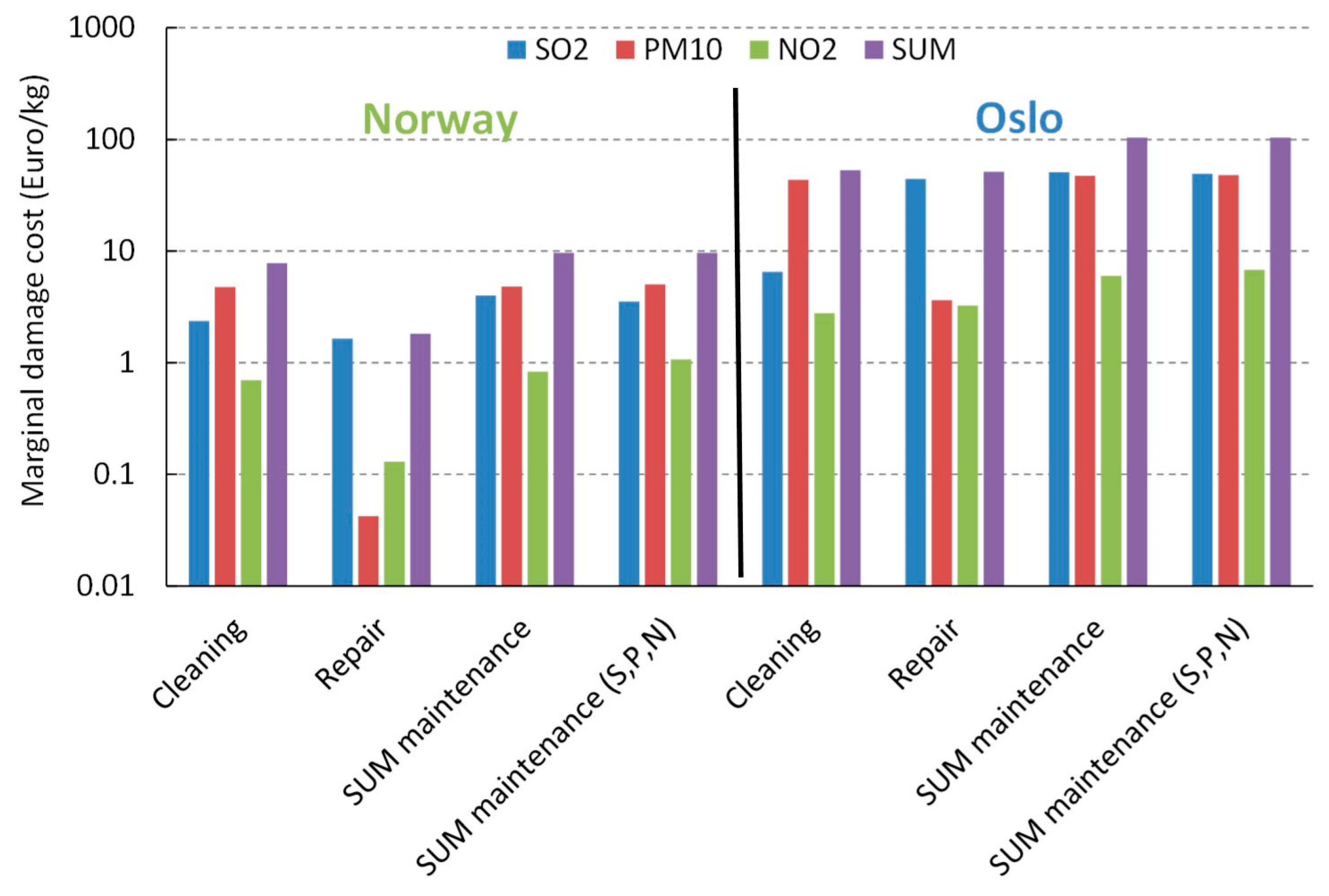
• Direct comparisons of marginal cost estimates for Norway should be for the same selection of the building stock. One reason for present higher costs would be the considerably larger total stock of Norwegian building façades today than in the 1990s. In addition, the values reported in the 1990s were for the ”regional stock of towns and villages with more than 15000 people,” while the present values were obtained as the area averaged, and thus, as the “regional” costs for the total Norwegian building stock. This it not a direct comparison. Clearly, the value for the building density (f_uni, Equation (3)) is important for the results. It may be as relevant to do a regional estimation for Norway for the building stock outside of the cities, as in the earlier report for Norway. The statistics in Norway for areas covered by buildings [33] is by county and municipality and do not distinguish between more or less building-dense areas. However, the statistics [34] show that 82% of the population live in urban settlements, also described as “densly” as opposed to “sparsly” populated areas. If assuming that the distributon of the built surface area reflect the population density, the background façade density, f_uni (Table 2), would be 0.0052 m² façade area/m² land area. This would imply a redution to 18% of the cost values in Table 6. The marginal cost for the façade renovation due to air pollution in Norway, outside of the cities and towns, would then be 1.7 Euro/kg, about equally divided beween the effect of SO₂ (0.72 Euro/kg) and PM₁₀ (0.86 Euro/kg). These values are closer to the range of the earlier reporting (of 0.2–0.5 Euro/kg SO₂), but seem to include less of the buildings than the inventory for “towns and villages with more than 15000 people” used in the 1990s. This may, however, be more or less “compenesated” by the total increased stock. This suggests that a lower building density could have been used in the estimations for Norway. For Oslo the difference is less: the higher repair value, of 51 Euro per kg SO₂ estimated in this work as opposed to 13 Euro per kg SO₂ reported for the 1990s, is, again, probably related to the definition of the building stock. The Oslo municipality area is considerably larger and with a lower average building surface density than the central area with a unity building surface density used in this work. (+, ↑ in Norway)
• The uncertainty in the UWM modelling may be different for the special case of Norway and Europe. The dispersion and deposition of the air pollution relative to the distribution of the building stock in the Norwegian geography could influence the overall impact of the air pollution differently than asssumed in the UWM modelling, and give an undetermined bias in the results estimated in this work. (−)
• Higher values for the marginal costs are expected at the present lower concentration of air pollution in Norway than the French case, as can be seen from the expressions for the impact slopes in Appendix A. The average concentration of PM₁₃ was 32.4 µg/m³ in the French case, and an SO₂ concentration of 19 µg/m³ was reported for the “study of the cost of building renovation due to air pollution in Paris” in the 1990s [1]. In the ICP materials project, an annual average concentration of NO₂ of 70 µg/m³ was measured in Paris in 1997 [35]. For the present Norwegian situation, an increase in the air pollution to these values (for Paris in the 1990s), in an elsewise similar 2020 environment (Table 3), would imply a reduction in the total marginal cost (per unit air pollution) of 44%, of which 90% would be due to a reduction in the marginal cleaning cost for windows (Equation (A4)) and none due to the cleaning of façades due to the applied simple linear Equation (A2). The reduction in the marginal cleaning costs due to PM₁₀, SO₂, and NO₂, would be 25%, 61%, and 84%. One could hypothesize that a further development of the ERF for façade soiling would include a non-linear dependence on the air pollution also in this case. (+)
• The top-down estimates for France in 1994 seem not, in general, to include window cleaning, which constituted 13% of the calculated marginal cleaning cost in Oslo and 45% in Norway (Table 5). (+)
• It may be that the ERFs and maintenance tolerances suggested in the literature and used in this work for the cleaning and repair do not represent the real situation in Norway. The cleaning was supposed to happen as soon as a white painted façade had been soiled to a 35% loss of its original light reflection. Clearly, only few façades are originally white and smooth, and consistently cleaned to remain so. For darker façades, the maintenance tolerance may be higher. (↑)
• Painted façades are a large fraction of the stock at risk (Table 4). It is a question how well the ERFs (Equations (A14), (A17), (A18) and (A20)), which were developed more than 20 years ago in a situation with higher SO₂ concentrations than today and for typical paint systems used at that time, represent the present situation. With the present relatively higher photo-oxidizing impacts of O₃ and NO₂, as compared to the historically higher acidic impact of SO₂, and with expected improved paint systems, it may be that the marginal cost of the air pollution is lower than 20 years ago. This is especially relevant for the ERF for painted steel (Equation (A17)), which includes a reported minimal initial lifetime before cracking (see Section 5.2). (↑)
• The materials inventory is important for the result, as is seen by comparing the cost for the maintenance of the single façade materials for the two Oslo scenarios in Table 5. The definition of the maintenance tolerances, and the renovation works and their pricing, is also important. (−)
• A final consideration is that recorded expenses are not a direct validation of costs. Budgetary constraints may reduce the spending. Whatever the maintenance tolerance is, it may be that the cleaning is in reality less frequent, due to priorities in budgets. For France in 1994 [1] it was reported that about 25% of the recorded renovation expenditure per measured concentration unit of PM₁₃ could be attributed to particle pollution, and was thus included in the reported cost values, of 0.1 Euro per person × year × µg/m³ (1994 value). Income differences explained much of the remaining variation in the cleaning expenses, between 0.1 and 0.4 Euro per person × year × µg/m³. Thus, ~75% of the variation in the cleaning expenses were explained by different factors than the PM concentration. One the one hand, this shows the need in top-down studies to control for other influencing factors on the spending, than air pollution. On the other hand, it is a suggestive indication of the possible difference between bottom-up estimated marginal damage costs due to atmospheric wear, and the expenses it may explain. This is because the air pollution is usually “only” one reason for the wear and the spending, and the price paid for actual renovation include the cost for all other impacts and concerns, which may more or less substitute, and not simply add to, the effect of air pollution. (−)

If the value in Table 6, for Norway is multiplied with 2 to include the amenity loss (see Introduction), this would give about similar marginal renovation costs in Norway due to exposure to SO₂, of 8 (×/÷ 2.5) Euro/kg emission, and due to PM₁₀ of 9.6 (×/÷ 2.5) Euro/kg emission. This marginal cost is much higher than the values reported for the cost in Norway and expenses in France in the 1990s, between 0.1 and 0.55 (1.0, when including the amenity cost) Euro/kg emission. It seems that more than 50% of the difference in the cost due to PM, could be explained by the lower present pollution values (point 3), the inclusion of window cleaning (point 4), and possibly a higher real world maintenance tolerance than applied in the estimations for the cleaning of non-white and non-smooth façades (point 5). There is additional uncertainty in how well the ERFs represent present façades such as the painted steel (point 6), and in the values for other input-parameters to the cost estimations (point 7). The remaining difference is probably related mostly to the amount and selection of the total building stock (point 1) and possibly also to the use of the UWM in Norway (point 2), and to the assessment of other possible influences on the costs and expenses than the atmospheric wear (point 8).

6. Final Remarks and Conclusions

Bottom-up estimates of façade renovation costs due to air pollution can be validated with top-down records of renovation expenses, when the proper control for different influencing factors (than air pollution) and for biases, both on the bottom-up and top-down estimates, is performed.

A disadvantage with the bottom-up method is the very resource- and time-demanding experimental procedure for the development of ERFs. The methodology is very useful in showing trends and comparing between locations, but it is a risk that the environmental situation and the façade materials change more quickly than the experimental method can follow, and that experimentally developed ERFs cannot sufficiently well describe the life time evolution of complex façades. It also depends on uncertain values for the maintenance tolerances and prices, which can be difficult to compare between cases. In addition, the calculation of costs from the weathering effect of air pollution, may not represent the true spending due to the air pollution. This is because other influences on maintenance decisions may not simply add to the effect of air pollution.

A difficulty with the top-down method is to obtain (sufficiently) complete records for the expenses and data for the environmental and other factors which influence the spending.

There are few reported values for marginal cost in the literature and few validation studies have been performed. Due to the many influencing factors, and the need to control for other maintenance reasons than the air pollution, the uncertainty is considerable and difficult to avoid. This is unfortunate for policy application. More studies would be needed both to improve the input values in bottom-up and top-down estimations. Still, due to the many influencing factors and “control-problems,” it seems important to apply similar methods in calculations when comparisons between effects and costs on, for example, health and buildings is needed.

Even if total costs due to air pollution has decreased much over the last decennia, this may not be so for the marginal costs, of which the effect may, however, now be masked by, for example, climate effects. As the marginal costs of air pollution, and thus, the benefit which can be obtained by each unit concentration reduction, can be higher at lower values for the air pollution, it is important to reduce the air pollution as much as possible. However, efforts to reduce low remaining levels of the air pollution may be discouraged by cost-benefit analysis as the mitigation costs of its reduction would generally also be higher at lower levels of the pollution. However, the realization of co-benefits could be important, as for example in the large present effort to electrify the Norwegian road vehicle fleet. The main argument for this is the reduction of CO₂ greenhouse gas emissions, but this is supported by the argument to reduce local PM and NO_x emissions.

The marginal damage costs for cleaning, repair, and in total (cleaning + repair) were found in this work to be, respectively, in Norway: 8, 2, and 10, and in Oslo: 50 (77), 50 (28), and 100 (105) Euro/kg emission, of PM₁₀, SO₂, and NO₂ in total, with an uncertainty range of 2.5 (×/÷ 2.5) these values. For Oslo, the values represent a recorded façade materials inventory for 17–18th century buildings, and in the brackets the same inventory as for Norway. The total marginal costs were shared about equally between the impact of PM₁₀ and SO₂ in Norway (50 and 42% of the impact) and for the 17–18th century buildings in Oslo (45 and 49% of the impact). For a similar façade materials inventory in Oslo as Norway, the total marginal cost due to PM₁₀ was about two-thirds, and that due to SO₂ about one-third of the total, with about 5% of the cost still being due to NO₂.

The division of the costs between cleaning and repair was found to be significantly different in Norway and Oslo. In Norway about 60% of the marginal cleaning cost was found to be due to PM₁₀, 30% due to SO₂, and 10% due to NO₂. In Oslo, about 85% of the cleaning cost was found to be due to PM₁₀, 10% due to SO₂, and 5% due to NO₂. For the marginal repair cost the opposite situation was found, in both Norway and Oslo, with 80–90% of the cost being due to SO₂, 5–10% due to PM₁₀, and 5–10% due to NO₂.

These values are for the total Norwegian building stock, averaged over the country. The selection of the building stock is important. With a definition of a case for Norway, with only the regional building stock included, the costs would be lower. Possible technical biases in the calculations would more probably be towards lower than higher values. As other factors than air pollution deteriorates façades and influences decisions to maintain, the expenses that can be attributed to the air pollution could be significantly lower.

References

1. Rabl, A.; Spadaro, J.V.; Holland, M. How Much is Clean Air Worth? Calculating the Benefits of Pollution Control; Cambridge University Press: Cambridge, UK, 2014. [Google Scholar]
2. ICP. Available online: http://www.corr-institute.se/ICP-Materials/ (accessed on 26 May 2020).
3. Tidblad, J.; Faller, M.; Grøntoft, T.; Kreislova, K.; Varotsos, C.; De la Fuente, D.; Lombardo, T.; Doytchinov, S.; Brüggerhof, S.; Yates, T. Economic Assessment of Corrosion and Soiling of Materials Including Cultural Heritage. UN/ECE International Co-Operative Programme on Effects on Materials, Including Historic and Cultural Monuments. Report no. 65. 2010. Available online: http://www.corr-institute.se/icp-materials/web/page.aspx?refid=18 (accessed on 25 June 2020).
4. EEA. Air Quality in Europe—2018 Report. EEA Report No 12. 2018. Available online: https://www.eea.europa.eu/publications/air-quality-in-europe-2018 (accessed on 26 May 2020).
5. WHO. Review of Evidence on Health Aspects of air Pollution—REVIHAAP Project Technical Report; The WHO European Centre for Environment and Health, WHO Regional Office for Europe: Bonn, Germany, 2013; Available online: http://www.euro.who.int/__data/assets/pdf_file/0004/193108/REVIHAAP-Final-technical-report-final-version.pdf?ua=1 (accessed on 26 May 2020).
6. WHO. Air Quality Guidelines Global Update 2005. Particulate Matter, Ozone, Nitrogen Dioxide and Sulfur Dioxide. 2005. Available online: http://www.euro.who.int/en/health-topics/environment-and-health/air-quality/publications/pre2009/air-quality-guidelines.-global-update-2005.-particulate-matter,-ozone,-nitrogen-dioxide-and-sulfur-dioxide (accessed on 26 May 2020).
7. Maas, R.; Grennfelt, P. (Eds.) Towards Cleaner Air. Scientific Assessment Report 2016; EMEP Steering Body and Working Group on Effects of the Convention on Long-Range Transboundary Air Pollution: Oslo, Norway, 2016; 50p, Available online: https://www.unece.org/index.php?id=42861 (accessed on 26 May 2020).
8. Mills, G.; Pleijel, H.; Malley, C.S.; Sinha, B.; Cooper, O.R.; Schultz, M.G.; Neufeld, H.; Simpson, D.; Sharps, K.; Feng, Z.; et al. Tropospheric Ozone Assessment Report: Present-day tropospheric ozone distribution and trends relevant to vegetation. Elem. Sci. Anthr. 2018, 6, 47. Available online: https://www.elementascience.org/articles/10.1525/elementa.302/ (accessed on 26 May 2020). [CrossRef]
9. Harmens, H.; Mills, G.; Hayes, F.; Sharps, K.; Frontasyeva, M. The Participants of the ICP Vegetation. Air Pollution and Vegetation; ICP Vegetation Annual Report 2015/2016; ICP Vegetation Programme Coordination Centre, Centre for Ecology & Hydrology, Environment Centre Wales: Bangor, Gwynedd, UK, 2016; Available online: http://nora.nerc.ac.uk/id/eprint/515466/ (accessed on 26 May 2020).
10. Watt, J.; Tidblad, J.; Kucera, V.; Hamilton, R. (Eds.) The Effects of Air Pollution on Cultural Heritage; Springer: New York, NY, USA, 2009; pp. 105–127. [Google Scholar]
11. Brimblecombe, P. The Effects of Air Pollution on the Built Environment; Air Pollution Reviews—Volume 2; Imperial College Press: London, UK, 2003; Available online: https://archive.org/details/PeterBrimblecombeTheEffectsOfAirPollutionOnTheBluit (accessed on 26 May 2020).
12. Söderqvist, T.; Barregård, L.; Johansson, N.; Molnár, P.; Nordänger, S.; Staaf, H.; Svensson, M.; Tidblad, J.; Wallström, J. Effektkedjor och Skadekostnader som Underlag för Revidering av ASEK-Värden för Luftföroreningar, Trafikverket, TRV 2016/2932. 2017. Available online: https://www.trafikverket.se/contentassets/773857bcf506430a880a79f76195a080/forskningsresultat/effektkedjor3.pdf (accessed on 26 May 2020). (In Swedish).
13. Söderqvist, T.; Bennet, C.; Kriit, H.K.; Tidblad, J.; Andersson, J.; Jansson, S.-A.; Svensson, M.; Wallström, J.; Andersson, C.; Orru, H.; et al. Underlag för Reviderade ASEK-Värden för Luftföroreningar. Slutrapport från Projektet REVSEK, Trafikverket. 2019. Available online: https://www.trafikverket.se/contentassets/773857bcf506430a880a79f76195a080/forskningsresultat/effektkedjor3.pdf (accessed on 9 June 2020). (In Swedish).
14. SFT. Marginale Miljøkostnader ved Luftforurensning: Skadekostnader og Tiltakskostnader. 2005. Available online: https://www.miljodirektoratet.no/globalassets/publikasjoner/klif2/publikasjoner/luft/2100/ta2100.pdf (accessed on 26 May 2020). (In Norwegian).
15. Sabbioni, C.; Brimblecombe, P.; Cassar, M. The Atlas of Climate Change Impact on European Cultural Heritage: Scientific Analysis and Management Strategies; Anthem Press: London, UK, 2010. [Google Scholar]
16. Grøntoft, T. Conservation-restoration costs for limestone façades due to air pollution in Krakow, Poland, meeting European target values and expected climate change. Sustain. Cities Soc. 2017, 29, 169–177. [Google Scholar] [CrossRef]
17. Kucera, V.; Tidblad, J.; Kreislova, K.; Knotkova, D.; Faller, M.; Reiss, D.; Snethlage, R.; Yates, T.; Henriksen, J.; Schreiner, M. UN/ECE ICP-materials Dose-response Functions for the Multi-pollutant Situation. Water Air Soil Pollut. Focus 2007, 7, 249–258. [Google Scholar] [CrossRef]
18. Henriksen, J.F.; Anda, O.; Ofstad, T. Case Study of «Kristiania Kvadraturen» in Oslo. EU Project ENV4-CT98 0708 Reach Rationlized Economic Appraisal of Cultural Heritage; NILU OR 26/2001; Norwegian Institute for Air Research: Kjeller, Norway, 2001; Available online: https://www.nilu.no/wp-content/uploads/dnn/26-2001-jfh.pdf (accessed on 26 May 2020).
19. Grøntoft, T. Recent Trends in Maintenance Costs for Façades due to Air Pollution in the Oslo Quadrature, Norway. Atmosphere 2019, 10, 529. [Google Scholar] [CrossRef] [Green Version]
20. Tidblad, J.; Kucera, V.; Mikhailov, A.A.; Henriksen, J.; Kreislova, K.; Yates, T.; Stöckle, B.; Schreiner, M. UN ECE ICP Materials. Dose-response functions on dry and wet acid deposition effects after 8 years of exposure. Water Air Soil Pollut. 2001, 130, 1457–1462. [Google Scholar] [CrossRef]
21. Tidblad, J.; Kucera, V.; Mikhailov, A.A. Statistical Analysis of 8 Year Materials Exposure and Acceptable Deterioration and Pollution Levels. UN/ECE International Co-Operative Programme on Effects on Materials, Including Historic and Cultural Monuments. Report no. 30. 1998. Available online: http://www.corr-institute.se/icp-materials/web/page.aspx?refid=18 (accessed on 25 June 2020).
22. Henriksen, J.F.; Anda, O.; Bartonova, A.; Arnesen, K.; Elvedal, U. Evaluation of Decay of Painted Systems for Wood, Steel and Galvanized Steel after 8 Years Exposure. UN/ECE International Co-Operative Programme on Effects on Materials, Including Historic and Cultural Monuments. Report no. 25. 1998. Available online: http://www.corr-institute.se/icp-materials/web/page.aspx?refid=18 (accessed on 25 June 2020).
23. ICP. Oral Communication within ICP-Materials. In Proceedings of the Minutes of the Annual ICP-Materials Meeting, Hämeenlinna, Finland, 10–12 May 2017; Available online: http://www.corr-institute.se (accessed on 26 May 2020).
24. Grøntoft, T.; Verney-Carron, A.; Tidblad, J. Cleaning Costs for European Sheltered White Painted Steel and Modern Glass Surfaces Due to Air Pollution Since the Year 2000. Atmosphere 2019, 10, 167. [Google Scholar] [CrossRef] [Green Version]
25. Statsitics Norway. Index of Labour Costs. 2020. Available online: https://www.ssb.no/en/statbank/table/07251/ (accessed on 26 May 2020).
26. Kucera, V.; EU project Multi Assess. Deliverable 0.2, Publishable Final Report. 2005. Available online: http://www.corr-institute.se/icp-materials/web/page.aspx?refid=35 (accessed on 26 May 2020).
27. Grøntoft, T. Maintenance costs for European zinc and Portland limestone surfaces due to air pollution since the 1980s. Sustain. Cities Soc. 2018, 39, 1–15. [Google Scholar] [CrossRef]
28. Statistics Norway Land Use and Land Cover, 1 January 2016. 2020. Available online: https://www.ssb.no/en/natur-og-miljo/statistikker/arealstat/aar/2016-09-12 (accessed on 26 May 2020).
29. Watt, J.; Jarrett, D.; Hamilton, R. Dose-Response functions for the soiling of heritage materials due to air pollution exposure. Sci. Total Environ. 2008, 400, 415–424. [Google Scholar] [CrossRef] [PubMed]
30. Reichert, T.; Pohsner, U.; Ziegahn, K.-F.; Fitz, S.; Anshelm, F.; Gauger, T.; Schuster, H.; Droste-Franke, B.; Friedrich, R.; Tidblad, J. Effect of Modern Environments on materials—Polymers, Paints and Coatings. In Cultural Heritage in the City of Tomorrow. Developing Policies to Manage the Continuing Risks from Air Pollution. Proceedings of a UNECE Workshop, Bulletin 110E, ISBN 91-87400-12-X, London, UK, 10–12 June 2004; Kucera, V., Tidblad, J., Hamilton, R., Eds.; Swedish Corrosion Institute: Stockholm, Sweden, 2004; ISBN 91-87400-12-X. [Google Scholar]
31. Reichert, T.; Pohsner, U.; Natural Weathering of Polymers. Dose-Response-Functions of Air Pollution Effects for Service Life Prediction. 2006. Available online: http://www.ceees.org/downloads/workshops/pdf/SEE_CEEES_Workshop_2006_Reichert.pdf (accessed on 26 May 2020).
32. OECD. Stat. Organisation for Economic Co-operation and Development. 2020. Available online: https://stats.oecd.org/# (accessed on 26 May 2020).
33. Statistics Norway. Land Use and Land Cover. 2020. Available online: https://www.ssb.no/en/statbank/table/10781/ (accessed on 26 May 2020).
34. Statistics Norway. Population and Land Area in Urban Settlements. 2020. Available online: https://www.ssb.no/en/befolkning/statistikker/beftett (accessed on 26 May 2020).
35. Tidblad, J.; Grøntoft, T.; Kreislová, K.; Faller, M.; De la Fuente, D.; Yates, T.; Verney-Carron, A. Trends in Pollution, Corrosion and Soiling 1987–2012. UN/ECE International Co-Operative Programme on Effects on Materials, Including Historic and Cultural Monuments. Report no. 76. 2014. Available online: http://www.corr-institute.se/icp-materials/web/page.aspx?refid=18 (accessed on 25 June 2020).
36. Lombardo, T.; Ionescu, A.; Chabas, A.; Lefèvre, R.-A.; Ausset, P.; Candau, Y. Dose–response function for the soiling of silica–soda–lime glass due to dry deposition. Sci. Total Environ. 2010, 408, 976–984. Available online: https://www.sciencedirect.com/journal/science-of-the-total-environment/vol/408/issue/4 (accessed on 26 May 2020). [CrossRef] [PubMed]
37. CLRTAP. Mapping of Effects on Materials, Chapter IV of Manual on Methodologies and Criteria for Modelling and Mapping Critical Loads and Levels and Air Pollution Effects, Risks and Trends. UNECE Convention on Long-range Transboundary Air Pollution. 2014. Available online: https://www.umweltbundesamt.de/sites/default/files/medien/4292/dokumente/ch4-mapman-2016-05-03.pdf (accessed on 26 May 2020).
Figure 1. (a) Slopes of the ERFs (SERF,p,i, 1/year × kg/m3), and (b) the marginal cost of the maintenance of the façade materials (SERF,p,i × P, Euro/m2 × year × µg/m3) for the air pollutants SO2 (S), PM10 (P), and NO2 (N), in Norway and Oslo.
Atmosphere 11 00686 g001
Figure 2. The marginal maintenance cost, Dp,i, for the façade materials per kg emission of the air pollutants SO2 (S), PM10 (P), and NO2 (N) (Euro/kg), in Norway and Oslo. The maintenance costs were calculated for the façade and window cleaning and repair operations, given in Table 4.
Atmosphere 11 00686 g002
Figure 3. Marginal damage (maintenance) cost per kg emission of air pollutants for the pollution scenarios in Norway and Oslo, for cleaning, repair and maintenance (cleaning and repair) due to soiling and atmospheric chemical wear by influencing pollutants.
Atmosphere 11 00686 g003