Ozone Trends in the United Kingdom over the Last 30 Years


 ,
, 
Abstract
1. Introduction
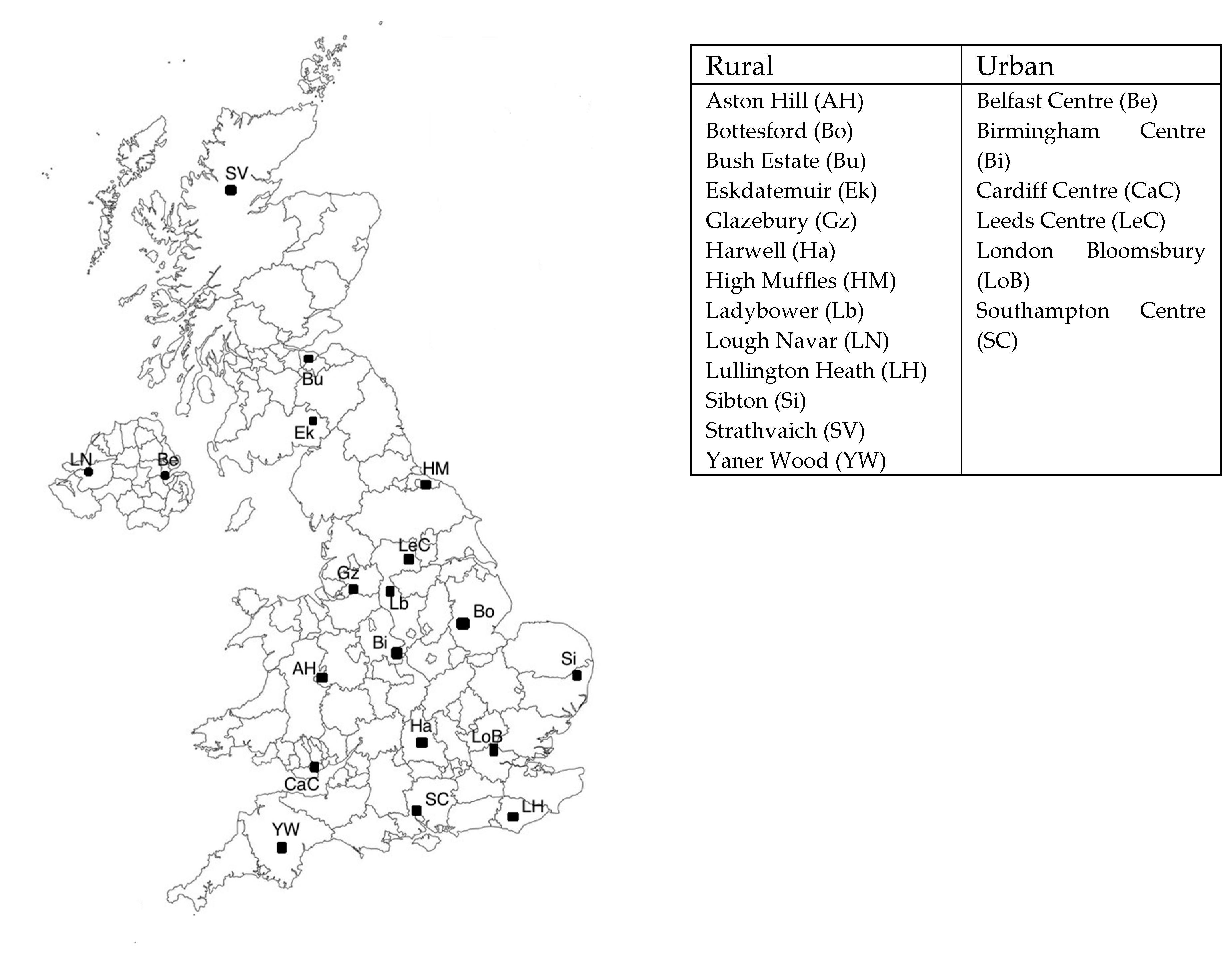
2. Methodology
3. Results and Discussion
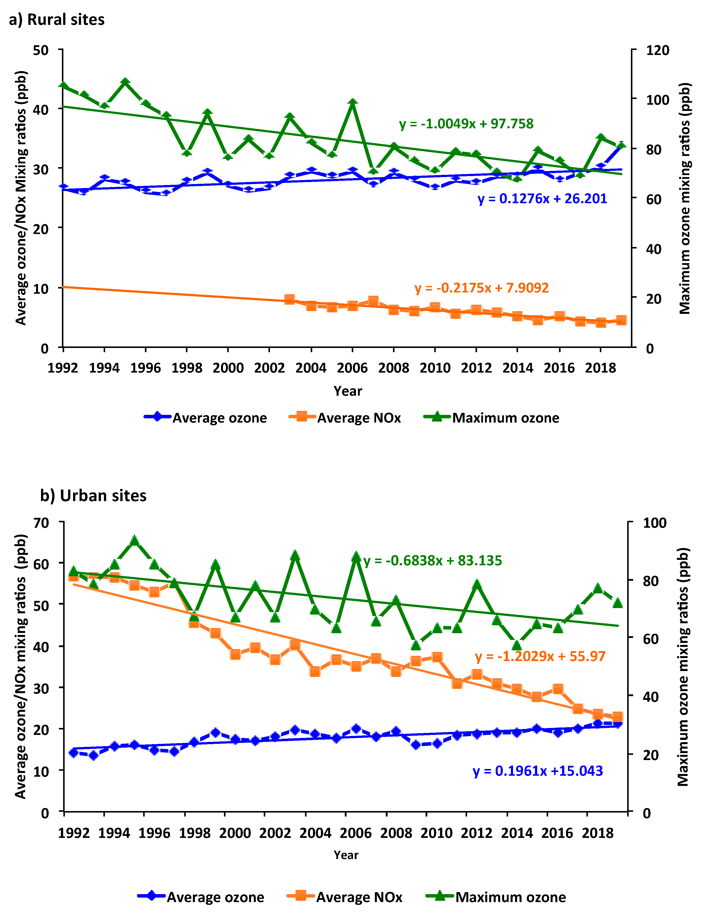
3.1. Three-Decadal Trend of Ozone Mixing Ratios
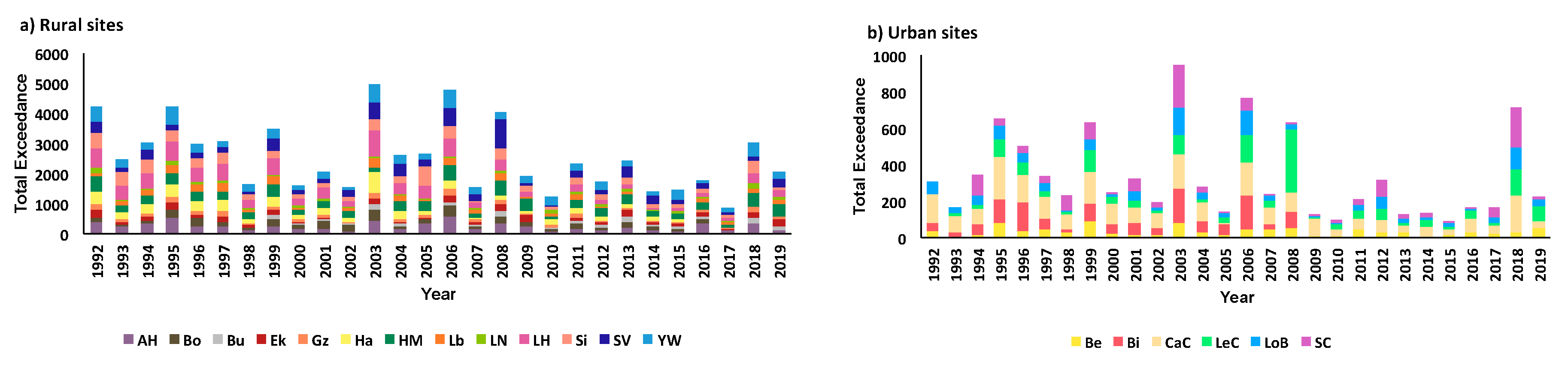
3.2. Yearly Variation of Ozone Exceedances over the Three Decades
3.3. Seasonal Trend Variation of Ozone Exceedances over the Three Decades
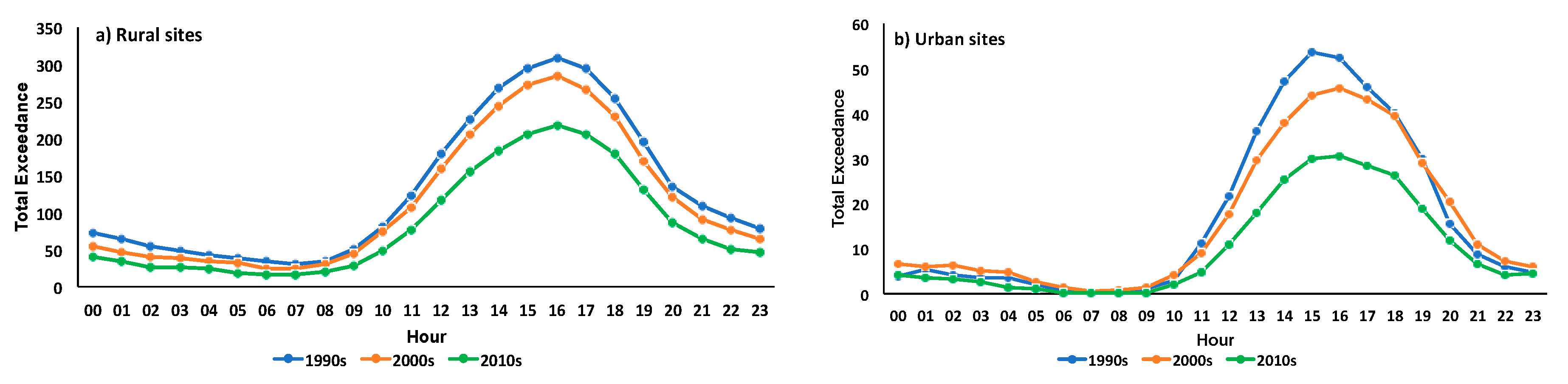
3.4. Daily Variations of Ozone Exceedances over the Three Decades
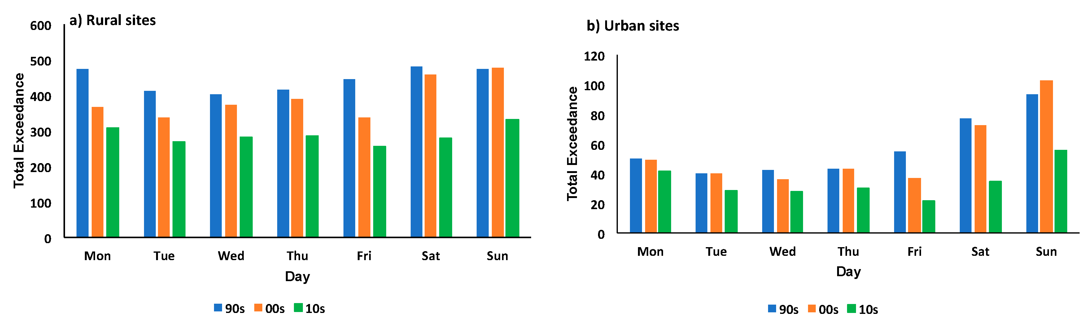
3.5. Weekly Variations of Ozone Exceedances over the Three Decades
3.6. Frequency and Magnitude of Ozone Episodes
Case Study 1
Case Study 2
Case Study 3
4. Conclusions
Supplementary Materials
Author Contributions
Funding
Acknowledgments
Conflicts of Interest
References
- Manahan, S.E. Environmental Chemistry, 8th ed.; CRC Press: Boca Raton, FL, USA, 2005; p. 244. [Google Scholar]
- IPCC (Intergovernmental Panel on Climate Change). Working Group I Contribution to the IPCC Fifth Assessment Report “Climate Change 2013: The Physical Science Basis”, Final Draft Underlying Scientific-Technical Assessment. 2013. Available online: http://www.ipcc.ch (accessed on 18 May 2020).
- Dingenen, R.V.; Dentener, F.J.; Raes, F.; Krol, M.C.; Emberson, L.; Cofala, J. The global impact of ozone on agricultural crop yields under current and future air quality legislation. Atmos. Environ. 2009, 43, 604–618. [Google Scholar] [CrossRef]
- Felzer, B.S.; Cronin, T.; Reilly, J.M.; Melillo, J.M.; Wang, X. Impacts of ozone on trees and crops. Comptes Rendus Geosci. 2007, 339, 784–798. [Google Scholar] [CrossRef]
- Screpanti, A.; De Marco, A. Corrosion on cultural heritage buildings in Italy: A role for ozone? Environ. Pollut. 2009, 157, 1513–1520. [Google Scholar] [CrossRef] [PubMed]
- Zhang, J.; Wei, Y.; Fang, Z. Ozone pollution: A major health hazard worldwide. Front. Immunol. 2019, 10, 2518. [Google Scholar] [CrossRef] [PubMed]
- Heusser, K.; Tank, J.; Holz, O.; May, M.; Brinkmann, J.; Engeli, S.; Diedrich, A.; Framke, T.; Koch, A.; Groβhennig, A.; et al. Ultrafine particles and ozone perturb norepinephrine clearance rather than centrally generated sympathetic activity in humans. Sci. Rep. 2019, 9, 3641. [Google Scholar] [CrossRef]
- Ebi, K.L.; McGregor, G. Climate Change, Tropospheric Ozone and Particulate Matter, and Health Impacts. Environ. Health Perspect. 2008, 116, 1449–1455. [Google Scholar] [CrossRef]
- Lee, S.D.; Wolters, G.J.R.; Grant, L.D.; Schneider, T. Atmospheric Ozone Research and Its Policy Implications; Elsevier: Amsterdam, The Netherlands, 1989; p. 13. [Google Scholar]
- Mazzuca, G.M.; Ren, X.; Loughner, C.P.; Estes, M.; Crawford, J.H.; Pickering, K.E.; Weinheimer, A.J.; Dickerson, R.R. Ozone production and its sensitivity to NOx and VOCs: Results from the DISCOVER-AQ field experiment, Houston 2013. Atmos. Chem. Phys. 2016, 16, 14463–14474. [Google Scholar] [CrossRef]
- Clapp, L.J.; Jenkin, M.E. Analysis of the relationship between ambient levels of O3, NO2 and NO as a function of NOx in the UK. Atmos. Environ. 2001, 35, 6391–6405. [Google Scholar] [CrossRef]
- Paoletti, E.; De Marco, A.; Beddows, D.C.S.; Harrison, R.M.; Manning, W.J. Ozone levels in European and USA cities are increasing more than at rural sites, while peak values are decreasing. Environ. Pollut. 2014, 192, 295–299. [Google Scholar] [CrossRef]
- Monks, P.S.; Archibald, A.T.; Colette, A.; Cooper, O.; Coyle, M.; Derwent, R.; Fowler, D.; Granier, C.; Law, K.S.; Mills, G.E.; et al. Tropospheric ozone and its precursors from the urban to the global scale from air quality to short-lived climate forcer. Atmos. Chem. Phys. 2015, 15, 8889–8973. [Google Scholar] [CrossRef]
- Sicard, P.; Serra, R.; Rossello, P. Spatiotemporal trends in ground-level ozone concentrations and metrics in France over the time period 1999–2012. Environ. Res. 2016, 149, 122–144. [Google Scholar] [CrossRef] [PubMed]
- Khan, M.A.H.; Morris, W.C.; Galloway, M.; Shallcross, B.M.; Percival, C.J.; Shallcross, D.E. An estimation of the levels of stabilized Criegee intermediates in the UK urban and rural atmosphere using the steady-state approximation and the potential effects of these intermediates on tropospheric oxidation cycles. Int. J. Chem. Kinet. 2017, 49, 611–621. [Google Scholar] [CrossRef] [PubMed]
- Jenkin, M. Trends in ozone concentration distributions in the UK since 1990: Local, regional and global influences. Atmos. Environ. 2008, 42, 5434–5445. [Google Scholar] [CrossRef]
- Gaudel, A.; Cooper, O.R.; Ancellet, G.; Barret, B.; Boynard, A.; Burrows, J.P.; Clerbaux, C.; Coheur, P.-F.; Cuesta, J.; Cuevas, E.; et al. Tropospheric Ozone Assessment Report: Present-day distribution and trends of tropospheric ozone relevant to climate and global atmospheric chemistry model evaluation. Elem. Sci. Anth. 2018, 6, 39. [Google Scholar] [CrossRef]
- Directive 2008/50/EC of the European Parliament and of the Council of 21 May 2008 on Ambient Air Quality and Cleaner Air for Europe. Available online: http://data.europa.eu/eli/dir/2008/50/2015-09-18 (accessed on 11 March 2020).
- Air Quality Standards. European Commission—Environment. Available online: https://ec.europa.eu/environment/air/quality/standards.htm (accessed on 11 March 2020).
- Department for Environment Food & Rural Affairs. The Air Quality Strategy for England, Scotland, Wales and Northern Ireland. 2007. Available online: http://www.defra.gov.uk/environment/airquality/strategy/pdf/air-qualitystrategy-vol1.pdf (accessed on 11 March 2020).
- Jenkin, M.; Clemitshaw, K.C. Ozone and other secondary photochemical pollutants: Chemical processes governing their formation in the planetary boundary layer. Atmos. Environ. 2000, 34, 2499–2527. [Google Scholar] [CrossRef]
- Derwent, R.G.; Simmonds, P.G.; Manning, A.J.; Spain, T.G. Trends over a 20-year period from 1987 to 2007 in surface ozone at the atmospheric research station, Mace Head, Ireland. Atmos. Environ. 2007, 41, 9091–9098. [Google Scholar] [CrossRef]
- Jenkin, M.; Davies, T.J.; Stedman, J.R. The origin and day-of-week dependence of photochemical ozone episodes in the UK. Atmos. Environ. 2002, 36, 999–1012. [Google Scholar] [CrossRef]
- Derwent, R.G.; Manning, A.J.; Simmonds, P.G.; Spain, T.G.; O’Doherty, S. Long-term trens in ozone in baseline and European regionally-polluted air at Mace Head, Ireland over a 30-year period. Atmos. Environ. 2018, 179, 279–287. [Google Scholar] [CrossRef]
- National Air Quality Data Archive. Department for Environment Food & Rural Affairs. UK Air Information Resource. Available online: https://uk-air.defra.gov.uk/data/data_selector_service#mid (accessed on 11 March 2020).
- EU Standard Methods for Monitoring and UK Approach, Air Quality Monitoring Methods, Department for Environment Food & Rural Affairs. UK Air Information Resource. Available online: https://uk-air.defra.gov.uk/networks/monitoring-methods?view=eu-standards (accessed on 11 March 2020).
- The Air Quality Data Validation and Ratification Process. Department for Environment Food & Rural Affairs. Available online: https://uk-air.defra.gov.uk/assets/documents/Data_Validation_and_Ratification_Process_Apr_2017.pdf (accessed on 19 December 2019).
- QA/QC Procedures for the UK Automatic Urban and Rural Air Quality Monitoring Network (AURN) Report to Defra and the Developed Administrations (2009) (AEAT/ENV/R/2837). Available online: https://uk-air.defra.gov.uk/assets/documents/reports/cat13/0910081142_AURN_QA_QC_Manual_Sep_09_FINAL.pdf (accessed on 11 March 2020).
- Draxler, R.R.; Rolph, G.D. HYSPLIT (Hybrid Single-Particle Lagrangian Integrated Trajectory) NOAA Air Resourcses Laboratory. Available online: http://www.arl.noaa.gov/ready/hysplit4.html (accessed on 18 May 2020).
- Air Quality Expert Group. Ozone in the United Kingdom. Department for the Environment, Food and Rural Affairs, 2009. Available online: https://uk-air.defra.gov.uk/assets/documents/reports/aqeg/aqeg-ozone-report.pdf (accessed on 18 May 2020).
- Tørseth, K.; Aas, W.; Breivik, K.; Fjaeraa, A.M.; Fiebig, M.; Hjellbrekke, A.G.; Lund Myhre, C.; Solberg, S.; Yttri, K.E. Introduction to the European Monitoring and Evaluation Programme (EMEP) and observed atmospheric composition change during 1972–2009. Atmos. Chem. Phys. 2012, 12, 5447–5481. [Google Scholar] [CrossRef]
- Simpson, D.; Arneth, A.; Mills, G.; Solberg, S.; Uddling, J. Ozone-the persistent menace: Interactions with the N cycle and climate change. Curr. Opin. Environ. Sustain. 2014, 9–10, 9–19. [Google Scholar] [CrossRef]
- Li, Y.; Lau, A.K.H.; Fung, J.C.H.; Zheng, J.; Liu, S. Importance of NOx control for peak ozone reduction in the Pearl River Delta region. J. Geophys. Res. Atmos. 2013, 118, 9428–9443. [Google Scholar] [CrossRef]
- Yan, Y.; Pozzer, A.; Ojha, N.; Lin, J.; Lelieveld, J. Analysis of European ozone trends in the period 1995–2014. Atmos. Chem. Phys. 2018, 18, 5589–5605. [Google Scholar] [CrossRef]
- Solberg, S.; Hov, Ø.; Søvde, A.; Isaksen, I.S.A.; Coddeville, P.; De Backer, H.; Forster, C.; Orsolini, Y.; Uhse, K. European surface ozone in the extreme summer 2003. J. Geophys. Res. Atmos. 2008, 113, D07307. [Google Scholar] [CrossRef]
- Burt, S. The August 2003 heatwave in the United Kingdom Part 1—Maximum temperatures and historical precedents. Weather 2004, 59, 199–208. [Google Scholar] [CrossRef]
- Kendon, M. Has there been a recent increase in UK weather records? Weather 2014, 69, 327–332. [Google Scholar] [CrossRef]
- Nightingale, B.; Allsopp, K. Invasion of Red-footed Falcons in spring 1992. Brit. Birds 1994, 87, 223–231. [Google Scholar]
- Hulme, M. The climate in the UK from November 1994 to October 1995. Weather 1997, 52, 242–257. [Google Scholar] [CrossRef]
- McCarthy, M.; Christidis, N.; Dunstone, N.; Fereday, D.; Kay, G.; Klein-Tank, A.; Lowe, J.; Petch, J.; Scaife, A.; Stott, P. Drivers of the UK summer heatwave of 2018. Weather 2019, 74, 390–396. [Google Scholar] [CrossRef]
- Monks. P.S. A review of the observations and origins of the spring ozone maximum. Atmos. Environ. 2000, 34, 3545–3561. [Google Scholar] [CrossRef]
- Pope, R.J.; Butt, E.W.; Chipperfield, M.P.; Doherty, R.M.; Fenech, S.; Schmidt, A.; Arnold, S.R.; Savage, N.H. The impact of synoptic weather on UK surface ozone and implications for premature mortality. Environ. Res. Lett. 2016, 11, 124004. [Google Scholar] [CrossRef]
- UNECE. The 1999 Gothenburg Protocol to Abate Acidification, Eutrophication and Ground-Level Ozone. Available online: www.unece.org/env/lrtap/multi_h1.htm (accessed on 11 March 2020).
- Hanna, E.; Mayes, J.; Beswick, M.; Prior, J.; Wood, L. An analysis of the extreme rainfall in Yorkshire, June 2007, and its rarity. Weather 2008, 63, 253–260. [Google Scholar] [CrossRef]
- British Isles Weather, June 2011. University of Reading, Department of Meteorology. Available online: http://www.met.rdg.ac.uk/~brugge/diary2011.html#201106 (accessed on 12 March 2020).
- Jaroszweski, D.; Hooper, E.; Baker, C.; Chapman, L.; Quinn, A. The impacts of the 28 June 2012 storms on UK road and rail transport. Meteorol. Appl. 2015, 22, 470–476. [Google Scholar] [CrossRef]
- Parry, S.; Barker, L.; McKenzie, A.; Clemas, S. Hydrological Summary for the United Kingdom June 2013. NERC/Centre for Ecology and Hydrology. Available online: http://nora.nerc.ac.uk/id/eprint/502622/1/HS201306.pdf (accessed on 12 March 2020).
- Parry, S.; Barker, L.; McKenzie, A.; Clemas, S. Hydrological summary for the United Kingdom June 2014. NERC/Centre for Ecology and Hydrology. Available online: http://nora.nerc.ac.uk/id/eprint/507823/1/HS_201406.pdf (accessed on 12 March 2020).
- Kendon, M.; McCarthy, M.; Jevrejeva, S.; Matthews, A.; Legg, T. State of the UK Climate 2015. Met Office: Exeter, UK. Available online: https://www.metoffice.gov.uk/binaries/content/assets/metofficegovuk/pdf/weather/learn-about/uk-past-events/state-of-uk-climate/mo-state-of-uk-climate-2015-v3.pdf (accessed on 12 March 2020).
- Kendon, M.; McCarthy, M.; Jevrejeva, S.; Matthews, A.; Legg, T. State of the UK Climate 2016. Met Office: Exeter, UK. Available online: https://www.metoffice.gov.uk/binaries/content/assets/metofficegovuk/pdf/weather/learn-about/uk-past-events/state-of-uk-climate/mo-state-of-uk-climate-2016-v4.pdf (accessed on 12 March 2020).
- Kendon, M.; McCarthy, M.; Jevrejeva, S.; Matthews, A.; Legg, T. State of the UK climate 2017. Int. J. Clim. 2018, 38, 1–35. [Google Scholar] [CrossRef]
- Kendon, M.; McCarthy, M.; Jevrejeva, S.; Matthews, A.; Legg, T. State of the UK climate 2018. Int. J. Clim. 2019, 39, 1–55. [Google Scholar] [CrossRef]
- Wet Weather June 2019. Met Office. Available online: https://www.metoffice.gov.uk/binaries/content/assets/metofficegovuk/pdf/weather/learn-about/uk-past-events/interesting/2019/2019_006_rainfall_lincolnshire.pdf (accessed on 19 December 2019).
- Shukla, J.B.; Misra, A.K.; Sundar, S.; Naresh, R. Effect of rain on removal of a gaseous pollutant and two different particulate matters from the atmosphere of a city. Math. Comp. Model. 2008, 48, 832–844. [Google Scholar] [CrossRef]
- Garland, J.A. and Derwent, R.G. Destruction at the ground and the diurnal cycle of concentrations of ozone and other gases. Q. J. R. Meteorol. Soc. 1979, 105, 169–183. [Google Scholar] [CrossRef]
- Sillman, S. The relation between ozone, NOx and hydrocarbons in urban and polluted rural environments. Atmos. Environ. 1999, 33, 1821–1845. [Google Scholar] [CrossRef]
- Galbally, I.E.; Roy, C.R. Destruction of ozone at the Earth’s surface. Q. J. R. Meterol. Soc. 1980, 106, 599–620. [Google Scholar] [CrossRef]
- Henry, R.F. Weekday/weekend differences in gasoline related hydrocarbons at coastal PAMS sites due to recreational boating. Atmos. Environ. 2013, 75, 58–65. [Google Scholar] [CrossRef]
- Kent, A. Air Pollution Forecasting: Ozone Pollution Episode Report (August 2003). Department for Environment Food & Rural Affairs, UK. Available online: https://uk-air.defra.gov.uk/assets/documents/reports/cat12/o3_episode_august2003.pdf (accessed on 18 May 2020).
- Prior, J.; Beswick, M. The record breaking heat and sunshine of July 2006. Weather 2007, 62, 174–182. [Google Scholar] [CrossRef]
- UK Weather: Hottest Easter Monday on Record. BBC News. 22 April 2019. Available online: https://www.bbc.co.uk/news/uk-48013791 (accessed on 12 March 2020).
- Storm Hannah 26 to 27 April 2019. Met Office. Available online: https://www.metoffice.gov.uk/binaries/content/assets/metofficegovuk/pdf/weather/learn-about/uk-past-events/interesting/2019/2019_005_storm_hannah.pdf (accessed on 12 March 2020).


| Type of Site | 1990s | 2000s | 2010s | Overall |
|---|---|---|---|---|
| Rural | 1941 | 2141 | 1412 | 5494 |
| Urban | 532 | 647 | 376 | 1554 |
| Year | Month | Duration (days) | Highest Mixing Ratios (ppb) | Site Type | Location |
|---|---|---|---|---|---|
| 1992 | May and June | 16 and 9 + 9 a | 125 and 125 | Rural | Ha and Si |
| 1995 | August | 17 | 133 | Rural | YW |
| 1995 | May and August | 6 and 3 + 4 d | 104 and 102 | Urban | LoB and CaC |
| 1999 | July | 4 | 94 | Urban | CaC |
| 2003 | August | 8 | 108 | Rural | Ha and LH |
| 2003 | August | 7 | 116 | Urban | SC |
| 2006 | July | 4 + 7 b | 114 | Rural | LH |
| 2006 | July | 4 | 101 | Urban | CaC |
| 2008 | May | 26 or 8 + 9 c | 89 | Rural | AH and YW |
| 2008 | May | 27 or 9 + 10 e | 90 | Urban | CaC |
| 2018 | May | 11 | 89 | Rural | YW |
| 2018 | May | 8 | 89 | Urban | SC |
| 2019 | April | 13 | 87 | Rural | HM |
| 2019 | April | 5 | 79 | Urban | LeC |
| Sites | Case Study 1 August 2003 | Case Study 2 July 2006 | Case Study 3 April 2019 | |||
|---|---|---|---|---|---|---|
| Days | O3 (ppbv) | Days | O3 (ppbv) | Days | O3 (ppbv) | |
| AH | 9 | 79.5 | 6 | 112 | 10 | 77.4 |
| Bo | 11 | 99.9 | 11 | 95.8 | N/A | N/A |
| Bu | 5 | 66.3 | 3 | <50 | 6 | 74.1 |
| Ek | 5 | 74.4 | 5 + 5 | 89.7 | 16 | 78.2 |
| Gz | 6 | 88.7 | 5 + 7 | 95.8 | 6 | 73.5 |
| Ha | 14 | 108.0 | 5 + 8 | 105.0 | N/A | N/A |
| HM | 7 | 68.3 | 6 + 7 | 71.3 | 16 | 86.3 |
| Lb | 11 | 88.7 | 5 + 6 | 70.3 | 7 | 81.5 |
| LN | 5 | 55.0 | 2 | 86.6 | 16 | 78.2 |
| LH | 10 | 108.0 | 5 + 8 | 114.2 | 14 | 76.0 |
| Si | 11 | 79.5 | 6 + 14 | 89.7 | 5 | 77.9 |
| SV | 4 | 75.4 | 2 + 3 | 92.8 | 8 | 75.7 |
| YW | 10 | 89.7 | 2 + 7 | 99.9 | 8 | 70.4 |
| Be | 4 | 65.2 | 3 | 95.8 | 5 | 76.5 |
| Bi | 1 | 68.3 | 6 | 85.6 | N/A | N/A |
| CaC | 9 | 85.6 | 5 | 100.9 | 4 | 72.9 |
| LeC | 8 | 70.3 | 4 | 78.5 | 8 | 78.9 |
| LoB | 6 | 90.7 | 5 | 90.7 | 4 | 61.9 |
| SC | 10 | 116.2 | 3 | 76.4 | 3 | 54.6 |
© 2020 by the authors. Licensee MDPI, Basel, Switzerland. This article is an open access article distributed under the terms and conditions of the Creative Commons Attribution (CC BY) license (http://creativecommons.org/licenses/by/4.0/).
Share and Cite
Diaz, F.M.R.; Khan, M.A.H.; Shallcross, B.M.A.; Shallcross, E.D.G.; Vogt, U.; Shallcross, D.E. Ozone Trends in the United Kingdom over the Last 30 Years. Atmosphere 2020, 11, 534. https://doi.org/10.3390/atmos11050534
Diaz FMR, Khan MAH, Shallcross BMA, Shallcross EDG, Vogt U, Shallcross DE. Ozone Trends in the United Kingdom over the Last 30 Years. Atmosphere. 2020; 11(5):534. https://doi.org/10.3390/atmos11050534
Chicago/Turabian StyleDiaz, Florencia M. R., M. Anwar H. Khan, Beth M. A. Shallcross, Esther D. G. Shallcross, Ulrich Vogt, and Dudley E. Shallcross. 2020. "Ozone Trends in the United Kingdom over the Last 30 Years" Atmosphere 11, no. 5: 534. https://doi.org/10.3390/atmos11050534
APA StyleDiaz, F. M. R., Khan, M. A. H., Shallcross, B. M. A., Shallcross, E. D. G., Vogt, U., & Shallcross, D. E. (2020). Ozone Trends in the United Kingdom over the Last 30 Years. Atmosphere, 11(5), 534. https://doi.org/10.3390/atmos11050534