Article

Time Series Analysis and Forecasting Using a Novel Hybrid LSTM Data-Driven Model Based on Empirical Wavelet Transform Applied to Total Column of Ozone at Buenos Aires, Argentina (1966–2017)

by
Nkanyiso Mbatha
1,* and
Hassan Bencherif
2,3
1
Department of Geography, University of Zululand, KwaDlangezwa 3886, South Africa
2
Laboratoire de l’Atmosphère et des Cyclones, LACy UMR 8105, Université de la Réunion, 97400 Réunion Island, France
3
School of Chemistry and Physics, University of KwaZulu-Natal, Private Bag X54001, Durban 4000, South Africa
*
Author to whom correspondence should be addressed.
Atmosphere 2020, 11(5), 457; https://doi.org/10.3390/atmos11050457
Submission received: 7 April 2020 / Revised: 25 April 2020 / Accepted: 25 April 2020 / Published: 30 April 2020
(This article belongs to the Special Issue Ozone Evolution in the Past and Future)

Abstract

:
Total column of ozone (TCO) time series analysis and accurate forecasting is of great significance in monitoring the status of the Chapman Mechanism in the stratosphere, which prevents harmful UV radiation from reaching the Earth’s surface. In this study, we performed a detailed time series analysis of the TCO data measured in Buenos Aires, Argentina. Moreover, hybrid data-driven forecasting models, based on long short-term memory networks (LSTM) recurrent neural networks (RNNs), are developed. We extracted the updated trend of the TCO time series by utilizing the singular spectrum analysis (SSA), empirical wavelet transform (EWT), empirical mode decomposition (EMD), and Mann-Kendall. In general, the TCO has been stable since the mid-1990s. The trend analysis shows that there is a recovery of ozone during the period from 2010 to 2017, apart from the decline of ozone observed during 2015, which is presumably associated with the Calbuco volcanic event. The EWT trend method seems to have effective power for trend identification, compared with others. In this study, we developed a robust data-driven hybrid time series-forecasting model (named EWT-LSTM) for the TCO time series forecasting. Our model has the advantage of utilizing the EWT technique in the decomposition stage of the LSTM process. We compared our model with (1) an LSTM model that uses EMD, namely EMD-LSTM; (2) an LSTM model that uses wavelet denoising (WD) (WD-LSTM); (3) a wavelet denoising EWT-LSTM (WD-EWT-LSTM); and (4) a wavelet denoising noise-reducing sequence called EMD-LSTM (WD-EMD-LSTM). The model that uses the EWT decomposition process (EWT-LSTM) outperformed the other five models developed here in terms of various forecasting performance evaluation criteria, such as the root mean square error (RMSE), mean absolute error (MAE), mean absolute percentage error (MAPE), and correlation coefficient (R).

1. Introduction

Total column of ozone (TCO), defined as the vertical integration of ozone number density profile in the lower and middle atmosphere, is important for regulating the amount of harmful ultraviolet (UV) radiation reaching the surface of the Earth. The decline of global stratospheric ozone column observed throughout the 1980s [1] and the discovery of the Southern Hemisphere polar region ozone hole [2,3] raised the awareness of the need to protect the global ozone layer. The ozone decline and Antarctic ozone hole, which is stronger during the Southern Hemisphere spring, is known to be the result of chemical reactions involving chlorine and bromine, which causes ozone in the southern polar region to be severely depleted. However, the Montreal Protocol, a global agreement initiated in 1987, became a binding agreement designed to protect the ozone layer by phasing out the production of ozone-depleting gases such as chlorofluorocarbons (CFCs).
A number of atmospheric chemistry research groups have been closely monitoring the slow self-recovery of stratospheric ozone for some time. The difficulty of this slow recovery is that the entire process depends solely on the self-recovery aspects of the ozone layer. Consequently, the recovery of the stratospheric ozone layer is strongly dependent on the continued decline in the atmospheric concentration of ozone-depleting gases such as CFC [4]. However, it is concerning that a recent study by Rigby et al. [4] reported that the recent slowing down of the stratospheric ozone layer recovery is counterbalanced by the continual emission of trichlorofluoromethane (CFC-11) in northeast China. The suggestion of a decrease in stratospheric ozone recovery and the continuation of the ozone decline in the lower stratosphere has been presented by other authors [5]. The study by Ball et al. [5] indicated that, while the stratospheric ozone layer has stopped declining across the globe, there is no clear increase observed at latitudes between 60° S and 60° N outside the polar region (60°–90°). Therefore, it is for this reason that TCO time series studies and the consequent design of models that can predict and forecast the dynamics of the ozone concentration in the atmosphere are imperative.
Studies of the time series analysis of satellite and ground-based TCO data revealed a significant decline of −3% to −6% per decade (depending on latitude) throughout the 1980s and 1990s. These were linked to CFCs increases in the atmosphere [6,7]. Chehade at al. [8] investigated the long-term evolution of zonal mean annual mean total ozone measurements (between 65° S and 65° N) from merged data sets of various satellites over a period of 1979–2012. Among other things, their study showed (1) a strong effect of the El Chichón (1982) and Mt. Pinatubo (1991) volcanic eruptions in the global TCO distribution and (2) evidence for a large fraction of ozone loss, which was more prominent in the Northern Hemisphere. Recently, Ball et al. [9] assessed the trend in stratospheric ozone using space-based global ozone observations from 1985 to 2018. Their study demonstrated that large inter-annual mid-latitude variations observed during 2017 resurgence are driven by non-linear quasi-biennial oscillation (QBO) phase-dependent seasonal variability. A year later, Ball et al. [5] quantified the absolute changes in ozone within different regions of the stratosphere and troposphere and speculated, by using a robust regression analysis approach and dynamical linear modeling, on the latitudinal contributions to the total column ozone since 1998. Utilizing multiple satellite data sets in their study, they managed to show evidence that ozone in the lower stratosphere between 60° S and 60° N has continued to decline since 1998.
Data-driven time series forecasting is an important research topic in the domain of science and engineering. The primary objective of this data science domain is to use available data to develop a mathematical model that can forecast future situations. Over the years, there have been many efforts in the development and improvement of time series forecasting models. These models can be classified into statistical models, artificial intelligence models, physical models, and hybrid models [10]. Statistical models like autoregressive integrated moving average (ARIMA) linear models [11] and artificial intelligence models like artificial neural networks (ANN) non-linear models [11,12] are widely popular data-driven time series models. However, a hybrid model [13], which is built by combining the two methods (non-linear and linear), has been shown to produce better results than the individual models [11,14,15,16]. To improve the performance of the hybrid models, signal decomposition is an important step when contracting the model [17,18,19,20]. The most popular methods for signal decomposition include discrete wavelet transform (DWT) [16,19], empirical mode decomposition (EMD), and ensemble empirical mode decomposition (EEMD) [11,21], among others. Recently, a new novel signal decomposition technique was developed, named the empirical wavelet transform (EWT) [22]. This technique integrates systems with a mathematical theory like wavelet transform (WT) and adaptiveness to the signal like EMD. Subsequently, this technique has proven to be efficient in the improvement of the performance of hybrid time series forecasting models [17,18,20].
Long short-term memory networks (LSTM) recurrent neural networks (RNNs), which were proposed by Hochreiter and Schmidhuber [23], have been proven as an enhanced variant of RNNs that can learn the information contained in time series data more robustly. LSTM, a deep learning method, can more effectively capture the variability of time series data compared with other models such as ARIMA and ANN. However, the model accuracy is not high, using the LSTM network in its simplest form, to predict the time series data. Therefore, applying it in its simplest form, in a non-stationary time series data like the TCO time series used here, consideration should be given to first decomposing the time series to several more predictable components, each having less non-stationarity in order to improve overall accuracy. LSTM has been previously used in digital currency forecasting [18], daily land surface temperature forecasting [11], wind speed forecasting [20], and wind power short-term prediction [19], among others.
In this paper, the analysis of the growth rate and trend of the long-term data series of the TCO measured at Buenos Aires for the period from 1966 to 2017 is carried out. This data is one of the longest recorded time series of TCO in the Southern Hemisphere. A number of studies have indicated that the EMD technique can be an important method for trend identification [10,11,12]. This research proposes the use of the EWT technique for the first time to identify the trend of the TCO time series. In addition, the authors aim to develop a robust data-driven hybrid model that uses the EWT technique in the decomposition stage of the LSTM, namely EWT-LSTM, and use this model in forecasting the TCO time series. The EWT-LSTM is subsequently compared to an LSTM model that uses EMD, namely EMD-LSTM. The study also develops the LSTM model that uses wavelet denoised (WD) data (WD-LSTM), wavelet denoising noise reduction EWT-LSTM (WD-EWT-LSTM), and wavelet denoising EMD-LSTM (WD-EMD-LSTM). Finally, statistical evaluation metrics (i.e., root mean square error (RMSE), mean absolute error (MAE), mean absolute percentage error (MAPE), and R) were used to assess the performance of the above-mentioned models, including a single LSTM model.

2. Materials and Methods

2.1. Total Column Ozone

The total column of ozone (TCO) data used in this paper are the long record of Dobson observations, measured at Observatorio Central Buenos Aires (OCBA) (34.60° S, 58.38° W) for the period from 1966 to 2017 [24], which was downloaded from the World Ozone and Ultraviolet Radiation Data Centre website (https://woudc.org/home.php). The Dobson spectrometer instrument was developed by G. M. B. Dobson [25]. Since then, this instrument played an instrumental role in the measurements of TCO in different locations around the Earth. It is also important to mention here that the first observation of the Antarctic ozone hole was observed by a Dobson instrument [2], and later confirmed by total ozone mapping spectrometer (TOMS) instrument [26]. The Dobson measurement method is based on the use of ozone absorption in the Huggins band. Owing to the possible interference by aerosols and molecules, the differential absorption at two wavelength pairs is measured to separate the ozone absorption from aerosols and molecules in the atmosphere. More details about Dobson spectrometers and its accuracy assessment can be found in a study by Grant [27].

2.2. Mann-Kendal

It is always vital to work out monotonic trends in the time series of any geophysical data before any advance use. In this study, the Mann-Kendall test [28,29] was used to detect the trends that exist among the used variables. This method is defined as a non-parametric, rank-based method that is commonly used to extract monotonic trends in the time series of climate data, environmental data, or hydrological data. The following formula (Equation (1)) is used to compute Mann-Kendall test statistics:
S = k = 1 n 1   j = k + 1 n s g n ( X j X k )
where
s g n ( x ) = { + 1 , if   x > 1 0 , if   x = 0 1 , if   x < 1
The average value of S is E [ S ] = 0 , and the variance σ 2 is calculated using the following equation (Equation (3)):
σ 2 = { n ( n 1 ) ( 2 n + 5 ) j = 1 p t j ( t j 1 ) ( 2 t j + 5 ) } / 18
where t j is the number of data points in the j t h tied group, and p is the number of the tied group in the time series. Under the assumption of a random and independent time series, the statistical function S is approximately normal distributed given that the below Z-transformation equation (Equation (4)) is used:
Z = { S 1 σ if   S > 1 0 if   S = 0 S + 1 σ if   S < 1
The value of the statistic S is associated with Kendall’s τ = S D , where
D = [ 1 2 n ( n 1 ) 1 2 j = 1 p t j ( t j 1 ) ] 1 / 2 [ 1 2 n ( n 1 ) ] 1 / 2
In respect to the above-defined Z-transformation equation, this study reflects a 95% confidence level, where the null hypothesis of no trend is rejected if | Z | > 1.96. Another important output of the Mann-Kendall statistic is the Kendall tau “ τ ”, which is a measure of a correlation, which measures the strength of the relationship between any two independent variables. In this study, the Mann-Kendall test system summarized above was applied to the TCO time series under scrutiny.
The limitations of the Mann-Kendall test are that it does not give the complete structure of the trend for the whole time series. Understanding the dynamics of the trend throughout the time series is important as there might be fluctuations in the trend over the investigation period. This limitation is solved by applying the test sequentially for every individual period. This specific version of the Mann-Kendall test statistic is called sequential Mann-Kendall (SQ-MK) [30]. The SQ-MK test method generates two time series, a forward/progressive one (u(t)) and a backward/retrograde one (u’(t)), and is furthermore capable of detecting approximate potential trend turning points in long-term time series, which can be obtained by plotting the progressive and retrograde time series in the same figure. If they happen to cross each other and diverge beyond the specific threshold (±1.96 in this study), then there is a statistically significant trend. To compute SQ-MK, rank values are used. The ranked values of y i of a given time series ( x 1 ,   x 2 , x 3 , , x n ) in the analysis, as well as the magnitudes of y i ,   ( i = 1 , 2 , 3 , , n), are compared with y i ,   ( j = 1 , 2 , 3 , , j − 1). At each comparison, the number of cases where y i > y j is counted and then donated to n i . The statistic t i is thus calculated by the following:
t i = j = 1 i n i
The mean and variance of the statistic t i are given by the following:
E ( t i ) = i ( i 1 ) 4
and
Var ( t i ) = i ( i 1 ) ( 2 i 5 ) 72
The forward/progressive sequential values of the statistic u ( t i ) that are standardized are calculated using the following Equation (30):
u ( t i ) = t i E ( t i ) Var ( t i )
In order to calculate the backward/retrograde statistic values u ( t i ) , the same time series ( x 1 ,   x 2 , x 3 , , x n ) is used, but statistic values are computed by starting from the end of the time series. The plotting of the forward and backward sequential statistic in the same figure allows for the detection of the approximate beginning of a developing trend. It is noteworthy to also mention that, in the SQ-MK trend analysis, sometimes the forward and backward trends cancel each other and finally do not give a significant trend. This method has been successfully employed by many researchers to detect trend turning points and its significance [28,30]. The Mann-Kendall trend test and the SQ-MK trend analysis were performed using package ‘trend’ [31] and ‘pheno’ [32], respectively, run in R version 3.5.0.

2.3. Empirical Mode Decomposition (EMD)

The empirical mode decomposition is a fundamental part of the Hilbert–Huang transform (HHT). The signal is decomposed into so-called intrinsic mode functions (IMFs) that include both the trend and finite oscillations that supply information on different scales of the original signal. This method is a self-adaptive time–space analysis method, designed for processing time series that are non-stationary and non-linear. In mathematical operation, the EMD decomposes the time series as a finite sum of N + 1 IMFs f k ( t ) , such that,
f ( t ) = k = 0 N f k ( t ) .
An IMF is an amplitude modulated-frequency modulated function, which can be mathematically represented in the following form:
f k ( t ) = F k ( t ) cos ( φ k ( t ) )   where   F k ( t ) ,   φ k ( t ) > 0     t .
Following a study by Gilles [22] where they explored the EMD set of equations, in the above equation, it is assumed that f k and φ k vary much slower than φ k . It should also be noted that the IMF parameter f k behaves as a harmonic component. These IMFs are extracted by first computing the upper, f ¯ ( t ) , and the lower, f _ ( t ) , envelopes using a cubic spline interpolation method from the maxima and minima of f . Thereafter, the mean envelop is calculated using the following formula:
m ( t ) = ( f ¯ ( t ) + f _ ( t ) ) 2 ,
and, finally, the IMF candidate is computed as follows:
r 1 ( t ) = f ( t ) m ( t ) .
In normal circumstances, r 1 ( t ) does not fulfill the properties of an intrinsic mode function; hence, an acceptable IMF candidate is reached by iterating the same process to r 1 and the subsequent r k . The ultimate retained IMF is given by the following:
f 1 ( f ) = r n ( f ) ,
Moreover, the next IMF is obtained by the same algorithm applied on f ( t ) f 1 ( t ) . The remaining IMFs are also extracted by repeating this algorithm on the successive residuals. While this algorithm seems to be highly adaptable and able to compute the non-stationary part of the original function, its main problem is that it is based on an ad-hoc process that is mathematically difficult to model [22]. This method also presents limitations when some noise is added in the signal. To solve some of these limitations, an ensemble EMD (EEMD) was proposed in a study by Torres et al. [33]. The key idea of the EEMD relies on averaging the modes obtained by EMD applied to several realizations of Gaussian white noise added to the original signal. The resulting decomposition solves the EMD mode-mixing problem; however, it introduces new ones. In the method proposed here, a particular noise is added at each stage of the decomposition and a unique residue is computed to obtain each mode. The resulting decomposition is complete, with a numerically negligible error. During a study by Gilles [22], this method was tested using two examples, namely a discrete Dirac delta function and an electrocardiogram signal. The results showed the following: (1) compared with EEMD, the new method (EWT) provides a better spectral separation of the modes; and (2) it requires a smaller number of sifting iterations, which reduces the computational cost. It should be noted that a study by Torres et al. [33] showed that the EEMD method does seem to stabilize the obtained EMD decomposition, but with an increase in computational cost. This is one of the reasons this study explored the used of the more theoretical driven EWT method, which is explained in a study by Gilles [22].

2.4. Empirical Wavelet Tranform

Our study proposes the use of a newely developed method (EWT) that is used to decompose any signal into a collection of amplitude modulated-frequency modulated (AM–FM) signals according to the information contained within the Fourier spectrum of the given signal. The method was developed by Gilles [22], and it enables the extraction of different modes of the signal by designing a suitable filter bank. This method is called the empirical wavelet transform. While the EMD is a traditional method that is normally used to decompose a signal according to its contained information within a signal, the main concern about this method is that it lacks mathematical theory. However, the EWT with its well-defined mathematical theory has been shown to perform better than the EMD (e.g., Gilles [22]). When applying the EWT in a time series x ( t ) , the process of signal decomposition can be described in the following five steps:
The first step is to calculate the Fourier spectrum F ( ω ) of the given signal using the fast Fourier transform algorithm.
The second step includes determining the boundaries ω i by proper segmentation of the Fourier spectrum:
ω i = f i + f i + 1 2 for   1 i 1
where { f i } ,   i = 1 , 2 , , N represents the frequencies corresponding to local maxima and f 0 = 0 . The third step is to construct the empirical wavelet ψ i ( ω ) and the empirical scaling function φ i ( w ) in the following form:
φ i ( ω ) = { 1 ,   if   ( 1 + γ ) ω i | ω | ( 1 γ ) ω i + 1 cos [ π 2 β ( 1 2 γ ω i + 1 ( | ω | ( 1 γ ) ω i + 1 ) ) ] ,   if   ( 1 γ ) ω i + 1 | ω | ( 1 + γ ) ω i + 1 sin [ π 2 β ( 1 2 γ ω i ( | ω | ( 1 γ ) ω i ) ) ] ,   if   ( 1 γ ) ω i | ω | ( 1 + γ ) ω i 0 ,     Otherwise
and
φ i ( ω ) = { 1 ,   if   | ω | ( 1 γ ) ω i   cos [ π 2 β ( 1 2 γ ω i ( | ω | ( 1 γ ) ω i ) ) ] ,   if   ( 1 γ ) ω i | ω | ( 1 + γ ) ω i 0 ,     Otherwise
where γ = m i n i ( ω i + 1 ω i ω i + 1 + ω i ) . In both the above equations, the function β ( x ) represents an arbitrary C k ( [ 0 , 1 ] ) function, such that,
β ( x ) = { 1   i f   x 1 0   i f   x 0   and   β ( x ) + β ( 1 x ) = 1     x [ 0 , 1 ]
Most of the functions do satisfy these properties, and studies such as Gilles [22] and Daubechies [34] have shown that the frequently used is as follows:
β ( x ) = x 4 ( 35 84 x + 70 x 2 20 x 4 )
It should be noted that the above equations were reduced to this form after first assuming that the Fourier support [ 0 , π ] is segmented into N contiguous segments (e.g., Gilles [22]). The frequency ω i is then denoted to be the limits between each segment. A detailed procedure followed to produce both the empirical wavelet and empirical scaling function is given in a study by Gilles [22].
The fourth step is to calculate the approximate and detail coefficients using the following equations:
W x ( i , t ) = x ( t ) , ψ i ( t ) = x ( τ ) ψ i ( τ t ) d = F 1 [ x ( ω ) ψ ( ω ) ]
W x ( 1 , t ) = x ( t ) , ψ 1 ( t ) = x ( τ ) ψ 1 ( τ t ) d = F 1 [ x ( ω ) ψ i ( ω )
The final step is to reconstruct the original signal in order to obtain different modes in the following form:
x ( t ) = W x ( 1 , t ) × φ 1 ( t ) + i = 2 N W x ( i , t ) × ψ i ( t )
The details about the EWT contraction process as well as the testing of the method using different signals, including artificial signals and real electrocardiogram signals, is decsribed in Gilles [22]. Recently, Zhou et al. [17] used the EWT technique in a data pre-analysis step in their study of data pre-analysis and ensemble of various artificial neural networks for monthly streamflow forecasting.

2.5. Long Short-Term Memory (LSTM)

The LSTM is a special type of recurrent neural network (RNN) that was proposed by Hochreiter and Shmidhuber [23]. These RNNs are improved multilayer perception networks that are often termed as deep learning, and are somewhat different from traditional artificial neural networks (ANN) [35]. The general architecture of the traditional ANNs employs a feedforward neural network system, which means artificial neural networks with connections between the units do not form a cycle. In other words, in a feedforward network, the processing of information is piped through the network from the input layers to output layers. On the other hand, the RNN is an artificial neural network where connections form between units form cyclic paths. RNNs are defined as recurrent because, in their architecture, they (1) receive input, (2) update the hidden states depending on the previous computations, and (3) make predictions for every element of a sequence. Therefore, these types of neural networks are considered to have memory because they keep information about what has been processed. More details about RNNs can be found in a study by Hochreiter and Shmidhuber [23]. The architecture of the RNN is summarised in Figure 1.
In this figure (Figure 1), x t represents the input time series at time step t . The RNN computes the hidden state sequence s t at given time step t as well as the output sequence y = { y 1 , y 2 , , y t } . Unlike the traditional ANN, the RNN shares the same network parameters ( U , V , W ) across all steps. The network illustrated in Figure 1 can also be mathematically represented as follows:
s t = f ( U x t + W S t 1 )
y = g ( V s t )
where parameters g and f are the active functions for the output layer and hidden layer, respectively.
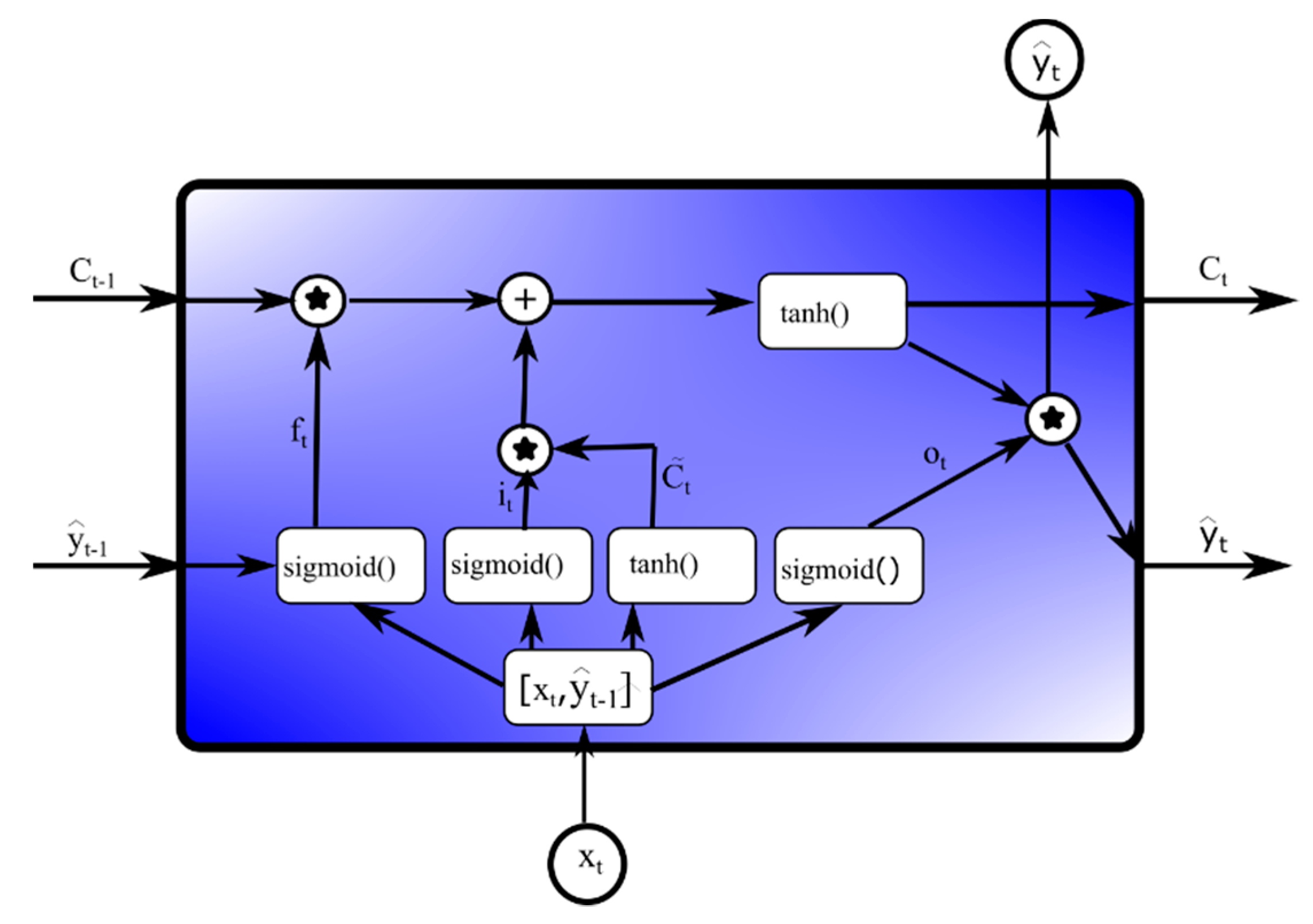
As mentioned above, LSTMs are a family of RNNs that are often used with deep neural networks. In summary, and as illustrated by Figure 2, an LSTM is made up of three gates: (1) a forget gate (f_t), which controls if/when the context is forgotten; (2) an input gate (i_t), which controls if/when a value should be remembered by the context; and (3) an output gate (o_t), which controls if/when the remembered value is allowed to pass from the unit. This exclusive structure of the LSTM is capable of effectively solving the problem of gradient loss and gradient explosion problems during the training procedure [23].
In a mathematical form, the above diagram (Figure 2) can be represented as follows:
f t = S ( W f · [ y ^ t 1 , x t ] + b f )
i t = S ( W i · [ y ^ t 1 , x t ] + b i )
C ˜ t = t a n h ( W C · [ y ^ t 1 , x t ] + b C )
C = f t · C t 1 + i t · C ^ t
o t = S ( W o · [ y ^ t 1 , x t ] + b o )
y ^ t = o t · t a n h ( C t )

2.6. Novel Hybrid Model Design

The use of the EWT to decompose data before use in the model is expected to improve the prediction accuracy and to solve the issue of long-term dependencies forecasting problems of the TCO monthly time series, such as the one used here. The EWT-LSTM developed here is also compared to the hybrid method based on the EMD and LSTM neural networks, namely EMD-LSTM. This hybrid model (EMD-LSTM) was applied to geophysical data for the first time by Zhang et al. [11]. The two above models are also compared to the LSTM model that uses wavelet denoised (WD) data (WD-LSTM), wavelet denoising EWT-LSTM (WD-EWT-LSTM), and wavelet denoising EMD-LSTM (WD-EMD-LSTM). For denoising, this study uses a Daubechies (db8) wavelet family in the PyWavelets Wavelet Transform software for Python. This family of wavelets is selected because it performed better than others in terms of applications in the forecasting of the TCO data. In addition, the LSTM system used here is a Python TensorFlow LSTM system that is run in miniconda [36].
Figure 3 illustrates the detailed procedures of the architecture of the hybrid model used in this study. Apart from the models that used the Wavelet denoising step, implementation of the EWT-LSTM and EMD-LSTM models developed here occurs in three important steps. The first step utilizes the EMD or EWT technique to decompose the TCO time series data into relatively stable IMFs and one residue item. In the second step, the LSTM neural network is used to forecast each normalized IMF, including the residue. In the third step, the forecasting results of the LSTM neural network are reverse-normalized before being accumulated through summation as the final predicted results. It is important to note that the TCO data were divided into 70% training and 30% testing datasets. The training dataset is used for the LSTM modeling, and the testing dataset is used as an input into the trained LSTM models to predict all the IMFs and the residue. After obtaining the final forecasting values, model performance evaluation is applied, utilizing several statistical metrics to assess the performance of all six models presented here.

2.7. Model Performance

In general, there is no standard criterion for assessing the forecasting performance of a model and comparison with other benchmark models [37]. In this study, the model performance evaluation is done by comparing the predicted values with their corresponding observed values using typical performance metrics, which are summarized in Table 1.

3. Results and Discussion

3.1. TCO Data Series and Trends

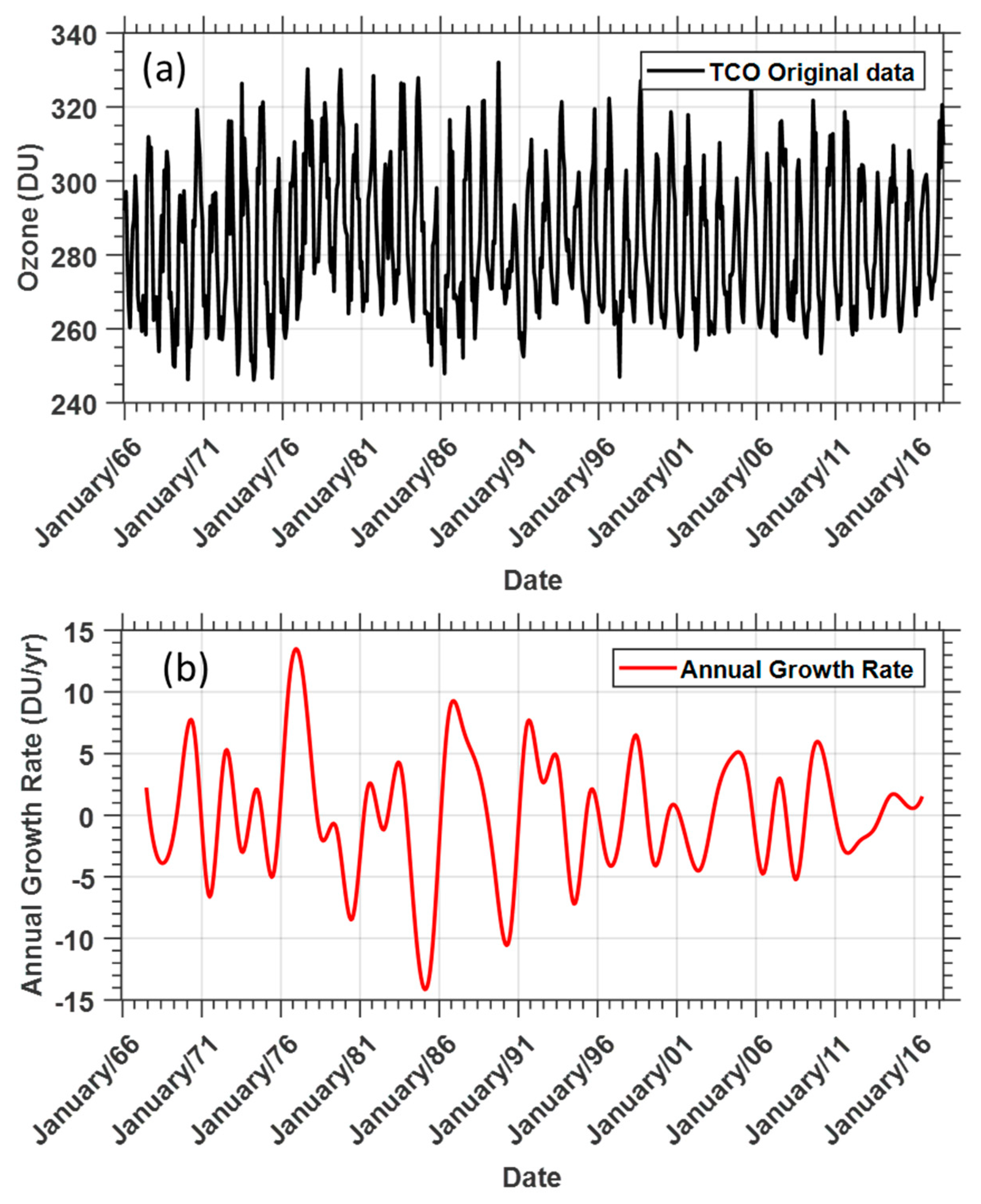
Figure 4a shows the monthly means of TCO time series measured at Observatorio Central Buenos Aires (OCBA) during the period 1966–2017. In general, the TCO time series over the study area indicates a strong seasonal variability, with maximum ozone during summer season and minimum values during winter.
Owing to the dynamics of the TCO especially in the Southern Hemisphere, it is also important to consider calculating the annual growth rate of the TCO data used here. This growth rate is defined as the instantaneous slope of the de-seasonalised curve. In this study, the annual growth rate was computed with the algorithm used by NOAA (National Oceanic and Atmosphere Administration), which was developed by Thoning et al. [38]. This method has been shown to be useful in extracting annual growth rates in a number of atmospheric chemistry climatology studies, including a recent study by Apadula et al. [39]. The method uses monthly mean TCO values corrected for the seasonal cycles, computes the averages of the four November, December, January, and February months every year, and associates these values to 1 January. The estimated value for the annual mean growth rate is then computed by evaluating the differences between the averages. Our study utilizes a twelve-month centered moving mean value for the OCBA TCO time series. The annual growth rate for the OCBA TCO time series is shown in Figure 4b.
In general, the mean growth rate for the OCBA TCO time series for the period from 1966 to 2017 is equal to 0.08 DU/year. An inspection of Figure 4b shows that the highest growth rate in the OCBA TCO data is obtained for the years 1976–1977 (13.5 DU/year) followed by 1988–1989 (8.6 DU/year). On the other hand, the lowest annual growth rate value was observed in 1987 (−14.1 DU/year). Overall, there was a strong variability of the TCO growth rate during the period between 1974 and 1984. The observed changes in the annual growth rate variability during the mid-nineties could be associated with the early successes of the Montreal Protocol implementation strategies, banning substances that depleted ozone. Moreover, this takes place at a similar time to when the upper stratospheric HCL, a proxy for stratospheric chlorine, started to decline from the early 2000s, as reported by Fioletov [40]. However, during this period, the annual growth rate recorded values above 5 DU/year during the 1997–1998, 2003, and 2009–2010 El Niño years, which is more likely the cause, As the El Niño-Southern Oscillation (ENSO) is known to influence TCO [41]. The National Aeronautics and Space Administration Ozone Watch [42] reported the year 1987 as one of the years that showed the greatest rate of ozone decrease as well as the longest persistence of the ozone hole in Southern Hemisphere. The growth rate time series presented in Figure 4b seems to be consistent with these findings because it experiences its highest minimum (−14 DU/year) during the year 1987. The observed growth rate minimas seem to coincide with ozone depletion events, resulting from some of the largest volcanic eruptions in the El Chichón in 1982 and Mount Pinatubo in 1991.
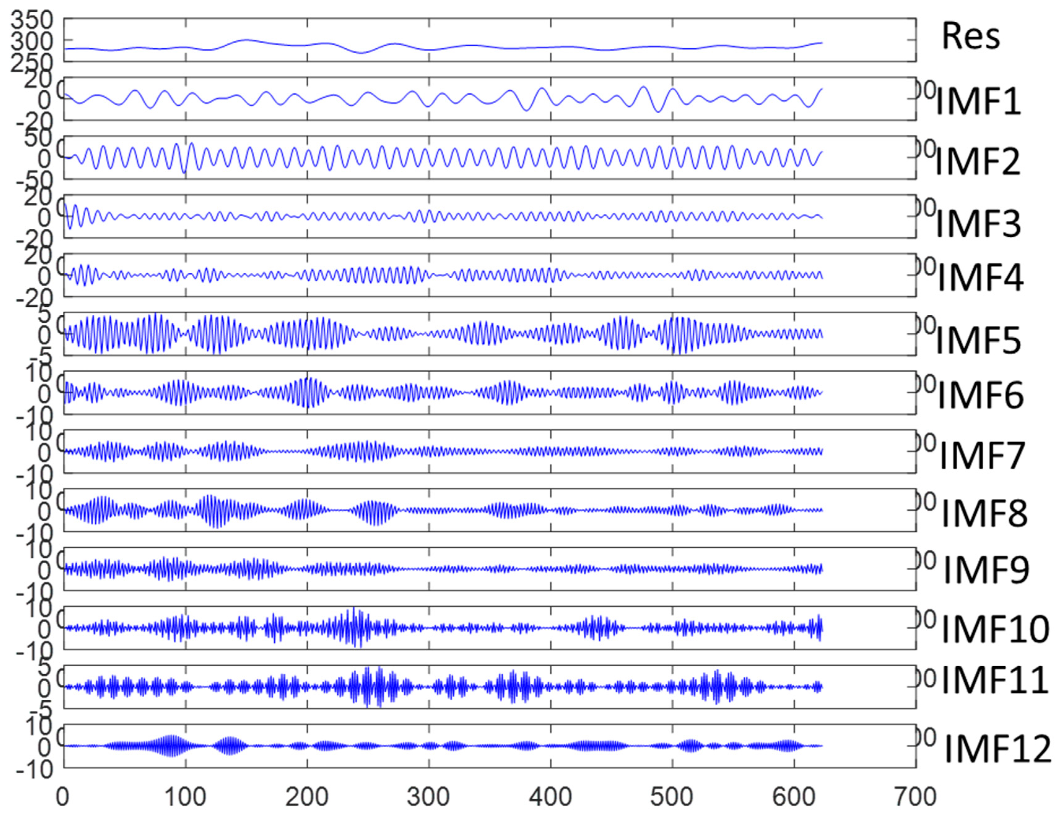
In this study, two powerful methods for conducting the decomposition of the non-stationary and non-linear signal are used, namely EMD and EWT. The decomposition of the time series is an integral part of the hybrid model for forecasting the TCO time series proposed here. The EMD method decomposed the original data series into seven relatively stable IMFs and one residue item (Figure 5). On the other hand, the EWT method was also applied to the original data series, and it produced twelve IMFs and one residue item (Figure 6). Generally, the IMFs extracted by both the EMD and EWT methods, indicate (1) the characteristics of lower and middle atmosphere time series data where the starting IMFs represent lower frequency and (2) the latter half IMFs indicate high frequencies, and (3) residuals are shown as trends. These characteristics indicate the presence of various periodicities such as solar cycle, QBO, annual cycle, and semi-annual cycle, among other periodicities. For the purpose of this study, the EMD amplitude of white noise was set to 0.2, and the ensemble number was set to 1000. In addition, all sub-band signals extracted by EMD and EWT were used in the decomposition step of the hybrid LSTM model.
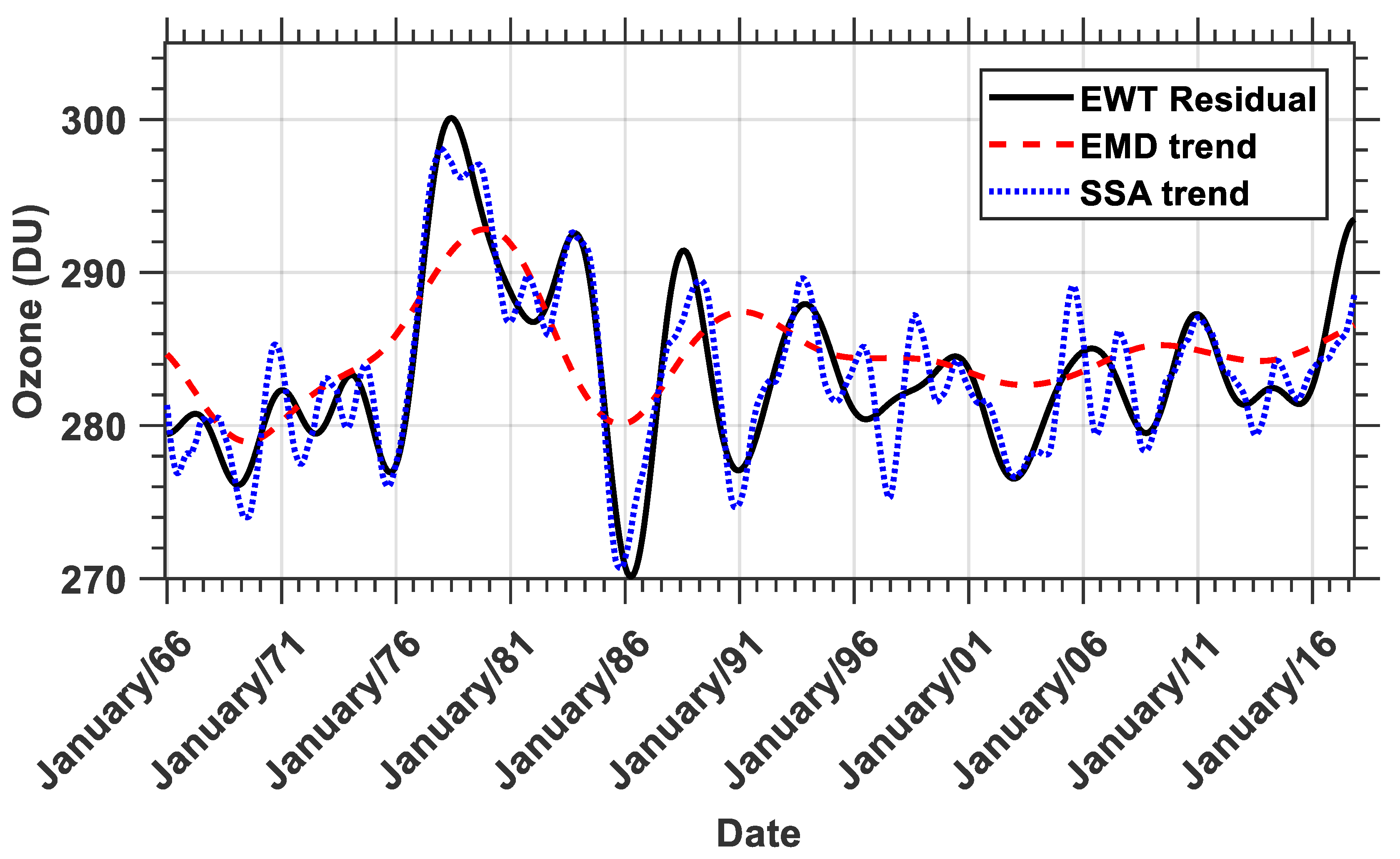
Generally, the limited availability of methods that have well-defined theory that can assist in the extraction of a trend in a time series poses a problem. The singular spectrum analysis (SSA) [43] trend extraction technique is a well-known method that captures the trend of a signal via eigenvalues from a trajectory matrix. Moreover, the EMD data-driven technique has been shown to offer the possibility of estimating a trend by summation of low-frequency intrinsic mode functions [44]. Previous studies have shown that EWT has an advantage over EMD, in addition to having a well-defined theory [22,45]. In our study, we successfully extracted the trend of the TCO time series (shown in Figure 4a) by means of the three above-mentioned methods (Figure 7). The EWT trend used here is the residue of the EWT, while the EMD trend was extracted via the summation of low-frequency intrinsic mode functions produced by the EMD [44]. Regarding the EMD, it is important to investigate whether each IMF (including the trend) is composed of useful information or just noise. Therefore, in this paper, we followed a method outlined by Wu and Huang [46], and also utilized features applied by Sang et al. [47] in their study of a comparison of the Mann-Kendal test and EMD method for trend identification in hydrological time series, in order to assess the statistical significance of EMD IMFs. These two trend analysis methods (EWT and EMD) are compared with the SSA trend method (Figure 7).
In Figure 7, it is apparent that the EWT residue is able to mimic the SSA trend very well. However, the SSA trend method is influenced by the 32- to 64-month periodicity, which is observed to be smoothened out in both the EWT and the EMD methods. Overall, the three methods used here are able to capture the disturbances of the TCO over Buenos Aires, which are associated with major events such as the 1987 major decline of ozone in the South Pole, as well as during some of the largest volcanic eruptions during the 1982 El Chichón and Mount Pinatubo during 1991. The observed TCO trend declines from the early 1980s before it becomes steady from the early 2000s onwards. The turning of the trend to an upwards direction is observed later in the time series, which indicates the effect of the Montreal Protocol. The Montreal Protocol and its subsequent amendments are known to have successfully prevented catastrophic losses of the stratospheric ozone [9].
In this study, we utilized several time series analysis techniques such as wavelet analysis, Mann-Kendall test, and sequential Mann-Kendall test model, and applied them to the Buenos Aires TCO data. The wavelet analysis technique was efficient in analyzing the localized variation of the spectral power within the OCBA TCO data. Overall, wavelet analysis is a common tool for this purpose and this signal processing method makes it possible to determine the dominant modes of variability, in addition to their variation within the time series. The annual Mann-Kendall trend test method was also performed by calculating annual z-score values throughout the time series. We found this non-parametric trend test method very suitable for the TCO trend analysis for two reasons: (1) it does not require the data to be normally distributed, and (2) it does not depend on the magnitude of the data. Furthermore, this method was supported by employing the sequential version of the Mann-Kendall test, in order to determine the change detection points in the OCBA TCO time series trend. Further details about the theory of the above mentioned time series analysis methods and their application can be found in a study by Mbatha et al. [28].
Figure 8 shows OCBA TCO monthly mean time series for the period from 1966 to 2017 with its smooth trend (a), normalized wavelet power spectra of the TCO data (b), annual mean Mann-Kendall calculated for TCO time series (c), and sequential Mann-Kendall statistics of progressive (Prog) u ( t ) and retrograde (Retr) u ( t ) (d). In the normalized wavelet power spectra in Figure 8b, the white thick lines represent the 95% confidence level, and areas of the wavelet power that are considered are those that are within the cone-of-influence (indicated by solid upside-down “u” shaped line). As expected, a strong peak at around the 12-month cycle dominates the wavelet power spectra of Buenos Aires TCO monthly mean time series. Apart from the dominant annual oscillation, we observe that there are prominent oscillations presented in the TCO time series, having periodicities of 16 to 18 months, 28 to 32 months (QBO periodicity), quasi 64 months, and evidence of a strong 11-year solar cycle.
The annual Mann-Kendall test time series shown in Figure 8c indicates distinctive periods of positive and significant z-score (greater than Z1 = 1.96), especially during major events, which are summarized in the TCO growth rate analysis in Figure 4. The positive significant z-score values seem to dominate in the period after the year 2000, with a similar period from 2014 to 2017, experiencing consistent positive z-score values. This is indicative of the effect of the Montreal Protocol agreement, and hence signs of the recovery of stratospheric ozone. This is also in agreement with the trends reported by SQ-MK in Figure 8d, indicating a downward trend for both the forward and backward (Prog and Retr) statistic values, having started in the 1970s and 1980s. Stabilization of this downward trend is observed from the beginning of the 2000s and later takes an upward (but not significant) direction in subsequent years. The specific change detection point is in the mid-2000s and during 2010.

3.2. Empirical Models Results and Its Performance

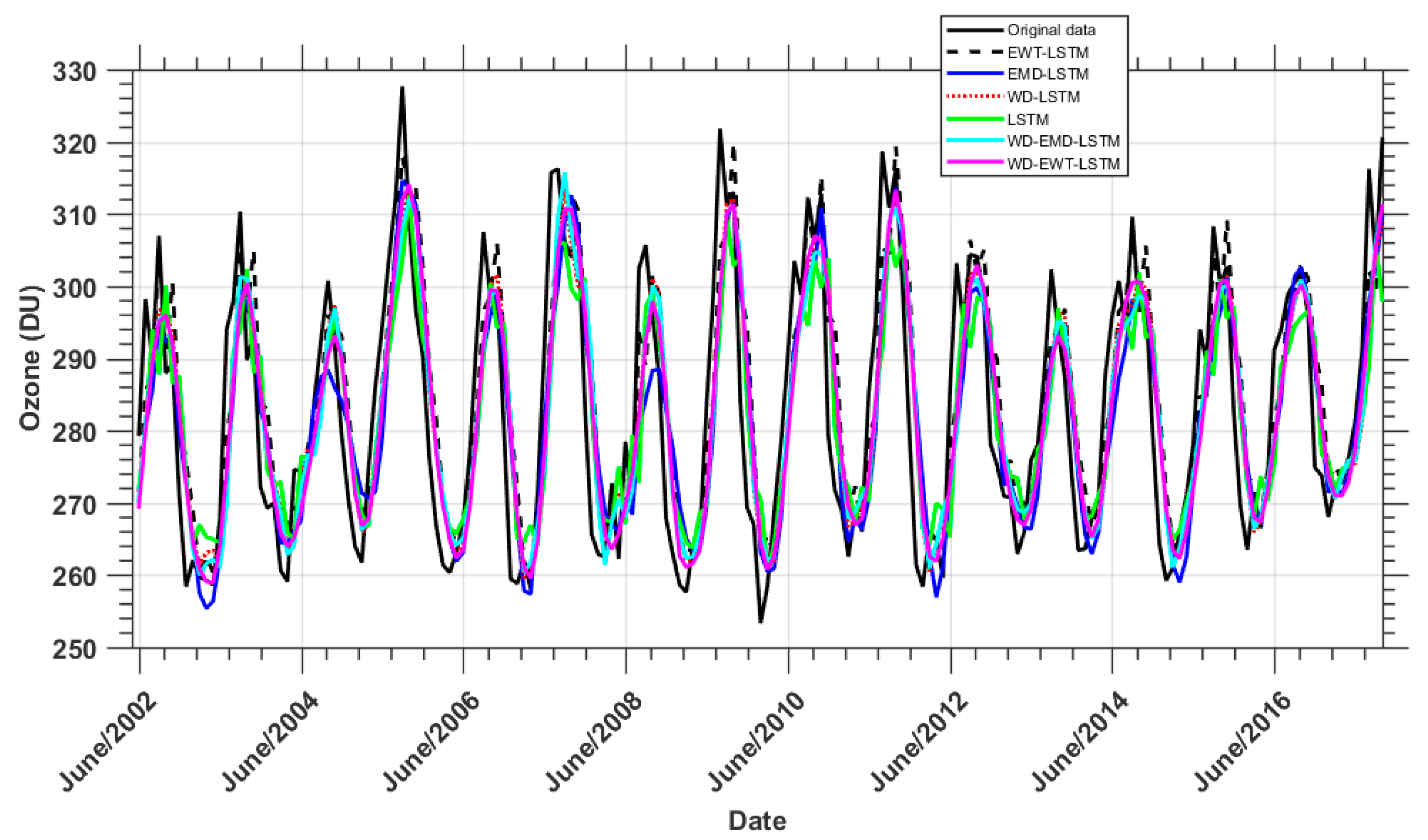
To improve the prediction accuracy of complex geophysical data from a simple time series model, one needs to consider taking advantage of signal preprocessing methods such as denoising, decomposition, and ensembling the predicted results. Therefore, to understand the performance of the hybrid EWT-LSTM model, the predicted results of the EWT-LSTM model are compared with the LSTM, EMD-LSTM, WD-LSTM, WD-EMD-LSTM, and WD-EWT-LSTM. In this study, the OCBA TCO time series is divided into 70% training part of the time series and the 30% testing part of the time series. Thus, the model was trained using data from January 1966 to May 2002, and the model forecast testing part of the time series started from 2002 to 2017. Figure 9 shows the predicted results of the six models plotted together with the original time series (testing time series). In this figure, it is apparent that the six models predict different forecast results of the TCO time series measured at the OCBA site. However, the hybrid EWT-LSTM, WD-EWT-LSTM, and EMD-LSTM models seem to perform better predictions compared with other ones. While it is difficult to comment on the other models, the single LSTM model is observed to hardly catch the sudden changes in the original time series. In order to further assess the prediction performance of the six models used here, a Taylor diagram [48] and statistical evaluation metrics such as MAE, MAPE, R, RMSE, and STD are utilized to measure the performance the models. The Taylor diagram is informative as it assists by visualization of the comparative strength of the models to the actual target variable. In the Taylor diagram, two different statistical metrics (i.e., correlation coefficients “R” and standard deviations “STD” of each model) are used to quantifying the comparability between the models and the observational data. The distance from the reference point, which is the observed data, is a measure of the cantered RMSE.
Figure 10 shows the Taylor diagram of the models used in this study. In this figure, owing to the denseness of the models, a zoomed view of the models position in the Taylor diagram is shown in the right panel of Figure 10. On the basis of the representation in Figure 10 for the six data-driven models used in this study, EWT-LSTM outperformed the other five models. The EWT-LSTM is the closest to the observed point, which means it has the smallest RMSE. EWT-LSTM also has the highest correlation of approximately R = 0.87, and the smallest standard deviation. The Taylor diagram also shows that time series preprocessing methods such as denoising and decomposition play a significant role in improving the accuracy of the model. This is because the LSTM model, a model that does not use preprocessed data, is the worst performing model in the view of the Taylor diagram.
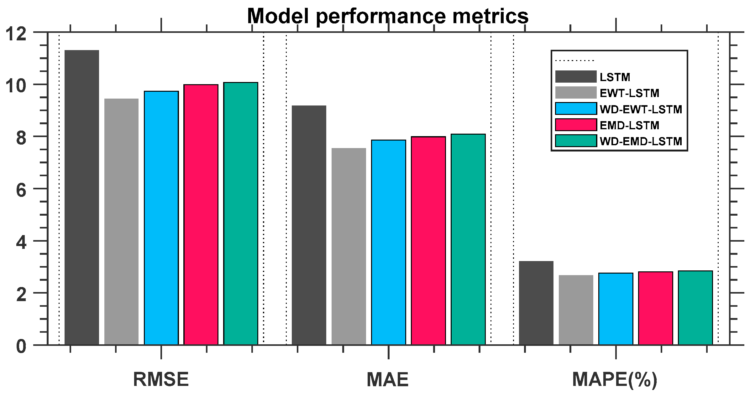
Figure 11 shows a bar graph that summaries the comparison of the model forecasting performance evaluated using three criteria, namely, RMSE, MAE, and MAPE. A visual inspection of Figure 9 and the Taylor diagram in Figure 10 seems to indicate the existence of a preliminary judgment that the forecasting accuracy of the EWT-LSTM model is higher than that of the other five models proposed in this study. Moreover, it can be observed in Figure 11 that, among all the forecasting models used here, EWT-LSTM performs better than any other model, namely, LSTM, WD-EWT-LSTM, EMD, and WD-EMD-LSTM, in terms of RMSE, MAE, and MAPE, which are 9.4, 7.5, and 2.6%, respectively. The LSTM model, a model that does not consider any of the data preprocessing methods used in this study, is the worst performing model. The aforementioned is presumably owing to the non-stationary and non-linear nature of the original monthly mean TCO data series, which is captured by the preprocessing methods used here. On the other hand, preprocessing of data with methods such as denoising and decomposition is known to improve the performance of the LSTM model and other artificial neural network models [11,14,17]. The use of the wavelet transform denoising technique, a model design reported for the first time in this study, seems to improve the LSTM model accuracy. Better model accuracy is obtained when the model’s original data are decomposed using EMD [11] or EWT. However, denoising the data before decomposing and then applying the LSTM neural network on it does not improve the model. This is because LSTM is able to learn both long-term and short-term variation in the data, which also accommodates some level of noise in the data. Moreover, it is possible that the denoising step also removes some important pattern in the data across time. Generally, EWT, a new method to detect the principal “modes” that represent the signal, and with good mathematical theory, seems to perform better than the popular EMD method, which lacks mathematical theory when applied in the decomposition step of the model.

4. Conclusions

The present study utilized different time series analysis methods to investigate the trend and variability of the TCO monthly mean time series, in addition to developing and testing six LSTM recurrent neural networks based data-driven time series forecasting models. The TCO data, long-term ozone data measured at the Buenos Aires site, Argentina, from 1966 to 2017, were used in this study. Overall, the trends of TCO time series data extracted using the SSA, EWT, EMD, and Mann-Kendall confirm that the TCO has been stable since the mid-1990s. The SSA growth rate and trend, EMD trend, and EWT trend capture the dynamical variability of the TCO well, and their results are somewhat consistent. All trend analysis methods seem to report a significant recovery of ozone during the period from 2010 to 2017, apart from the decline of ozone observed during 2015, which is presumably associated with the Calbuco volcanic event (a Chilean volcano that has injected volcanic plume up to the stratosphere, as reported by Bègue et al. [49,50]). The sensitivity of the EWT trend results presented in Figure 7 seems to indicate that the EWT extraction method, a method that has a well-defined mathematical theory compared with others, can be the best method for trend extraction.
Six LSTM neural networks based data-driven time series forecasting models, namely, LSTM, EWT-LSTM, EMD-LSTM, WD-LSTM, WD-EWT-LSTM, and WD-EMD-LSTM, were developed in this research. The mode that used the EWT decomposition process (EWT-LSTM) outperformed the other five models in terms of forecasting performance evaluation criteria, such as the RMSE, MAE, MAPE, and R. In general, better model accuracy was achieved for those models that used decomposition methods, demonstrating that EMD and EWT methods play a significant role in the improvement of the performance of the LSTM model. Noise reduction techniques via wavelet transform improved the LSTM model accuracy, but it appears unnecessary to denoise data to the data when utilizing the decomposition process. Overall, the results presented in this study show that the EWT-LSTM model can be used as a successful tool for monthly mean TCO forecasting.
For future work, it is recommended to use a method that has good mathematical theory such as the EWT technique to perform trend analysis of ozone data, or any other geophysical time series. The continuation of this study will include applying the techniques developed to the stratospheric column ozone, lower stratosphere ozone, and upper stratosphere ozone measured in the high latitude Southern Hemisphere, in order to forecast the process of ozone hole recovery. Additionally, more TCO measuring sites at different latitudes will also be considered in future studies.

Author Contributions

Conceptualization, N.M. and H.B.; methodology, N.M.; software, N.M.; validation, N.M.; formal analysis, N.M.; investigation, N.M. and H.B.; writing—original draft preparation, N.M. and H.B.; writing—review and editing, N.M. and H.B.; visualization, N.M. All authors have read and agreed to the published version of the manuscript.

Funding

This research was funded jointly by the CNRS (Centre National de la Recherche Scientifique) and the NRF (National Research Foundation) in the framework of the LIA ARSAIO and by the South Africa/France PROTEA Program (project No 42470VA).

Acknowledgments

Authors acknowledge the French South-African PROTEA programme and the CNRS-NRF LIA ARSAIO (Atmospheric Research in Southern Africa and Indian Ocean), for supporting research activities, and the National Research Foundation (NRF) of South Africa. We are thankful to the World Ozone and Ultraviolet Radiation Data Centre (WOUDC) for data archiving, the PI and operators of Dobson instrument at Buenos Aires, and the National Meteorological Service of Argentina (SMNA).

Conflicts of Interest

The authors declare no conflict of interest.

References

  1. Weber, M.; Coldewey-Egbers, M.; Fioletov, V.E.; Frith, S.M.; Wild, J.D.; Burrows, J.P.; Long, C.S.; Loyola, D. Total ozone trends from 1979 to 2016 derived from five merged observational datasets – the emergence into ozone recovery. Atmos. Chem. Phys. 2018, 18, 2097–2117. [Google Scholar] [CrossRef] [Green Version]
  2. Farman, J.C.; Gardiner, B.G.; Shanklin, J.D. Large losses of total ozone in Antarctica reveal seasonal ClO x/NO x interaction. Nature 1985, 315, 207–210. [Google Scholar] [CrossRef]
  3. Solomon, S.; Garcia, R.R.; Rowland, F.S.; Wuebbles, D.J. On the depletion of Antarctic ozone. Nature 1986, 321, 755–758. [Google Scholar] [CrossRef] [Green Version]
  4. Rigby, M.; Park, S.; Saito, T.; Western, L.M.; Redington, A.L.; Fang, X.; Henne, S.; Manning, A.J.; Prinn, R.G.; Dutton, G.S. Increase in CFC-11 emissions from eastern China based on atmospheric observations. Nature 2019, 569, 546–550. [Google Scholar] [CrossRef] [PubMed]
  5. Ball, W.T.; Alsing, J.; Mortlock, D.J.; Staehelin, J.; Haigh, J.D.; Peter, T.; Tummon, F.; Stübi, R.; Stenke, A.; Anderson, J.; et al. Evidence for a continuous decline in lower stratospheric ozone offsetting ozone layer recovery. Atmos. Chem. Phys. 2018, 18, 1379–1394. [Google Scholar] [CrossRef] [Green Version]
  6. Braesicke, P.; Neu, J.; Fioletov, V.; Godin-Beekmann, S.; Hubert, D.; Petropavlovskikh, I.; Shiotani, M.; Sinnhuber, B.-M. Update on Global Ozone: Past, Present, and Future. In Scientific Assessment of Ozone Depletion: 2018; Global Ozone Research and Monitoring Project–Report No. 58; World Meteorological Organization: Geneva, Switzerland, 2018; Chapter 3. [Google Scholar]
  7. Pawson, S.; Steinbrecht, W.; Charlton-Perez, A.J.; Fujiwara, M.; Karpechko, A.Y.; Petropavlovskikh, I.; Urban, J.; Weber, M.; Aquila, V.; Chehade, W. Update on global ozone: Past, present, and future. In Scientific Assessment of Ozone Depletion: 2014; Global Ozone Research and Monitoring Project–Report No. 55; World Meteorological Organization: Geneva, Switzerland, 2014; Chapter 3. [Google Scholar]
  8. Chehade, W.; Weber, M.; Burrows, J.P. Total ozone trends and variability during 1979–2012 from merged data sets of various satellites. Atmos. Chem. Phys. 2014, 14, 7059–7074. [Google Scholar] [CrossRef] [Green Version]
  9. Ball, W.T.; Alsing, J.; Staehelin, J.; Davis, S.M.; Froidevaux, L.; Peter, T. Stratospheric ozone trends for 1985–2018: Sensitivity to recent large variability. Atmos. Chem. Phys. 2019, 19, 12731–12748. [Google Scholar] [CrossRef] [Green Version]
  10. Lei, M.; Shiyan, L.; Chuanwen, J.; Hongling, L.; Yan, Z. A review on the forecasting of wind speed and generated power. Renew. Sust. Energ. Rev. 2009, 13, 915–920. [Google Scholar] [CrossRef]
  11. Zhang, X.; Zhang, Q.; Zhang, G.; Nie, Z.; Gui, Z.; Que, H. A Novel Hybrid Data-Driven Model for Daily Land Surface Temperature Forecasting Using Long Short-Term Memory Neural Network Based on Ensemble Empirical Mode Decomposition. Int. J. Environ. Res. Public. Health. 2018, 15, 1032. [Google Scholar] [CrossRef] [Green Version]
  12. Zhang, G.P.; Qi, M. Neural network forecasting for seasonal and trend time series. Eur. J. Oper. Res. 2005, 160, 501–514. [Google Scholar] [CrossRef]
  13. Tealab, A. Time series forecasting using artificial neural networks methodologies: A systematic review. future computing inform. j. 2018, 3, 334–340. [Google Scholar] [CrossRef]
  14. Tian, C.; Hao, Y.; Hu, J. A novel wind speed forecasting system based on hybrid data preprocessing and multi-objective optimization. Applied Energy 2018, 231, 301–319. [Google Scholar] [CrossRef]
  15. Zhang, G.P. Time series forecasting using a hybrid ARIMA and neural network model. Neurocomputing 2003, 50, 159–175. [Google Scholar] [CrossRef]
  16. Khandelwal, I.; Adhikari, R.; Verma, G. Time Series Forecasting Using Hybrid ARIMA and ANN Models Based on DWT Decomposition. Procedia Comput. Sci. 2015, 48, 173–179. [Google Scholar] [CrossRef] [Green Version]
  17. Zhou, J.; Peng, T.; Zhang, C.; Sun, N. Data Pre-Analysis and Ensemble of Various Artificial Neural Networks for Monthly Streamflow Forecasting. Water 2018, 10, 628. [Google Scholar] [CrossRef] [Green Version]
  18. Altan, A.; Karasu, S.; Bekiros, S. Digital currency forecasting with chaotic meta-heuristic bio-inspired signal processing techniques. Chaos Soliton. Fract. 2019, 126, 325–336. [Google Scholar] [CrossRef]
  19. Liu, Y.; Guan, L.; Hou, C.; Han, H.; Liu, Z.; Sun, Y.; Zheng, M. Wind Power Short-Term Prediction Based on LSTM and Discrete Wavelet Transform. Appl. Sci. 2019, 9, 1108. [Google Scholar] [CrossRef] [Green Version]
  20. Li, Y.; Wu, H.; Liu, H. Multi-step wind speed forecasting using EWT decomposition, LSTM principal computing, RELM subordinate computing and IEWT reconstruction. Energy Convers. Manag. 2018, 167, 203–219. [Google Scholar] [CrossRef]
  21. Nazir, H.M.; Hussain, I.; Faisal, M.; Shoukry, A.M.; Gani, S.; Ahmad, I. Development of Multidecomposition Hybrid Model for Hydrological Time Series Analysis. Complexity 2019, 2019, 1–14. [Google Scholar] [CrossRef]
  22. Gilles, J. Empirical wavelet transform. IEEE Trans. Signal. Process. 2013, 61, 3999–4010. [Google Scholar] [CrossRef]
  23. Hochreiter, S.; Schmidhuber, J. Long Short-Term Memory. Neural Computation 1997, 9, 1735–1780. [Google Scholar] [CrossRef] [PubMed]
  24. World Ozone and Ultraviolet Radiation Data Centre website. Available online: https://woudc.org/home.php (accessed on 30 June 2018).
  25. Dobson, G.M.B.; Harrison, D.N.; Lindemann, F.A. Measurements of the amount of ozone in the earth’s atmosphere and its relation to other geophysical conditions. P. R. Soc. A-Math. Phy. 1926, 110, 660–693. [Google Scholar] [CrossRef]
  26. Stolarki, R.S.; Krueger, A.J.; Schoeberl, M.R.; McPeters, R.D.; Newman, P.A.; Alpert, J.C. Nimbus 7 SBUV/TOMS measurements of the springtime Antarctic ozone hole. Nature 1986, 322, 808–811. [Google Scholar] [CrossRef]
  27. Grant, W.B. Ozone Measuring Instruments for the Stratosphere; Collection Work in Optics; Optical Society of Amer: Washington DC, USA, 1989. [Google Scholar]
  28. Mbatha, N.; Xulu, S. Time Series Analysis of MODIS-Derived NDVI for the Hluhluwe-Imfolozi Park, South Africa: Impact of Recent Intense Drought. Climate 2018, 6, 95. [Google Scholar] [CrossRef] [Green Version]
  29. Mann, H.B. Nonparametric tests against trend. Econometrica. 1945, 13, 245–259. [Google Scholar] [CrossRef]
  30. Sneyers, R. On the statistical analysis of series of observations; Technical Note 143; World Metrological Organization, : Geneva, Switzerland, 1991. [Google Scholar]
  31. Pohlert, T. Trend: Non-Parametric Trend Tests and Change-Point Detection. Available online: https://cran.r-project.org/web/packages/trend/index.html (accessed on 6 August 2018).
  32. Schaber, J. Pheno: Auxiliary Functions for Phenological Data Analysis. Available online: https://cran.r-project.org/web/packages/pheno/index.html (accessed on 6 August 2018).
  33. Torres, M.E.; Colominas, M.A.; Schlotthauer, G.; Flandrin, P. A complete ensemble empirical mode decomposition with adaptive noise. In Proceedings of the 2011 IEEE International Conference on Acoustics, Speech and Signal Processing (ICASSP), Prague, Czech Republic, 22–27 May 2011; pp. 4144–4147. [Google Scholar]
  34. Daubechies, I. Ten Lectures on Wavelets; SIAM: Bangkok, Thailand, 1992. [Google Scholar]
  35. Giles, C.L.; Lawrence, S.; Tsoi, A.C. Noisy Time Series Prediction using Recurrent Neural Networks and Grammatical Inference. Mach. Learn. 2001, 44, 161–183. [Google Scholar] [CrossRef] [Green Version]
  36. Miniconda—Conda documentation. Available online: https://docs.conda.io/en/latest/miniconda.html (accessed on 1 May 2019).
  37. Xu, Y.; Yang, W.; Wang, J. Air quality early-warning system for cities in China. Atmos. Environ. 2017, 148, 239–257. [Google Scholar] [CrossRef]
  38. Thoning, K.W.; Tans, P.P.; Komhyr, W.D. Atmospheric carbon dioxide at Mauna Loa Observatory: 2. Analysis of the NOAA GMCC data, 1974–1985. J. Geophys. Res: Atmos. 1989, 94, 8549–8565. [Google Scholar] [CrossRef]
  39. Apadula, F.; Cassardo, C.; Ferrarese, S.; Heltai, D.; Lanza, A. Thirty Years of Atmospheric CO2 Observations at the Plateau Rosa Station, Italy. Atmosphere 2019, 10, 418. [Google Scholar] [CrossRef] [Green Version]
  40. Fioletov, V.E. Ozone climatology, trends, and substances that control ozone. Atmos. Ocean. 2008, 46, 39–67. [Google Scholar] [CrossRef] [Green Version]
  41. Toihir, A.M.; Portafaix, T.; Sivakumar, V.; Bencherif, H.; Pazmino, A.; Bègue, N. Variability and trend in ozone over the southern tropics and subtropics. Ann. Geophys. 2018, 36, 381–404. [Google Scholar] [CrossRef] [Green Version]
  42. NASA Ozone Watch: Latest status of ozone. Available online: https://ozonewatch.gsfc.nasa.gov/ (accessed on 2 February 2020).
  43. Harmouche, J.; Fourer, D.; Auger, F.; Borgnat, P.; Flandrin, P. The sliding singular spectrum analysis: A data-driven nonstationary signal decomposition tool. IEEE Trans. Signal. Process. 2017, 66, 251–263. [Google Scholar] [CrossRef] [Green Version]
  44. Moghtaderi, A.; Borgnat, P.; Flandrin, P. Trend filtering: Empirical mode decompositions versus ℓ1 and Hodrick–Prescott. Adv. Adapt. Data Anal. 2011, 3, 41–61. [Google Scholar] [CrossRef]
  45. Geetikaverma, V.S. Empirical Wavelet Transform & its Comparison with Empirical Mode Decomposition: A review. Int. J. Appl. Eng. 2016, 4, 5. [Google Scholar]
  46. Wu, Z.; Huang, N.E. A study of the characteristics of white noise using the empirical mode decomposition method. P. R. Soc. A-Math. Phy. 2004, 460, 1597–1611. [Google Scholar] [CrossRef]
  47. Sang, Y.-F.; Wang, Z.; Liu, C. Comparison of the MK test and EMD method for trend identification in hydrological time series. J. Hydrol. 2014, 510, 293–298. [Google Scholar] [CrossRef]
  48. Taylor, K.E. Summarizing multiple aspects of model performance in a single diagram. J. Geophys. Res. Atmos. 2001, 106, 7183–7192. [Google Scholar] [CrossRef]
  49. Bègue, N.; Vignelles, D.; Berthet, G.; Portafaix, T.; Payen, G.; Jégou, F.; Benchérif, H.; Jumelet, J.; Vernier, J.-P.; Lurton, T.; et al. Long-range transport of stratospheric aerosols in the Southern Hemisphere following the 2015 Calbuco eruption. Atmos. Chem. Phys. 2017, 17, 15019–15036. [Google Scholar] [CrossRef] [Green Version]
  50. Bègue, N.; Shikwambana, L.; Bencherif, H.; Pallotta, J.; Sivakumar, V.; Wolfram, E.; Mbatha, N.; Orte, F.; Du Preez, J.; Ranaivombola, M.; et al. Statistical analysis of the long-range transport of the 2015 Calbuco volcanic eruption from ground-based and space-borne observations. Ann. Geophys. 2020, 38, 395–420. [Google Scholar]
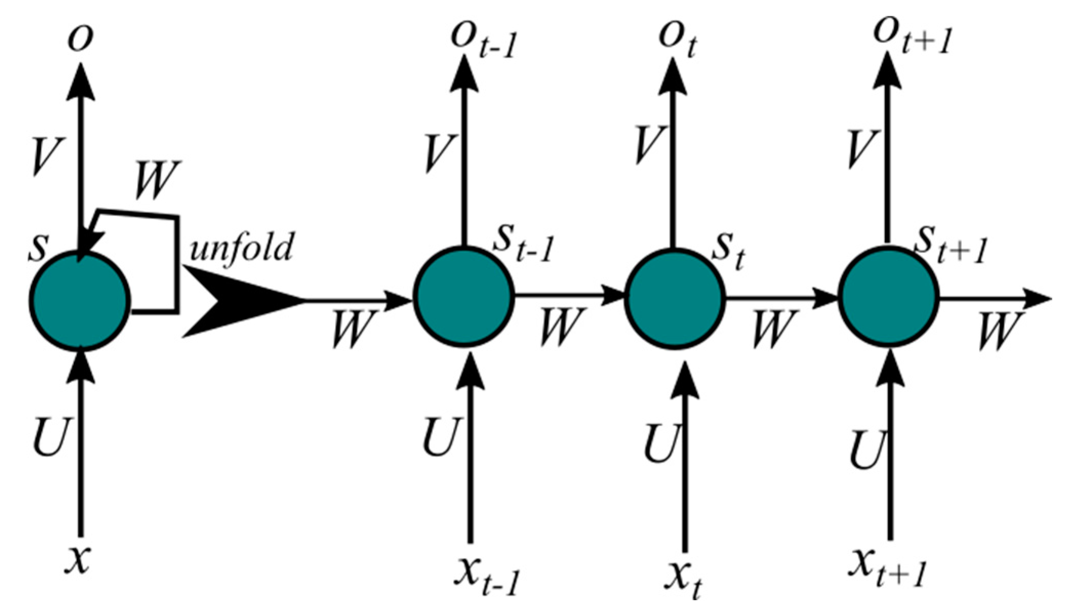
Figure 1. Architecture of a recurrent neural network (RNN).
Atmosphere 11 00457 g001
Figure 2. The structure of the long short-term memory (LSTM) unit.
Atmosphere 11 00457 g002
Figure 3. The architecture of the data driven LSTM hybrid model. IMF, intrinsic mode function; EWT, empirical wavelet transform; EMD, empirical mode decomposition.
Atmosphere 11 00457 g003
Figure 4. Total columns of ozone (TCO) time series at the Observatorio Central Buenos Aires (OCBA) (a) and its corresponding annual mean growth rate (b).
Atmosphere 11 00457 g004
Figure 5. Modes extracted by empirical mode decomposition (EMD) for OCBA TOC ozone time series.
Atmosphere 11 00457 g005
Figure 6. Modes extracted by empirical wavelet transform (EWT) for OCBA TCO ozone time series.
Atmosphere 11 00457 g006
Figure 7. OCBA TCO trend time series extracted by (EWT) (black line), EMD (red dashed line), and singular spectrum analysis (SSA) (blue dotted line).
Atmosphere 11 00457 g007
Figure 8. OCBA TCO time series with its smooth trend (a), normalized wavelet power spectra of the TCO data (b), annual mean Mann-Kendall calculated for TCO (c), and sequential Mann-Kendall statistics values (d).
Atmosphere 11 00457 g008
Figure 9. Forecasting results of the OCBA TCO time series for the period of June 2002 to December 2017 as derived by the use of six models (LSTM, EWT-LSTM, EMD-LSTM, wavelet denoising (WD)-LSTM, WD-EWT-LSTM, and WD-EMD-LSTM) together with the TCO monthly mean values derived from observations (original data).
Atmosphere 11 00457 g009
Figure 10. Taylor diagram graphical representation of six predictive models developed for forecasting OCBA TCO time series from 2002 to 2017.
Atmosphere 11 00457 g010
Figure 11. Error graphics of models performance of OCBA TCO time series. RMSE, root mean square error; MAE, mean absolute error; MAPE, mean absolute percentage error.
Atmosphere 11 00457 g011
Table 1. Model performance metrics.
MetricDefinitionFormula
MAEMean absolute error M A E = 1 N j = 1 N | p e s t i m a t e d j p r e a l j |
RMSERoot mean square error R M S E = 1 N j = 1 N ( p e s t i m a t e d j p r e a l j ) 2
MAPEMean absolute percentage error M A P E = 1 N j = 1 N | p e s t i m a t e d j p r e a l j p r e a l i |