Article

Thermal Inversion and Particulate Matter Concentration in Wrocław in Winter Season

by
Jadwiga Nidzgorska-Lencewicz
* and
Małgorzata Czarnecka
Department of Environmental Management, West Pomeranian University of Technology in Szczecin, ul. Papieża Pawła VI, 71-459 Szczecin, Poland
*
Author to whom correspondence should be addressed.
Atmosphere 2020, 11(12), 1351; https://doi.org/10.3390/atmos11121351
Submission received: 15 October 2020 / Revised: 3 December 2020 / Accepted: 7 December 2020 / Published: 12 December 2020
(This article belongs to the Special Issue Particulate Matters Emission in Poland)

Abstract

:
Studies on air quality frequently adopt clustering, in particular the k-means technique, owing to its simplicity, ease of implementation and efficiency. The aim of the present paper was the assessment of air quality in a winter season (December–February) in the conditions of temperature inversion using the k-means method, representing a non-hierarchical algorithm of cluster analysis. The air quality was assessed on the basis of the concentrations of particulate matter (PM10, PM2.5). The studies were conducted in four winter seasons (2015/16, 2016/17, 2017/18, 2019/20) in Wrocław (Poland). As a result of the application of the v-fold cross test, six clusters for each fraction of PM were identified. Even though the analysis covers only four winter seasons, the applied method has unequivocally revealed that the characteristics of surface-based (SBI) and elevated inversions (ELI) affect the concentration level of both fractions of particulate matter. In the case of PM10, the average lowest daily concentration (15.5 µg·m−3) was recorded in the conditions of approx. 205 m in thickness, 0.5 °C intensity of the SBI and at the height of the base of the ELI at approx. 1700 m a.g.l., a thickness of 148 m and an intensity of 1.2 °C. In turn, the average highest concentration (136 µg·m−3) was recorded at a thickness of SBI of approx. 400 m and an intensity of 1.4 °C. Such high concentration occurred when the lowest location of ELI formed at 764 m a.g.l. with a thickness of 308 m and an intensity of 0.96 °C. A marked role of the thickness of the SBI and ELI as well as the height of the base of the lowest location of ELI was also manifested with respect to PM2.5 concentrations.

1. Introduction

Temperature inversions (TI) are natural phenomena usually defined as layers in the atmosphere, across which the temperature increases with height. Temperature inversions form as a result of natural processes determining the climate and develop, mostly, due to radiative cooling of the Earth’s surface and adjacent air layers, warm advection above a relatively colder air mass or surface, and air subsidence [1,2,3,4]. The tropospheric TI plays an essential role in further shaping the weather and climate, determining atmospheric stability, and reducing or completely inhibiting the transfer of heat and moisture within the atmosphere [5,6]. Given the vertical extent of the phenomenon, the following are distinguished: surface-based inversions (SBI), and elevated inversions (ELI) present in the free atmosphere. However, most of the studies on the topic are restricted to the surface inversions or the first elevated inversions only [2,3,4,7,8]. Inversions occur in all climate zones, but their frequency shows high spatial variability. In the literature on the subject, apart from recognising the phenomena [1,2,3,4,9] often in terms of climate change, TI are mostly discussed with respect to higher latitudes where conditions are most favourable for their formation [5,6,10].
In recent years, there have been numerous studies discussing TI with respect to air quality. Conditions favourable to or limiting vertical mixing of polluted air are closely connected with the thermal stratification of the lower troposphere. TI in the lower atmosphere creates stable atmospheric conditions inhibiting vertical movement which can play a crucial role in the accumulation of air pollution. Numerous publications discussing seasons or winter episodes of elevated concentration of pollutants pointed to inversion layers present in the lower part of the troposphere as one of the causative factors [11,12,13,14,15,16].
The present paper discusses air quality relating to the occurrence of TI. Air quality is reflected by particulate matter concentration (PM)—specifically, its two most frequently measured fractions, i.e., PM10 and PM2.5. The literature on the subject defines PM as a complex mixture of different chemical components including water soluble ions, trace metals and organic compounds that emerge from a wide range of natural and anthropogenic sources [17,18,19]. Selecting PM for the present analysis is deliberate, since despite the recently observed marked improvements in air quality, excess particulate matter concentration is still being recorded in most cities worldwide, as is its negative effect on human health, even at relatively low mass concentrations [20,21,22,23]. According to the estimates of the Organisation for Economic Co-operation and Development (OECD), only 2% of the global urban population is living in areas where PM10 concentrations are lower than that stipulated by World Health Organisation (WHO) in air quality guidelines [24]. In Poland, just as in many other countries of Central and Central-Eastern Europe, very high PM concentrations are recorded every winter season. This is due to the still high share of solid fuels in the primary energy source structure and large share of low communal emission. PM emissions in Poland are among the highest in the European Union—in 2013, PM10 amounted to 12.6% and PM2.5 to 10.9% of the total emissions [25].

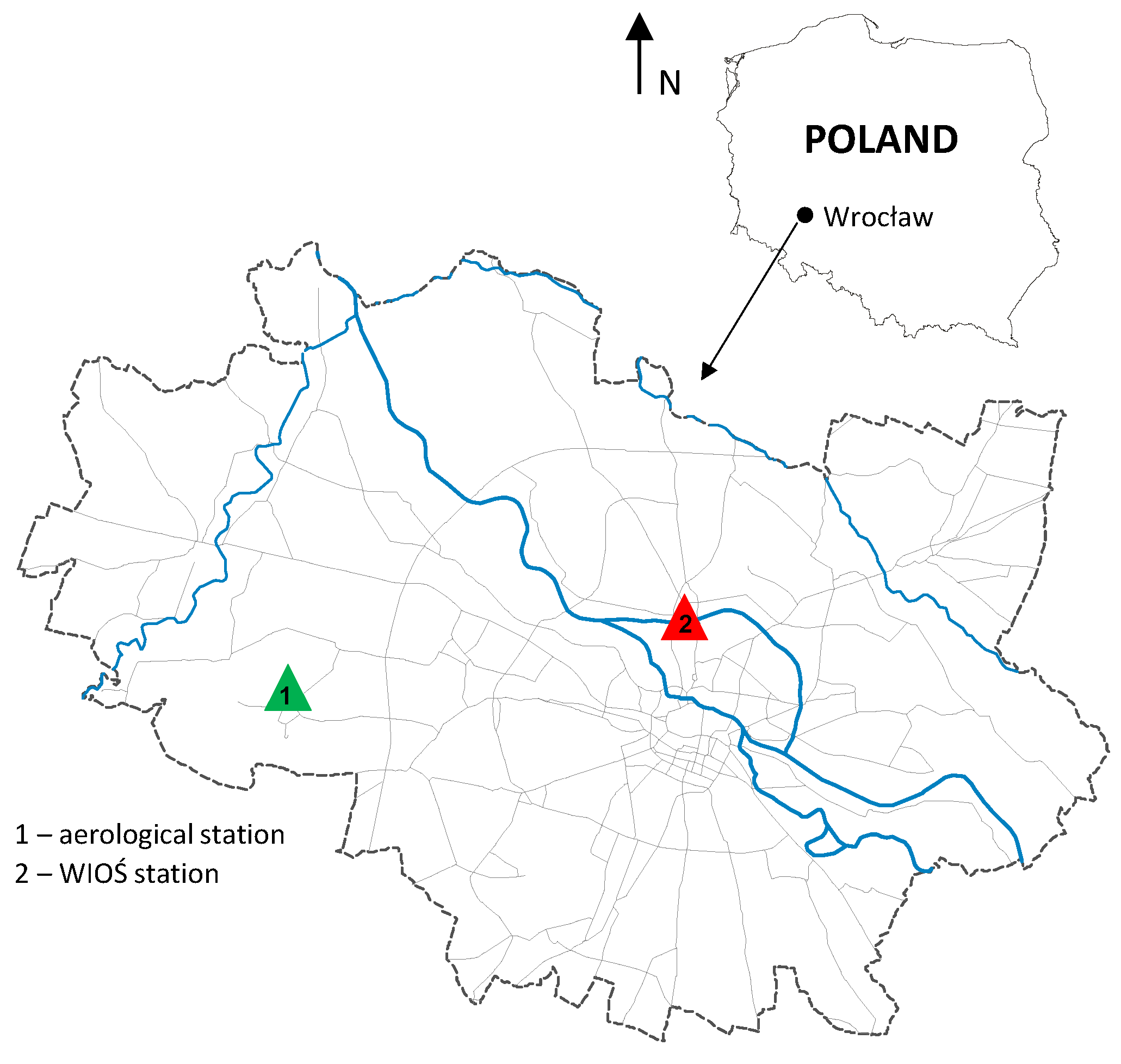
2. Materials and Methods

The study was based on the results of the radiosounding measurements conducted at Hydrological and Meteorological Station IMGW-PIB in Wrocław (No. WMO: 12425) taken at 00 UTC and 12 UTC during the calendar winter period (DJF) in the years 2015–2020, available at [26]. In the analysed period, measurements were taken using the survey systems DigiCORA Vaisala radiosondes RS92SGPD, RS92SGPD and RS41SG( Vaisala Corporation, Helsinki, Finland). Owing to the lack of aerological measurements from 22 December 2018 to 12 March 2019, the study included 4 winter seasons (without the winter season of 2018/19). The analysis of the vertical profiles of air temperature in 362 days of the four winter seasons, separate for night-time (00.00 UTC) and daytime (12.00 UTC), allowed for the determination of SBI and ELI. The methodology of identifying the inversion layers on the basis of the radiosounding results is presented in detail in our previous study [2]. With respect to SBI, the thickness was determined, while for ELI, the altitude of the base and thickness were identified. The characteristics of both types of inversion take into consideration their strength (in °C per 100 m). The thickness of SBI and ELI were equivalent to the thickness of the layer with a positive vertical temperature gradient. With respect to SBI, the said layer extended directly from the ground level to an altitude above which air temperature demonstrated a decrease with height. On several occasions, it was found that in the atmosphere (especially over urban and industrial areas), there were many ELI layers that were separated by layers of air when the temperature decreased with altitude; therefore, this study takes into consideration only the lowermost ELI. The available, relatively scarce, literature on inversion includes numerous and diverse methods of identifying the phenomenon. In the characteristics of the occurrence of thermal blocking layers in Poland, Parczewski [27] identified inversions, isotherms and layers of slight (≤0.20 °C over 100 m) temperature gradient present up to the altitude of 1000 m. In line with the results by Knozová [7] for Prague, the present paper adopted the first layer of elevated inversion as the layer with the base at the altitude of no more than 3000 m.
The concentrations of PM10 and PM2.5 were recorded from Wrocław station—Korzeniowskiego (national code—DsWrocWybCon, international—PL0194A), operated by the Regional Inspectorate for Environmental Protection (WIOŚ) in Wrocław, available at [28]. The location of the aerological and WIOŚ station is presented in Figure 1. The distance in a straight line between the stations is 10.6 km. It should be noted that out of the three operational aerological stations in Poland (Łeba, Legionowo, Wrocław), only the Wrocław station meets the condition of homogeneity of location (within agglomeration) of aerological sounding and air pollution monitoring. The basic concentration data were the hourly values which, with respect to two times of the aerological sounding, allowed the identification of the mean daytime (07:00–18:00) and night-time (19:00–06:00) concentrations. The results obtained in the aforementioned way were further submitted to qualitative analysis according to the criteria adopted by the Polish air quality index for PM10 and PM2.5 [29]. With respect to PM10, the hourly limit values for the individual 6 classes of the index are as follows: very good (0–20 µg·m−3), good (20.1–50 µg·m−3), moderate (50.1–80 µg·m−3), sufficient (80.1–110 µg·m−3), bad (110.1–150 µg·m−3), very bad (>150 µg·m−3). As for PM2.5, the concentrations were classified according to the following threshold values: very good (0–13 µg·m−3), good (13.1–35 µg·m−3), moderate (35.1–55 µg·m−3), sufficient (55.1–75 µg·m−3), bad (75.1–110 µg·m−3), very bad (>110 µg·m−3). The qualitative classification of concentrations is indispensable for the subsequent stage of the analysis which is based on the cluster analysis. The grouping was made by means of Statistica 13 software, using the k-means method, where the qualitative variable was the class of the air quality index, and the quantitative variables were the values of particulate matter concentration and features of inversion layers. Importantly, the obtained number of clusters was not predetermined by the authors, but resulted from the use of a software-implemented v-fold cross test—an algorithm which generated the optimal number of clusters. Cluster analysis is a statistical classification method used to identify homogeneous subgroups in a population and gather them into sets of similar data based on their similarity. As a reliable and relatively simple classification method, cluster analysis is also applied in air quality studies [30].

3. Results and Discussion

3.1. TI Characteristics

3.1.1. Frequency

The distribution of SBI was found to be typical [2,3,11]—the occurrence was significantly less frequent than that of ELI, particularly at night, with the frequency from 45 to approx. 60% (Figure 2). Most frequently, SBI were recorded in the winter of 2015/16, during approx. 60% of nights and about 12% of days. In the remaining winter seasons, the frequency of night-time inversions was from approx. 45 to 52%, whereas daytime inversions were recorded sporadically. An incomparably smaller frequency of daytime SBI, i.e., mostly advection layers, is a commonly known phenomenon, e.g., [3,4,27,31]. Night-time inversions most frequently form due to radiation and, depending on the season, are replaced during the daytime by more or less variable layers of air. In Łeba, in the decade 2005–2014, almost 60% of SBI cases were recorded at night-time, and merely 6% were recorded during daytime [2]. In turn, in Legionowo, in the winter season of 2016/17, there was only case of daytime inversion [32].
Typically, ELIs do not undergo such transformations in a 24 h period as SBIs do, particularly in stationary weather conditions. Therefore, as is presented in Figure 2, ELI occur with comparable frequencies in both times of the 24 h period. Moreover, the differences in the frequency of occurrence of ELI between the analysed winter seasons were found to be lower than in the case of SBI. In the seasons 2015/16, 2017/18 and 2019/20, they were recorded for approx. 75% of the days, as well as nights. They were recorded slightly more frequently (more than 80%) in the winter of 2016/17.

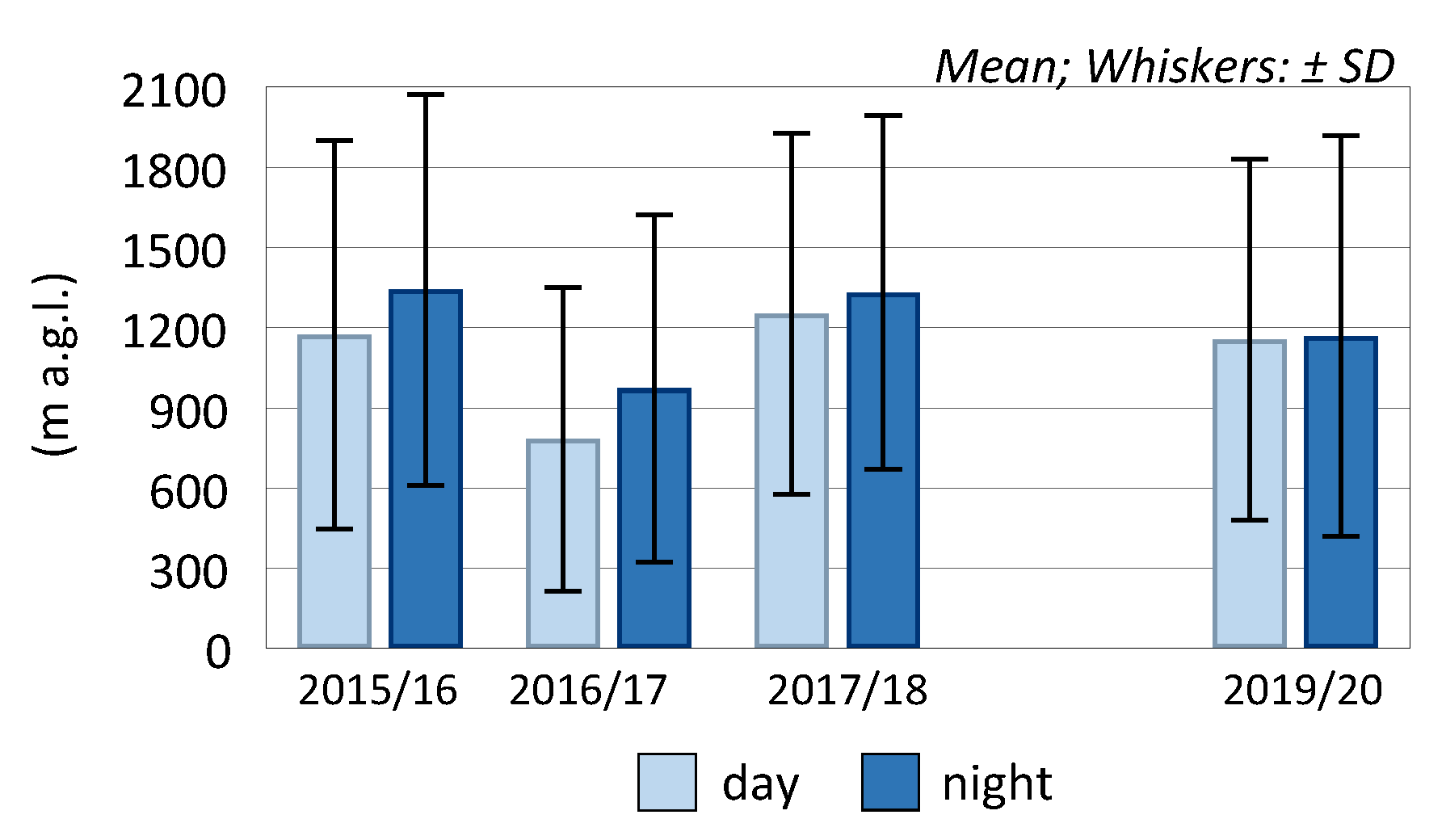
3.1.2. Thickness and Strength

Thickness of SBI layers is a particularly important feature with respect to cities where low emissions are predominant. The increase in the thickness, as well as in the inversion temperature gradient, hinders the movement and air exchange which directly results in an increase in the concentration of pollutants. In three winter seasons, from December 2015 to February 2018, significantly greater thickness was recorded in the case of SBI occurring at night-time, with particularly great thickness (approx. 430 m) recorded in the winter of 2016/17 (Figure 3). The thickness of daytime SBI in these seasons did not exceed 200 m. The last winter season proved to be atypical, as the SBI showed comparable thickness during night-time and daytime.
The mean intensity of daytime and night-time SBI ranged from approx. 0.2 to 1.2 °C; however, greater variability between winters was found for daytime inversions. In the winter of 2016/17, the intensity of daytime inversions was the greatest (around 1 °C) and slightly exceeded the intensity of night-time inversions. However, in the remaining winter seasons, night-time inversions showed greater intensity. The maximum values of the inversion gradient did not exceed 4 °C.
The thickness of ELI, forming at the altitude of approx. 3000 m a.g.l, was found to have a greater variability in comparison with SBI—the exception was the night-time of the winter season 2016/17. The discussed feature of ELI showed lower variability between the winter seasons in both times of the 24 h period. The thickest ELIs (approx. 250 m) were identified in the winter of 2016/17, while in the remaining seasons the thickness ranged from 160 to 230 m. Elevated inversions were characterised not only by a markedly greater intensity as compared with surface-based inversions but also by an incomparably greater range of variation. In all winter seasons, both during daytime as well as night-time, the mean intensity exceeded 1.2 °C and the average elevated inversions with the highest intensity (1.8 °C) occurred during daytime in the winter of 2017/18. The most intense ELIs (inversion gradient approx. 12 °C) were recorded during night-time in the winter season 2015/16, and during daytime in the winter of 2017/18.

3.1.3. Base of the ELI

The location of the base of the elevated, yet the lowest, inhibition layer can be considered as the altitude of the turbulent mixing of pollutants. As is presented in Figure 4, the ELIs with the lowest locations, limiting the altitude of such a mixing layer, generally formed at the altitude of approx. 1200 m. The inversions with the lowest location, in both times of the 24 h period, were determined for the winter of 2016/17, which was characterised by, on average, the highest PM concentrations (Figure 5). During this winter season, daytime inversions formed at an altitude of approx. 800 m.

3.2. Particulate Matter Concentrations

From the four analysed winter seasons (December–February), by far the highest concentration of both PM fractions was recorded in the first two seasons, i.e., 2015/16 and 2016/17 (Figure 5). PM10 concentrations recorded in the aforementioned winter seasons, both during the daytime (07:00–18:00) as well as night-time (19:00–06:00), exceeded 50 µg·m−3, whereas in the winter of 2017/18 and particularly in the winter of 2019/20, the recorded PM10 concentration was approx. two times lower. By far the lowest PM concentration in the winter season of 2019/20 resulted from atypical thermal conditions occurring in all months. The results of the analyses given in the Bulletin of Monitoring Climate in Poland [33] indicate that December 2019 and February 2020 were extremely warm, and January was anomalously warm. The mean monthly air temperatures in three months of the season recorded in Wrocław were from 4 to 5 °C higher than the norm. The winters of 2016/17 and 2017/18 were classified as normal. The winter of 2015/16 was classified as anomalously warm, yet this was due to extremely warm December and anomalously warm February, whereas January was slightly cold. Nevertheless, the fact that mean seasonal particulate matter concentration recorded in the anomalously warm winter of 2015/16 was by far higher than that recorded in 2019/20 only confirms the role of other factors determining the volume and variability of pollutants concentration, and not only the role of emissions—in the case of Poland, PM mainly from the thermal energy production sector.
In all analysed winters, the found air pollution with particulate matter was mainly determined by the fraction with an aerodynamic diameter of 2.5 µm, considered by the WHO to be the most harmful to health. As transpires from the analysis of data presented in Figure 5, in the winter seasons of 2016/17, 2017/18 and 2019/20, PM2.5 concentrations were only 3 to 8 μg·m−3 lower than that of PM10. A markedly lower share of particulate matter fraction of <2.5 µm in the particulate matter pollution was found in the first of the analysed winter seasons—daytime and night-time PM2.5 concentrations were lower than that of PM10 by 18 and 13 μg·m−3, respectively.
The very high share of particulate matter fraction < 2.5 μg in pollution with particulate matter is evidenced by the results from a series of previous winter seasons (2009/10–2014/15) recorded all over the country. In some regions of Poland, the hourly particulate matter concentrations, which generally fell between 0 and 75 μg·m−3, were recorded more frequently with respect to PM2.5 than PM10, in a longer, i.e., 10 year-long, series of winter seasons (2005/06–2014/15) [34].
Higher concentrations of particulate matter were recorded during the night-time; however, in the case of PM10, the differences between the mean night-time and daytime concentrations were minor and only slightly greater in the case of PM2.5.

3.3. Cluster Analysis
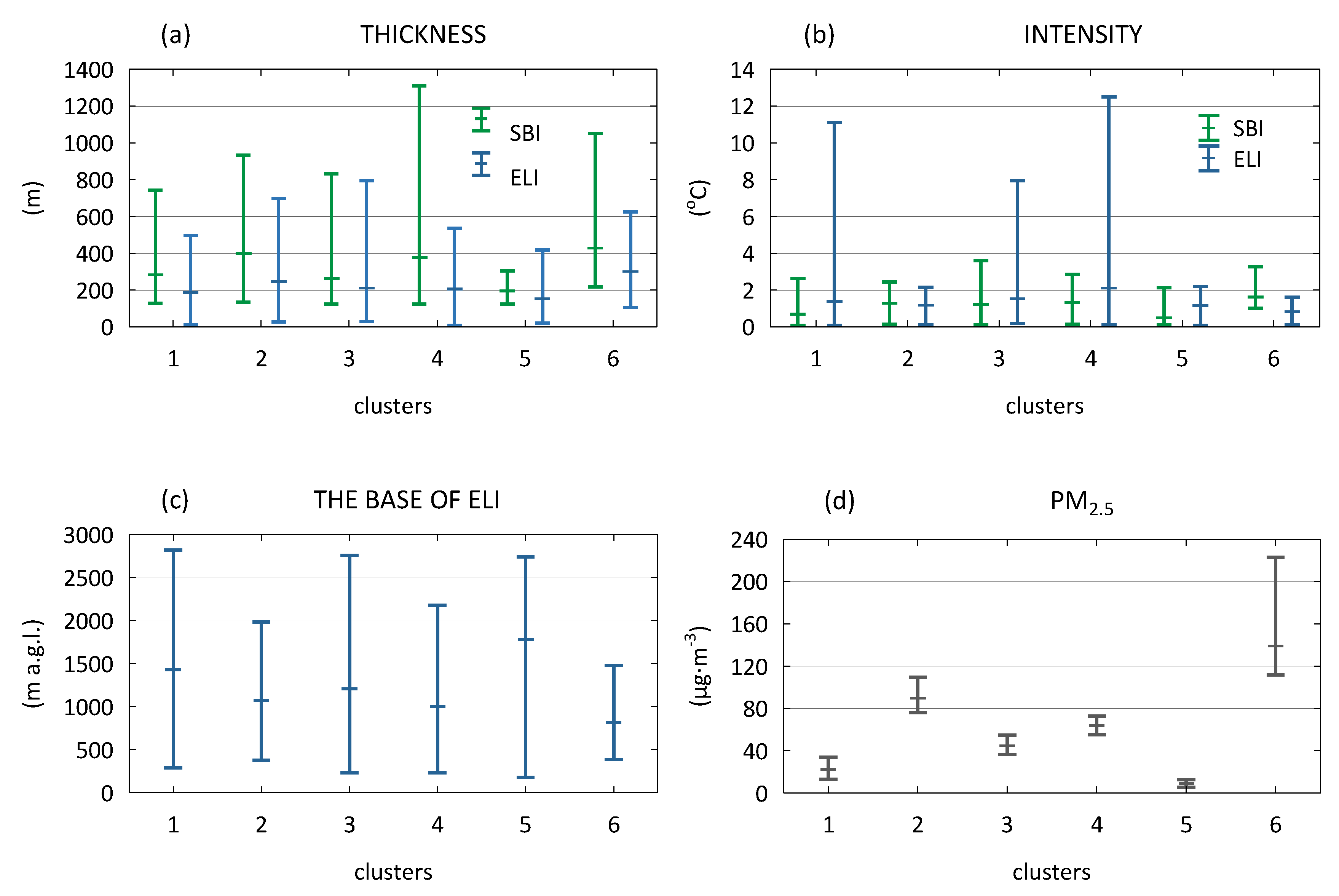
The relationship between PM concentration with the occurrence of TI, proved in numerous studies [11,13,14,15,16,35,36,37], is indicated by the assessment of the variability of PM10 and PM2.5 concentrations against the thickness of both types of inversion layers in each of the analysed winter seasons, and also in the contrastive winter seasons with respect to concentrations, i.e., 2016/17 and 2019/20 (Figure 6). In many cases, the rapid increase in the concentrations of both PM fractions were recorded during the day or night, characterised by a greater thickness of SBI and elevated layers of lower location and greater thickness. In both winter seasons, the negative role of SBI occurring in sequences of consecutive nights was pronounced.
The assessment of the influence of inversion layers on the concentration of particulate matter with the use of the cluster analysis was conducted in different versions: both the qualitative classification of PM10 and PM2.5 concentrations as well as the effect of inversion layers separately per type and times of the 24 h period. The main difficulty while assessing the final results was related to a clearly lower frequency of SBI, particularly in the daytime. The results of the cluster analysis, taking into consideration both inversion types and without the division into times of the 24 h period, separately for PM10 and PM2.5, were adopted as final. This is supported by the fact that the concentration values is determined by both types of inversion [11,12], and their effects are not limited merely to the time of occurrence. The results in line with this approach are presented in Tables 1 and 2 and Figures 7 and 8.

3.3.1. TI and PM10

In the four analysed winter seasons, PM10 concentrations in the conditions of temperature inversion were classified into six clusters representative of five air quality classes (Table 1 and Figure 7). Mean daytime and mean night-time PM10 concentrations showed wide fluctuations—from approx. 16 µg·m−3 in cluster 4, representative of very good air quality, to 140 µg·m−3 in cluster 2, which mainly includes cases of bad air quality, with four cases of very bad air quality. Cluster 2, encompassing cases of the worst air quality, was marked by the greatest range of mean concentrations—from approx. 110 to 240 µg·m−3. As for the remaining clusters, the differences between max and min concentrations did not exceed 30 µg·m−3 (Figure 7). The worst air quality due to PM10 concentration was recorded around two times less frequently than very good air quality.
The characteristics of the analysed features of inversion layers in particular clusters indicate that some of the features at times generated diverse and, at other times, contrastive air quality. Bad and very bad air quality was mostly determined by significantly the greatest, over 300 m, thickness of ELI. Such situations were accompanied by a greater thickness and intensity of SBI, yet with comparable characteristics of SBI, the concentrations of PM10 were classified into cluster 6—representative of good air quality. Very good air quality (cluster 4) was predominantly determined by the lowest thickness of both types of inversion, i.e., SBI and ELI, which at the same time showed the smallest spread, particularly in the case of surface-based layers (Figure 7).
Surprisingly, two separate clusters (1 and 6) were marked—each cluster encompassed comparable PM10 concentrations, classified as a good air quality state. In order to provide an explanation for this phenomenon, the cases of concentrations classified to particular air quality classes per winter seasons, taking into consideration the months and times of the 24 h period, i.e., day and night, were compared. The analysis conducted in the aforementioned way revealed interesting findings. PM10 concentrations indicating good air quality, classified as cluster 1 and 6, were found in all analysed winter seasons; however, unlike other clusters, they were mostly limited to night-time concentrations. In cluster 6, there were only 3 cases of daytime concentrations.
In cluster 1, good air quality was identified at a slightly lower (by approx. 37 m) thickness, yet at twice the intensity of SBI, but most of all at a significantly higher thickness (as much as by 75 m) of ELI occurring at a lower altitude by almost 2.5 times in comparison to cluster 6. The contrastive characteristics between the two clusters were also found with respect to the variability of thickness and the altitude of the base of ELI—very high for cluster 1 and very low for cluster 6 (Figure 7).
Verification and explanation for the occurrence of this phenomenon requires analysis based on a longer measurement series, especially given the much less frequent occurrence of SBI. Moreover, keeping in mind that pollutant concentrations result from emissions and meteorological conditions determining their dispersion, apart from inversions, the analysis should include the most important elements, the role of which was indicated in numerous studies [14,38,39]. However, at this particular stage of the study, an explanation for this issue may be provided by the fact that, depending on the feature of inversion, the analysed relationships showed differences in terms of slope. The concentration of pollutants manifested an increase in the conditions of great thickness of both inversion types, whereas the unequivocally positive feature was the high location of the base of elevated inversion. This was proven not only with respect to PM but also other types of pollutants, both by long series as well as individual winter seasons, and even particular months and times in the 24 h period [12,29].

3.3.2. TI and PM2.5

Classification of PM2.5 concentrations, depending on the occurrence of temperature inversions, produced six clusters; however, unlike in the case of PM10, each cluster represented another air quality class, with the very bad class in an individual cluster. Moreover, all considered features of inversions clearly demonstrated conditions in which air quality was very bad (cluster 6) and very good (cluster 5) (Table 2). Very bad air quality (the mean of daytime and night-time), around 140 µg·m−3, was identified at the greatest thickness of SBI and ELI, respectively—approx. 430 and 300 m—and ELI occurred at a significantly lower altitude i.e., around 820 m. Additionally, SBI was characterised by a high intensity at −1.6 °C. The contrastive features of inversion layers were represented by conditions in which air quality was very good (mean concentration approx. 9 µg·m−3). Above all else, these conditions are: twice as low thickness of SBI, showing little intensity (approx. 200 m), but also of ELI (around 150 m), which occurred at almost twice the altitude—approx. 1800 m. In the four analysed winter seasons, the extreme air quality levels were identified rarely—very bad in around 6% of days and nights, and very good in around 7%. Concentrations of PM2.5 classified as very bad air quality were characterised by a large range of variability—from 110 to 230 µg·m−3 (Figure 8d).
Almost half of the days and nights (approx. 45%) were characterised by good air quality (cluster 1). In comparison with the clusters encompassing bad, moderate and sufficient air quality classes, the inversion conditions of good air quality were mostly characterised by more favourable features of elevated inversions, higher location of the base and lower thickness, with rather high variation in intensity (Figure 8b). Deterioration of air quality from moderate, through sufficient to bad in clusters 3, 4 and 2 respectively, is characterised by a great conformity with increasing thickness of SBI of comparable intensity. In the case of sufficient and bad air quality (clusters 4 and 2), the relationships between the concentrations and characteristics of ELI are not as unequivocal. For example, sufficient air quality (cluster 4) occurred on days and nights when the most intense (around 2 °C) ELI formed approx. 70 m lower, yet showed lower thickness than in the conditions accompanying bad air quality (cluster 2). Bad air quality was identified as occurring as a result of, among others, layers of higher location yet of significantly greater thickness and much smaller intensity. This is yet another example of how features of opposite impacts (a positive role of high location of the base and the negative role of high thickness) may compensate for one another in terms of air quality.

4. Conclusions

The results presented in the study show the usefulness of cluster analysis in the assessment of the role of the types and dominant features of temperature inversion in determining the concentration of particulate matter. Even though the analysis covers only four winter seasons, the applied method conclusively manifested the features of surface-based and elevated inversions in which air quality is classified into contrastive classes, i.e., very bad and very good—this is found with respect to both analysed PM fractions. A drastic decrease in air quality, from very good to very bad, due to both PM10 and PM2.5 concentrations, was reported in the conditions of approx. twice the thickness of SBI and ELI of the lowest location, the base of which formed at less than half the altitude. Furthermore, such contrastive deterioration of air quality occurred at almost three times greater intensity surface based inversions; however, it is difficult to assess the role of this feature with respect to elevated inversion.

Author Contributions

Conceptualization, J.N.-L.; methodology, J.N.-L. and M.C.; software, J.N.-L.; formal analysis, J.N.-L. and M.C.; data curation, J.N.-L. and M.C.; writing—original draft preparation, J.N.-L. and M.C.; writing—review and editing, J.N.-L. and M.C.; visualization, J.N.-L. and M.C. Both authors have read and agreed to the published version of the manuscript.

Funding

This research received no external funding.

Conflicts of Interest

The authors declare no conflict of interest.

References

  1. Stryhal, J.; Huth, R.; Sládek, I. Climatology of low-level temperature inversions at the Prague-Libuš aerological station. Appl. Clim. 2015, 127, 409–420. [Google Scholar] [CrossRef]
  2. Czarnecka, M.; Nidzgorska-Lencewicz, J.; Rawicki, K. Temporal structure of thermal inversions in Łeba (Poland). Appl. Clim. 2018, 136, 13. [Google Scholar] [CrossRef] [Green Version]
  3. Palarz, A.; Celiński-Mysław, D.; Ustrnul, Z. Temporal and spatial variability of surface-based inversions over Europe based on ERA-Interim reanalysis. Int. J. Clim. 2018, 38, 158–168. [Google Scholar] [CrossRef]
  4. Palarz, A.; Celiński-Mysław, D.; Ustrnul, Z. Temporal and spatial variability of elevated inversions over Europe based on ERA-Interim reanalysis. Int. J. Clim. 2020, 40, 1335–1347. [Google Scholar] [CrossRef]
  5. Devasthale, A.; Willén, U.; Karlsson, K.-G.; Jones, C.G. Quantifying the clear-sky temperature inversion frequency and strength over the Arctic Ocean during summer and winter seasons from AIRS profiles. Atmos. Chem. Phys. Discuss. 2010, 10, 5565–5572. [Google Scholar] [CrossRef] [Green Version]
  6. Zhang, Y.; Seidel, D.J.; Golaz, J.-C.; Deser, C.; Tomas, R.A. Climatological Characteristics of Arctic and Antarctic Surface-Based Inversions. J. Clim. 2011, 24, 5167–5186. [Google Scholar] [CrossRef] [Green Version]
  7. Knozová, G. Temperature inversions at Prague-Libuš aerological stadion (1975–2006). In Klimat i Bioklimat Miast; Kłysik, K., Wibig, J., Fortuniak, K., Eds.; Wydawnictwo Uniwersytetu Łódzkiego, Katedra Meteorologii i Klimatologii UŁ: Łódź, Poland, 2008; pp. 65–80. (In Polish) [Google Scholar]
  8. Brümmer, B.; Schultze, M. Analysis of a 7-year low-level temperature inversion data set measured at the 280 m high Hamburg weather mast. Meteorol. Z. 2015, 24, 481–494. [Google Scholar] [CrossRef]
  9. Joly, D.; Richard, Y. Frequency, intensity, and duration of thermal inversions in the Jura Mountains of France. Appl. Clim. 2019, 138, 639–655. [Google Scholar] [CrossRef]
  10. Bourne, S.; Bhatt, U.; Zhang, J.; Thoman, R. Surface-based temperature inversions in Alaska from a climate perspective. Atmos. Res. 2010, 95, 353–366. [Google Scholar] [CrossRef]
  11. Czarnecka, M.; Nidzgorska-Lencewicz, J. The impact of thermal inversion on the variability of PM10 concentration in winter seasons in Tricity. Environ. Prot. Eng. 2017, 43, 157–172. [Google Scholar] [CrossRef]
  12. Nidzgorska-Lencewicz, J.; Czarnecka, M.; Rawicki, K. Thermal inversions and sulphure dioxide concentrations in some Polish cities in the winter season. J. Elem. 2016, 21, 1001–1015. [Google Scholar] [CrossRef]
  13. Malek, E.; Davis, T.; Martin, R.S.; Silva, P.J. Meteorological and environmental aspects of one of the worst national air pollution episodes (January, 2004) in Logan, Cache Valley, Utah, USA. Atmos. Res. 2006, 79, 108–122. [Google Scholar] [CrossRef]
  14. Nidzgorska-Lencewicz, J.; Czarnecka, M. Winter Weather Conditions vs. air quality in Tricity, Poland. Appl. Clim. 2014, 119, 611–627. [Google Scholar] [CrossRef] [Green Version]
  15. Largeron, Y.; Staquet, C. Persistent inversion dynamics and wintertime PM10 air pollution in Alpine valleys. Atmos. Environ. 2016, 135, 92–108. [Google Scholar] [CrossRef]
  16. Hu, Y.; Wang, S.; Ning, G.; Zhang, Y.; Wang, J.; Shang, Z. A quantitative assessment of the air pollution purification effect of a super strong cold-air outbreak in January 2016 in China. Air Qual. Atmos. Health 2018, 11, 907–923. [Google Scholar] [CrossRef]
  17. Rogula-Kozłowska, W.; Klejnowski, K.; Rogula-Kopiec, P.; Ośródka, L.; Krajny, E.; Błaszczak, B.; Mathews, B. Spatial and seasonal variability of the mass concentration and chemical composition of PM2.5 in Poland. Air Qual. Atmos. Health 2014, 7, 41–58. [Google Scholar] [CrossRef] [PubMed] [Green Version]
  18. Majewski, G.; Rogula-Kozłowska, W.; Rozbicka, K.; Rogula-Kopiec, P.; Mathews, B.; Brandyk, A. Concentration, Chemical Composition and Origin of PM1: Results from the First Long-term Measurement Campaign in Warsaw (Poland). Aerosol Air Qual. Res. 2018, 18, 636–654. [Google Scholar] [CrossRef]
  19. Sówka, I.; Chlebowska-Styś, A.; Pachurka, Ł.; Rogula-Kozłowska, W.; Mathews, B.; Styś, C.; Kozłowska, R. Analysis of Particulate Matter Concentration Variability and Origin in Selected Urban Areas in Poland. Sustainability 2019, 11, 5735. [Google Scholar] [CrossRef] [Green Version]
  20. Medina, S. Apheis: Public health impact of PM10 in 19 European cities. J. Epidemiol. Community Health 2004, 58, 831–836. [Google Scholar] [CrossRef] [Green Version]
  21. Shi, L.; Zanobetti, A.; Kloog, I.; Coull, B.A.; Koutrakis, P.; Melly, S.J.; Schwartz, J.D. Low-Concentration PM 2.5 and Mortality: Estimating Acute and Chronic Effects in a Population-Based Study. Environ. Health Perspect. 2016, 124, 46–52. [Google Scholar] [CrossRef] [Green Version]
  22. Widziewicz, K.; Rogula-Kozlowska, W.; Loska, K.; Kociszewska, K.; Majewski, G. Health Risk Impacts of Exposure to Airborne Metals and Benzo(a)Pyrene during Episodes of High PM10 Concentrations in Poland. Biomed. Environ. Sci. 2018, 31, 23–36. [Google Scholar] [PubMed]
  23. Zwozdziak, A.; Gini, M.I.; Samek, L.; Rogula-Kozlowska, W.; Sowka, I.; Eleftheriadis, K. Implications of the aerosol size distribution modal structure of trace and major elements on human exposure, inhaled dose and relevance to the PM2.5 and PM10 metrics in a European pollution hotspot urban area. J. Aerosol Sci. 2017, 103, 38–52. [Google Scholar] [CrossRef]
  24. OECD. Environmental Outlook to 2050, the Consequences of Inaction; Organisation for Economic Co-Operation and Development Publishing: Paris, France, 2012. [Google Scholar]
  25. European Environment Agency. EMEP/EEA Air Pollutant Emission Inventory Guidebook 2019; Technical Guidance to Prepare National Emission Inventories, EEA Report No 13/2019; European Environment Agency: Copenhagen K, Denmark, 2019.
  26. Available online: http://weather.uwyo.edu/upperair/sounding.html (accessed on 10 December 2020).
  27. Parczewski, W. Thermal Blocking Layers in Poland; Prace Instytutu Meteorologii i Gospodarki Wodnej: Warszawa, Poland, 1976; p. 8. (In Polish) [Google Scholar]
  28. Chief Inspectorate Of Environmental Protection. Available online: www.gios.gov.pl (accessed on 10 December 2020).
  29. Ocena Jakości Powietrza—Bieżące dane Pomiarowe—GIOŚ. Available online: http://powietrze.gios.gov.pl/pjp/current (accessed on 10 December 2020).
  30. Govender, P.; Sivakumar, V. Application of k-means and hierarchical clustering techniques for analysis of air pollution: A review (1980–2019). Atmos. Pollut. Res. 2020, 11, 40–56. [Google Scholar] [CrossRef]
  31. Walczewski, J. Some data on occurrence of the all-day inversions in the atmospheric boundary-layer in Cracow and on the factors stimulating this occurrence. Przegląd Geofizyczny 2009, 54, 183–191. (In Polish) [Google Scholar]
  32. Czarnecka, M.; Nidzgorska-Lencewicz, J.; Rawicki, K. Thermal conditions and air pollution in selected Polish cities during the winter period 2016/2017. Sci. Rev. 2017, 26, 437–446. (In Polish) [Google Scholar] [CrossRef] [Green Version]
  33. Biuletyn Monitoringu Klimatu Polski—Portal Klimat IMGW-PiB. Available online: https://klimat.imgw.pl/pl/biuletyn-monitoring/ (accessed on 10 December 2020).
  34. Rawicki, K.; Czarnecka, M.; Nidzgorska-Lencewicz, J. Regions of pollution with particulate matter in Poland. In Proceedings of the E3S Web of Conferences, Polanica-Zdrój, Poland, 16–20 April 2018; Volume 28, p. 1025. [Google Scholar]
  35. Palarz, A.; Celiński-Mysław, D. The effect of temperature inversions on the particulate matter PM10 and sulfur dioxide concentrations in selected basins in the Polish Carpathians. Carpathian J. Earth Environ. Sci. 2017, 12, 629–640. [Google Scholar]
  36. Xu, T.; Song, Y.; Liu, M.; Cai, X.; Zhang, H.; Guo, J.; Zhu, T. Temperature inversions in severe polluted days derived from radiosonde data in North China from 2011 to 2016. Sci. Total. Environ. 2019, 647, 1011–1020. [Google Scholar] [CrossRef]
  37. Sabatier, T.; Paci, A.; Canut, G.; Largeron, Y.; Dabas, A.; Donier, J.-M.; Douffet, T. Wintertime Local Wind Dynamics from Scanning Doppler Lidar and Air Quality in the Arve River Valley. Atmosphere 2018, 9, 118. [Google Scholar] [CrossRef] [Green Version]
  38. Zuśka, Z.; Kopcińska, J.; Dacewicz, E.; Skowera, B.; Wojkowski, J.; Ziernicka-Wojtaszek, A. Application of the Principal Component Analysis (PCA) Method to Assess the Impact of Meteorological Elements on Concentrations of Particulate Matter (PM10): A Case Study of the Mountain Valley (the Sącz Basin, Poland). Sustainability 2019, 11, 6740. [Google Scholar] [CrossRef] [Green Version]
  39. Żyromski, A.; Biniak-Pieróg, M.; Burszta-Adamiak, E.; Zamiar, Z. Evaluation of Relationship Between Air Pollutant Concentration and Meteorological Elements in Winter Months. J. Water Land Dev. 2014, 22, 25–32. [Google Scholar] [CrossRef] [Green Version]
Figure 1. Location of the measuring stations in Wrocław (Poland).
Atmosphere 11 01351 g001
Figure 2. Frequency (%) of the surface-based (SBI) and elevated (ELI) inversion layers.
Atmosphere 11 01351 g002
Figure 3. Thickness and strength of the SBI (a,b) and ELI (c,d) inversion layers. SD—standard deviation.
Atmosphere 11 01351 g003
Figure 4. The base of the first (located at the lowest level) ELI layers.
Atmosphere 11 01351 g004
Figure 5. Average concentrations (μg·m–3) of PM10 and PM2.5 during calendar winter (December–February).
Atmosphere 11 01351 g005
Figure 6. Distribution of the night-time and daytime concentration of PM10 and PM2.5 in Wrocław in relation to the course of TI; winter 2016/17 and 2019/20.
Atmosphere 11 01351 g006
Figure 7. Basic characteristics (mean and min-max) of TI layers (ac) and PM10 (d) in selected clusters. Air quality in distinct clusters: 1—good, 2—very bad and bad, 3—moderate, 4—very good, 5—sufficient, 6—good.
Atmosphere 11 01351 g007
Figure 8. Basic characteristics (mean and min-max) of TI layers (ac) and PM2.5 (d) in selected clusters. Air quality in distinct clusters: 1—good, 2—bad, 3—moderate, 4—sufficient, 5—very good, 6—very bad.
Atmosphere 11 01351 g008
Table 1. Characteristics of inversion layers and PM10 concentrations in distinct clusters.
ClustersCharacteristics of Inversion LayersPM10
(µg·m−3)
Number of CasesPercentage
(%)
SBIELI
Thickness
(m)
Intensity
(°C per 100 m)
Base
(m a.g.l.)
Thickness
(m)
Intensity
(°C)
1 a280.21.2769.1255.01.335.42619.0
  b±51.3±0.4±163.9±65.0±0.4±3.2
2 a400.31.4764.1307.71.0136.0128.8
  b±145.7±0.5±216.3±123.9±0.3±22.4
3 a305.81.11118.8184.21.364.33324.1
  b±79.8±0.2±212.3±56.6±0.5±3.0
4 a205.90.51702.9148.01.215.52115.3
  b±28.9±0.2±336.8±49.4±0.4±1.9
5 a421.11.41172.3225.61.891.81410.2
  b±153.5±0.5±310.8±112.0±1.3±4.3
6 a316.70.61879.0180.31.632.33122.6
  b±62.4±0.2±181.4±46.1±0.8±2.7
a—mean; b—confidence level at 95%; air quality in distinct clusters: 1—good, 2—very bad and bad, 3—moderate, 4—very good, 5—sufficient, 6—good.
Table 2. Characteristics of inversion layers and PM2.5 concentrations in distinct clusters.
ClustersCharacteristics of Inversion LayersPM2.5
[µg·m−3]
Number of CasesPercentage
[%]
SBIELI
Thickness
(m)
Intensity
(°C per 100 m)
Base
(m a.g.l.)
Thickness
(m)
Intensity
(°C)
1 a284.70.71428.5188.01.422.66944.5
  b±31.0±0.1±170.4±25.9±0.4±1.5
2 a398.61.31076.4247.21.289.7159.7
  b±135.2±0.4±309.7±120.7±0.3±6.2
3 a261.71.21209.2211.21.545.03120.0
  b±45.9±0.3±232.5±70.3±0.5±2.1
4 a378.21.31004.1204.92.163.82012.9
  b±132.4±0.4±254.4±69.5±1.5±2.7
5 a194.20.51780.1153.61.29.3117.1
  b±38.3±0.4±509.8±91.9±0.5±1.7
6 a429.71.6817.9300.40.8139.095.8
  b±200.8±0.6±289.1±125.0±0.4±27.0
a—mean; b—confidence level at 95%; air quality in distinct clusters: 1—good, 2—bad, 3—moderate, 4—sufficient, 5—very good, 6—very bad.
Publisher’s Note: MDPI stays neutral with regard to jurisdictional claims in published maps and institutional affiliations.

