Impact of Urban Canopy Parameters on a Megacity’s Modelled Thermal Environment

Abstract

Urban canopy parameters (UCPs) are essential in order to accurately model the complex interplay between urban areas and their environment. This study compares three different approaches to define the UCPs for Moscow (Russia), using the COSMO numerical weather prediction and climate model coupled to TERRA_URB urban parameterization. In addition to the default urban description based on the global datasets and hard-coded constants (1), we present a protocol to define the required UCPs based on Local Climate Zones (LCZs) (2) and further compare it with a reference UCP dataset, assembled from OpenStreetMap data, recent global land cover data and other satellite imagery (3). The test simulations are conducted for contrasting summer and winter conditions and are evaluated against a dense network of in-situ observations. For the summer period, advanced approaches (2) and (3) show almost similar performance and provide noticeable improvements with respect to default urban description (1). Additional improvements are obtained when using spatially varying urban thermal parameters instead of the hard-coded constants. The LCZ-based approach worsens model performance for winter however, due to the underestimation of the anthropogenic heat flux (AHF). These results confirm the potential of LCZs in providing internationally consistent urban data for weather and climate modelling applications, as well as supplementing more comprehensive approaches. Yet our results also underline the continued need to improve the description of built-up and impervious areas and the AHF in urban parameterizations.

1. Introduction

For long, urban-induced meteorological effects such as the well-known urban heat island (UHI) [1] have been a primary focus in the urban climate research community. Yet recently, the role of cities in climate adaptation and mitigation practices is acknowledged to be a core part of global initiatives, with a need for reliable climate and meteorological observations, modelling capabilities and associated services to support disaster risk management, urban planning and governance [2,3,4,5]. High-resolution city-scale atmospheric models are an essential tool for such services, needed for example, for numerical weather prediction (NWP) applications [6,7], regional-scale heat stress assessments, and the development of sustainable urban areas safeguarding livability in cities [8,9].

Despite recent advances in building-resolving urban atmospheric models [10,11], it is still not possible to integrate such fine-scale approaches into an operational NWP or long-term regional and global climate models. Therefore, so-called urban canopy models (UCMs) are used to parameterize the interactions between the urbanised surface and the atmosphere above in meso-scale atmospheric models [12]. Regardless the degree of complexity, the UCMs assume that the model grid cell or its parts are occupied by a homogeneous urban environment, whose characteristics are described by a number of urban canopy parameters (UCPs). The success of meteorological modelling for urbanised regions is largely determined by the accuracy of specifying these UCPs.

Acquiring detailed UCP data for urban areas is not trivial. Many studies deal with the problem of UCP quantification [13], but the choice of the optimal method is still debatable. The most comprehensive UCP datasets are sourced from 2.5 or 3D vector building datasets, provided by official authorities [14,15,16] or derived from crowd-sourced cartographic services such as OpenStreetMap [17]. Such detailed building datasets are considered as the best available source to retrieve UCPs related to urban morphology, while the land cover and vegetation properties could be effectively derived from high-resolution satellite images [18]. Therefore, the most advanced approaches of UCP definition are based on the combined use of the vector spatial data and satellite images [19]. However, such comprehensive approaches developed for different cities lack uniformity. Their application for new areas is strongly limited by the presence and quality of the vector datasets, which are often not available, have restricted access or are outdated for fast-developing cities in emerging countries [20,21,22]. Additionally, the procedure of UCP calculation from the detailed vector data requires computationally-demanding processing in Geographic Information Systems (GIS), which cannot always be fully automated. Therefore, the limited access to official data, the absence of uniform standards for its structure, the variable quality of the crowdsourcing information, and high demands in labour and computation resources limit the application of comprehensive GIS-based approaches on a scale bigger than one city or one region.

The concept of the Local Climate Zones (LCZs) suggested by Stewart and Oke (2012) [23] is considered to be a universal classification for urban climate studies that not only provides a common platform for knowledge exchange and a pathway to model applications in cities with little data infrastructure, but also quantifies UCPs that are key in urban ecosystem processes [1,23,24,25,26]. For specific urban areas, comprehensive information about the three-dimensional urban morphology and material properties might be available. Yet generally, we know very little worldwide on city form and functions or the UCPs, being a major obstacle for state-of-the-art science models [13,27]. WUDAPT, the World Urban Database and Access Portal Tool project (www.wudapt.org) [27], addresses this issue by “striving to provide urban canopy information and modelling infrastructure to facilitate urban-focused climate, weather, air quality, and energy-use modelling application studies”. Baseline parameter ranges are provided by Stewart and Oke [23] for sky view factor, aspect ratio, building surface fraction, impervious and pervious surface fractions, height of roughness elements, surface admittance, surface albedo, anthropogenic heat flux (see their Tables 3 and 4). On the one hand, these default ranges have been shown to match well with high-resolution independent auxiliary datasets as shown by Demuzere et al. [26,28] over continental Europe and the continental United States. On the other hand, others have shown that the default ranges provided by Stewart and Oke [23], in an urban canopy model context, overall provide similar modelling results compared to using GIS-based datasets [29,30,31]. Not surprisingly, these studies all use the Weather and Research Forecasting (WRF) model [32], in part because of the availability of the “WUDAPT to WRF” (W2W) tool, an outcome of the work by Brousse et al. [33], and recently fine-tuned by Zonato et al. [34]. The tool adjusts WRF’s default urban classes to the ten urban Local Climate Zones, and simultaneously provides LCZ specific UCPs.

This study extends the philosophy of LCZ-derived UCPs to the COSMO limited-area atmospheric model and its climate version COSMO-CLM [35] coupled to the TERRA_URB urban parameterization developed by Wouters et al. [36]. We present an open-source tool “WUDAPT to COSMO” (W2C) that translates and regrids LCZ maps to UCPs required for TERRA_URB, which is evaluated using a series of numerical experiments over the megacity of Moscow (Russia). In order to evaluate the advantages and shortcomings of the LCZ-based approach, we present its comparison with the default UCP input for TERRA_URB from global databases and with a reference UCP dataset, derived by a comprehensive GIS-based approach using OpenSteetMap vector data, Sentinel-2 satellite images and a Copernicus Global Land Cover raster dataset.

2. Materials and Methods

2.1. Study Area

Moscow is the biggest Russian megacity with population of approximately 17 million people [37]. The area of the city as an administrative unit encompasses 2561 km${}^2$, which, since 2011, includes a large area known as “New Moscow”, that to date remains practically undeveloped. The actual area of the city (excluding the suburbs and satellite cities) covers approximately 1000 km${}^2$. The city is densely built with predominantly mid- and high-rise block-houses, has a compact and relatively symmetric shape and is surrounded by a flat and homogeneous terrain, covered mostly by forests or croplands [38,39].

Moscow has a temperate continental climate (Dfb in the Köppen climate classification) with a mean annual temperature of $5.8$ ${}^{\circ }$C and mean June and January temperatures of $19.2$ ${}^{\circ }$C and $-6.5$ ${}^{\circ }$C respectively. Due to its cold winters Moscow is known as one of the world’s coldest megacities. The intense urban-induced meteorological effects of Moscow are easy to detect against the homogeneous rural and suburban surroundings, which turns the city to a convenient site for urban climate research. The city has experienced an increasing UHI intensity trend over the last decades [40], with a present-day annual-mean UHI intensity of 2${}^{\circ }$ peaking to more than 10 ${}^{\circ }$C during calm and clear nights [41,42]. Its relevance as a test-bed for model testing and verification is shown by previous studies using COSMO model with the TERRA_URB scheme [6,39,43].

2.2. The COSMO Model and TERRA_URB Scheme

COSMO is a limited-area non-hydrostatic model developed by the COSMO consortium (Consortium for Small-scale Modelling, [44]). The model is used for numerical weather prediction in many countries including Russia [6]. The model version COSMO-CLM or CCLM [35], developed by the CLM (Climate Limited-area Modeling) community) [45], is adopted for long-term simulations and is widely used in regional climate studies.

The bulk urban canopy parameterization TERRA_URB in COSMO uses the Semi-empirical URban canopy dependencY algorithm (SURY [36]) to condense the three dimensional urban canopy information to a limited number of bulk properties, thereby strongly reducing the computational cost without loss of performance [36,46,47]. TERRA_URB was originally implemented in the COSMO-CLM version $5.0\_clm9$ as a separate branch of the model development. This version was successfully used for urban climate simulations in global cities [20,21,24,39,43,46,47,48,49]. Recently, the TERRA_URB scheme was implemented to a newer version of COSMO ($5.05urb$, used in the current study) as part of the AEVUS (Analysis and evaluation of the TERRA_URB scheme) priority task of the COSMO consortium [6,50]. This newer version includes improved boundary-layer physics and is unified with the recent developments of the ICON (ICOsahedral Nonhydrostatic) modelling system [51,52]. In the near future, TERRA_URB is planned to be implemented to the major branch of COSMO (version $6.0$) and ICON.

The urban environment in TERRA_URB is described by the following UCPs. The impervious area fraction (ISA) is the most critical parameter, as it defines urban tile, that is, the part of a model grid cell where the TERRA_URB scheme is applied within the framework of a so-called poor-man’s tile approach [36]. This part of a model grid cell is assumed to be completely paved and devoid of vegetation. For this fraction of the grid cell, the semi-empirical corrections are applied for the land surface parameters in order to take into account the geometric, radiative and thermal properties of the built environment considering the morphological UCPs (building plan area fraction in urban tile, R (called as roof fraction in Reference [36]); mean building height, H; mean aspect ratio of the street canyons, $H/W$, where W refers to the canyon width), and the facet-level thermal properties of urban materials (albedo, $\alpha$; emissivity, $ϵ$; heat capacity, $C_v$; heat conductivity, $\lambda$). The anthropogenic heat flux (AHF) is parameterized based on a mean annual value and its predefined diurnal and annual variations according to Flanner (2009) [53]. For more details on the parameterization and its parameters, please refer to Wouters et al. [36].

All external parameters for COSMO that describe the surface (e.g., soil, vegetation, etc.), are by default provided by the External Parameter tool (EXTPAR) [54], which in turn sources its values from global dataset (e.g., the Globcover2009 dataset [55] for the land cover and vegetation parameters). In order to provide input data for the TERRA_URB scheme, EXTPAR by default uses AHF data from Flanner [53] and ISA from Elvidge et al. [56]. The original implementation of TERRA_URB in the COSMO-CLM version $5.0\_clm9$ only supported the specification ISA and AHF as two-dimensional external fields, while the morphological and thermal UCPs were provided as hard-coded constants (see Table 1 in Reference [36]) based on recommended values for the “medium urban category” defined by Loridan and Grimmond [57] (their Table 4, stage 5b). Recent works suggested improvements to this approach, using spatially explicit OpenStreetMap data [39] or partly integrating LCZ-based parameters, leaving albedo, emissivity, heat conductivity and capacity to their default, invariant values across the simulation domain [21]. An option to provide all nine UCPs as 2D external fields was fully implemented in the recent $5.05urb$ COSMO version.

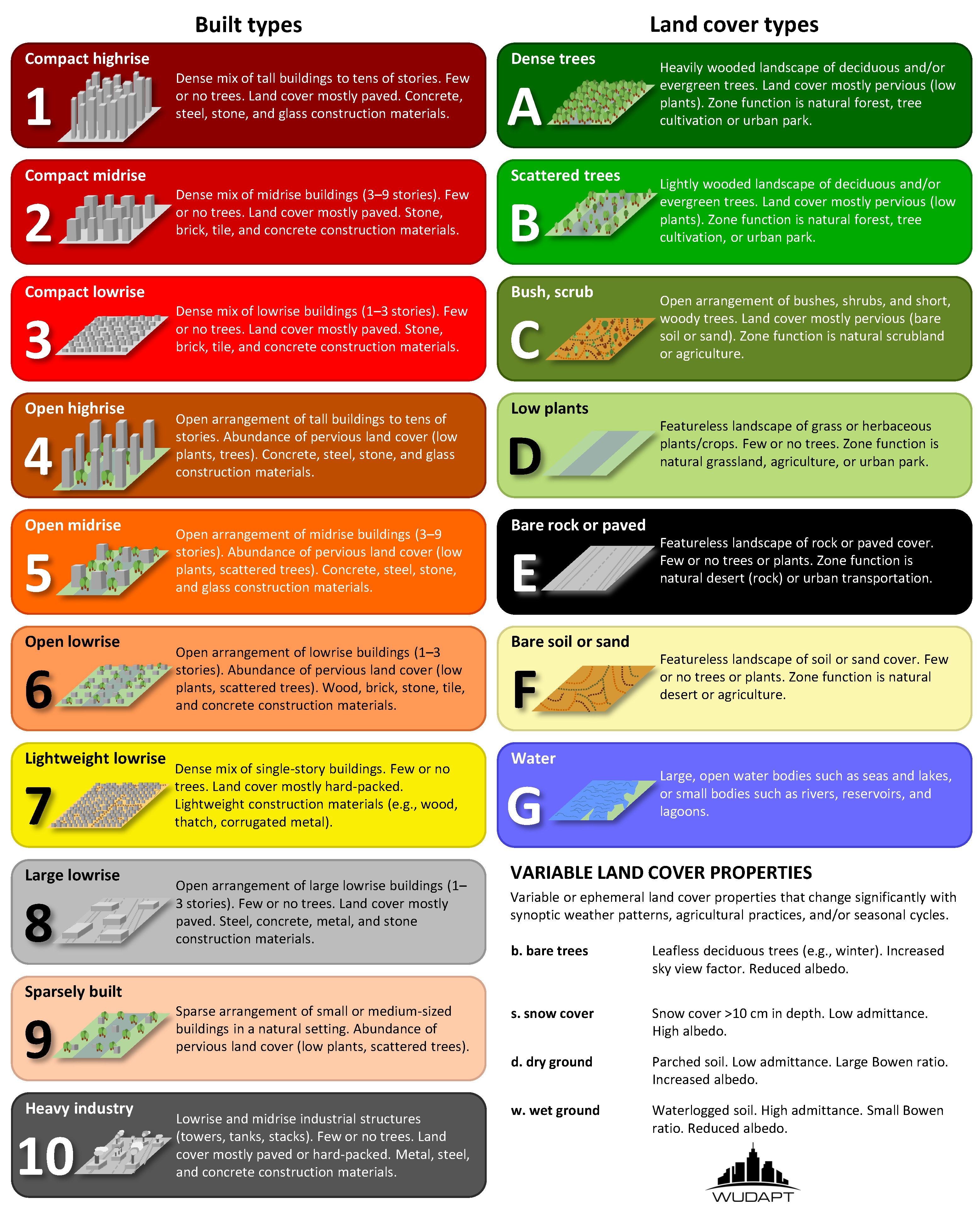
2.3. Local Climate Zones

Local climate zones (LCZs) consist out of 17 types, 10 of which are considered “urban” (Figure 1), and all are associated with characteristic urban canopy parameters (Tables 3 and 4 in Stewart and Oke [23]. In 2015, Bechtel et al. [58] provided a framework to map cities into LCZ maps (lowest level of detail L0 from WUDAPT [27,59,60]) using freely available earth observation data and open-source software. Here, the LCZ mapping procedure follows Demuzere et al. [25,26,28], applying Google’s Earth Engine [61] random forest (RF) classification algorithm [62] on a variety of earth observation datasets (

Table A1. Earth observation (EO) input used in the Local Climate Zone mapping procedure. All EO tiles are retrieved between 1 January 2018 and 31 December 2019, using Google Earth Engine. Most input features are also used in Demuzere et al. [28]; if not, additional references are provided.

Sensor	Band/Ratio
Landsat 8	- Median composites for B2 (red), B3 (green), B4 (red), B5 (Near infrared), B6/7 (Shortwave infrared 1/2), B10/11 (Thermal infrared 1/2)
	- Median composites for the Normalized Difference Vegetation Index (NDVI), the Biophysical Composition Index (BCI), the Normalized Difference BAreness Index (NDBAI), the Enhanced Built-up and Bare land Index (EBBI), the Normalized Difference Water Index (NDWI), and the Normalized Difference Built Index (NDBI).
	- 10th and 90th percentile composites for NDVI and BCI
Sentinel 1	- Single co-polarization (VV), dual-band cross-polarization (VH) and their ratio (VV/VH)
	- Mean and standard deviation of VV and VH combined
	- VVH indicator [103]
Sentinel 2	- Median composite Red edge bands (B5, B6, B7)
	- Median composite NDVI Red Edge 1 and 2 [104]
	- Median composite Sentinel-2 Red-Edge Position Index (S2REP) [105]
Other	- Global Forest Canopy Height (GFCH)
	- DTM, DEM, DSM

). The model is trained using a set of training areas (polygons, hereafter referred to as TAs) that are digitised using Google Earth images [58]. These TAs were gathered by Samsonov and Trigub [38] in a previous effort to map Moscow into LCZs. Yet as the spatial extent of their LCZ map does not cover the full COSMO domain, this effort was repeated to cover the full COSMO model domain. The resulting LCZ map is evaluated in a bootstrapping manner according to Bechtel et al. [59]. Twenty-five different random forests are trained, applied, and evaluated, each using $70\%$ of the TAs for training (stratified by class) and the remaining $30\%$ for testing. For each bootstrap, the following accuracy measures are used: the overall accuracy (OA), the overall accuracy for the urban LCZ classes only (OA${}_u$), the overall accuracy of the built versus natural LCZ classes only (OA${}_{bu}$), the weighted accuracy (OA${}_w$), and the class-wise F1 values. For more details on these accuracy measures, please see Bechtel et al. [63,64].

2.4. LCZ-Based Urban Canopy Parameters

Urban canopy parameter values, sourced from Stewart and Oke [23] and Stewart et al. [65], are assigned to each LCZ class (see

Table A2. Urban canopy parameters per LCZ class, compiled from Stewart and Oke [23] and Stewart et al. [65], including the impervious area fraction (ISA), annual-mean anthropogenic heat flux (AHF), building area fraction (R), building height (H), and height-to-width ratio ($H/W$).

LCZ Class	ISA [unit fraction]	AHF [W/m${}^2$]	R [Unit Fraction]	H [m]	$\mathit{H}/\mathit{W}$ [Unit-Less]
1	0.95	100	0.5	25	2.5
2	0.9	35	0.5	15	1.25
3	0.85	30	0.55	5	1.25
4	0.65	30	0.3	25	1
5	0.7	15	0.3	15	0.5
6	0.6	10	0.3	5	0.5
7	0.85	30	0.8	3	1.5
8	0.85	40	0.4	7	0.2
9	0.3	5	0.15	5	0.15
10	0.55	100	0.25	8.5	0.35

and

Table A3. Radiative and thermal urban canopy parameters per LCZ class, compiled from Stewart and Oke [23] and Stewart et al. [65]. The latter paper only provides thermal admittance values per LCZ class, yet their underlying facet heat conductivity and capacity values are provided by Scott Krayenhoff (pers. communication) and are reported here.

LCZ	Albedo, $\mathit{\alpha }$			Emissivity, $\mathit{ϵ}$			Heat Capacity, ${\mathit{C}}_{\mathit{v}}$			Heat Conductivity, $\mathit{\lambda }$
Class	[Unit Fraction]			[Unit Fraction]			[MJ m${}^{-3}$ K${}^{-1}$]			[W m${}^{-1}$ K${}^{-1}$]
	Roof	Walls	Road	Roof	Walls	Road	Roof	Walls	Road	Roof	Walls	Road
1	0.13	0.25	0.14	0.91	0.9	0.95	1.8	1.8	1.75	1.25	1.09	0.77
2	0.18	0.2	0.14	0.91	0.9	0.95	1.8	2.67	1.68	1.25	1.5	0.73
3	0.15	0.2	0.14	0.91	0.9	0.95	1.44	2.05	1.63	1.0	1.25	0.69
4	0.13	0.25	0.14	0.91	0.9	0.95	1.8	2.0	1.54	1.25	1.45	0.64
5	0.13	0.25	0.14	0.91	0.9	0.95	1.8	2.0	1.5	1.25	1.45	0.62
6	0.13	0.25	0.14	0.91	0.9	0.95	1.44	2.05	1.47	1.0	1.25	0.6
7	0.15	0.2	0.18	0.28	0.9	0.92	2.0	0.72	1.67	2.0	0.5	0.72
8	0.18	0.25	0.14	0.91	0.9	0.95	1.8	1.8	1.38	1.25	1.25	0.51
9	0.13	0.25	0.14	0.91	0.9	0.95	1.44	2.56	1.37	1.0	1.0	0.55
10	0.1	0.2	0.14	0.91	0.9	0.95	2.0	1.69	1.49	2.0	1.33	0.61

for a full list of variables and corresponding values). Thermal and radiative properties are provided on a facet-level (roof, wall and road) and are further averaged over all facets according to Wouters et al. [36]. Afterwards, the resulting UCP values are aggregated to the coarser CCLM model grid. These two procedure are performed with the novel WUDAPT-to-COSMO tool (see Appendix D). For ISA and AHF, the high resolution pixels (100 m) are averaged while being remapped. For all other UCPs, an ISA-weighted mean is applied, in order to conserve the city’s characteristics after remapping to coarser resolution [66]. This procedure is in line with Zonato et al. [34], who have found that a weighted average interpolation performs better than the majority approach that was originally developed in W2W [33].

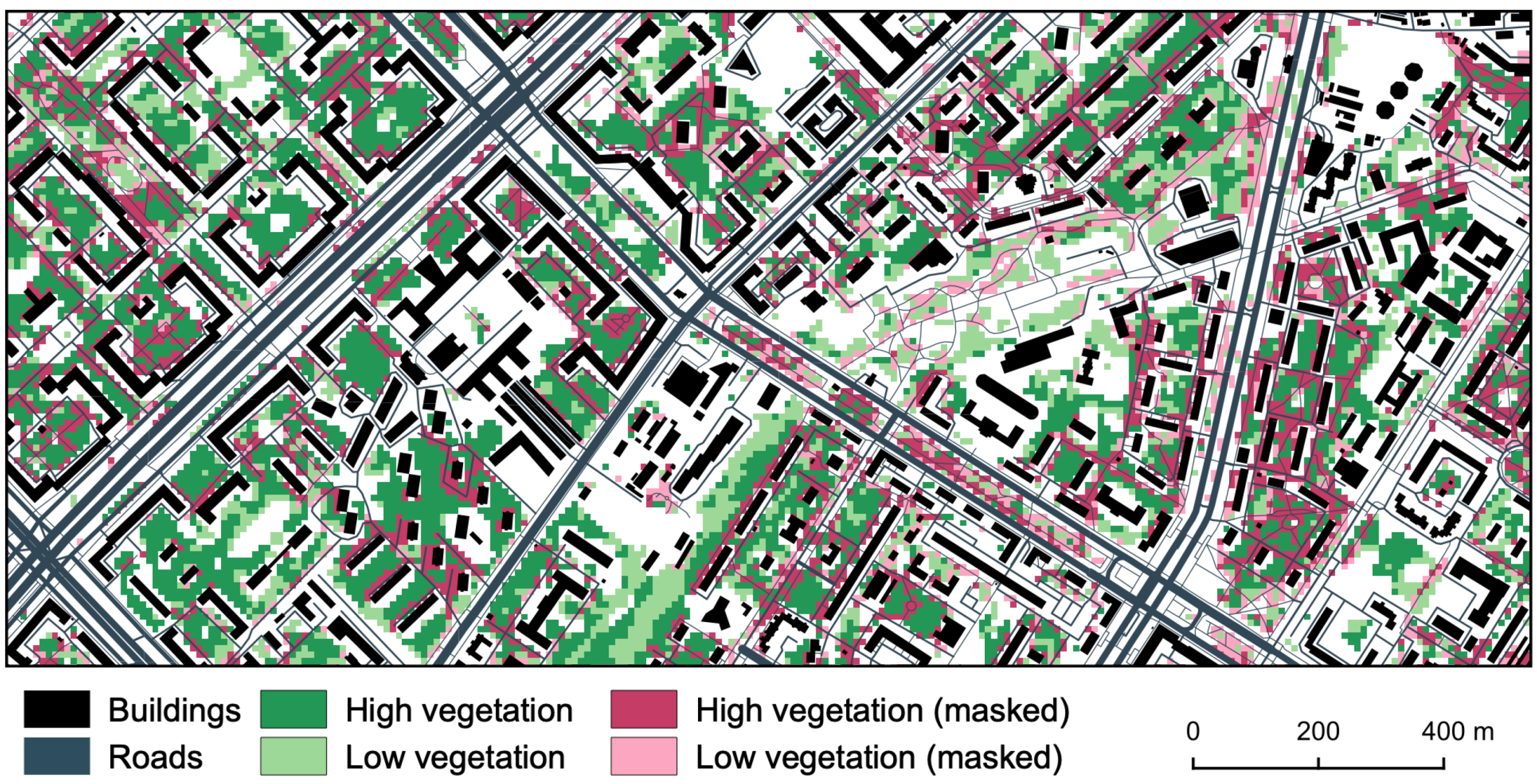
2.5. Reference Urban Canopy Parameters

Reference data for the UCPs (hereafter referred to as REF), are compiled to provide the most realistic description of the Moscow urban environment. REF UCPs are sourced from three independent data sources—land cover data from the recent 100 m resolution Copernicus Global Land Cover (CGLC) dataset [67], vector OpenStreetMap (OSM) data on buildings, roads and land use polygons, and vegetation data derived from 10 m resolution Sentinel-2 satellite images, using a NDVI (Normalized Difference Vegetation Index) threshold value of $0.6$. As the GIS-based approach developed to generate the reference UCPs is detailed in Samsonov et al. [68], only a brief summary is provided here.

The ISA field is determined based on the built-up area fraction from the CGLC data, adjusted for vegetation and OSM data. The CGLC built-up area fraction includes urban vegetation, whereas TERRA_URB assumes no vegetation in the urban tile. Hence, it is assumed that ISA cannot exceed the un-vegetated fraction of the grid cell and cannot be less than the fraction of roads and buildings known from OSM data. A noticeable uncertainty of such estimate appears when the pixels of the 10 m resolution vegetation raster intersect with OSM polygons of buildings and roads, for example, where trees cover paved surfaces (Figure 2). Pixels with such intersections may be considered as a part of paved or vegetated tiles, which gives an uncertainty of ISA values to tens of %. In order to take such uncertainty into account, we consider two versions of the reference dataset, namely REF1 and REF2, where the intersections are considered as unpaved or paved respectively.

Morphological UCPs are determined based on OSM data. The building height H is derived from the number of storeys, even though the latter is only known for $20\%$ of buildings within the study area. Missing values (typically private houses, garages and other small buildings) are derived using an empiric relation between building footprint and number of storeys [68]. The street canyon width W is estimated analytically assuming that the buildings have a square shape and are regularly distributed within the built-up area determined by CGLC. Such approach shows a reasonable agreement with a previous more time-consuming approach identifying street widths in a real built environment [17]. The building fraction R is determined with respect to the CGLC built-up area fraction. The datasets, used in the reference approach, do not provide any evident opportunity to define the thermal parameters. So, we take their constant facet-level values (for road, walls and roof) as means over the dominant LCZs in Moscow (LCZ4 and LCZ5) and calculate the mean thermal parameters for each grid cell in a same way as in LCZ-based approach. The annual-mean AHF is defined based on a Stewart and Kennedy (2017) [69], who suggest an annual mean value of 52 W/m${}^2$ within the administrative borders of Moscow (excluding the “New Moscow” area). To obtain a detailed spatial pattern on a 1 km grid, this value was “weighted” by the product of H and R. Despite the evident simplicity, this approach proved itself in the previous modelling studies for Moscow [6,39,43].

2.6. Model Setup and Study Periods

The COSMO model setup used in the study includes two nested domains with a grid spacing of 3 and 1 km, centred around Moscow. The outer and inner domains sizes were $720\times 720$ km and $200\times 200$ km respectively (Figure 3a). 50 vertical levels were used for both nests. The ICON analysis with a grid spacing of $13$ km was used as initial and boundary conditions for the outer domain, that in turn forced the inner domain. The simulations were performed for two summer and one winter periods:

• 5–25 August 2017, a typical period of relatively warm summer weather that followed after a cold and moist July 2017.
• 1–30 June 2019 with dominant warm and dry weather, higher temperatures than in August 2017, and a high monthly-averaged UHI intensity.
• 1–31 January 2017, a winter period with diverse weather conditions, including extreme cold temperatures on 7–10 January that were accompanied by the development of an intense winter UHI [70].

Initialised in the beginning of each period, the model continuously ran until the end of the period, forced by regularly updated boundary conditions. The first 2 days of each period were considered as a model spin up and removed from analysis. Neither data assimilation nor spectral nudging was applied.

The model options were selected based on previous modelling efforts for Moscow [6,39,43,50] as well as on a number of preliminary simulations for considered periods using the same model version and settings (results not shown). Selected model set up accounts for recent developments in the physical parameterizations, for example, so-called new ICON-based physics [71], Tegen aerosol climatology [72], exponential vertical profile of root density, and a new formulation for bare soil evaporation and vegetation-skin temperature [73]. The revised parameterization of the boundary layer vertical diffusion in the ICON-based physical package, together with the skin-layer temperature formulation, allowed to significantly decrease the nocturnal temperature bias, a characteristic feature of older model versions [6,74,75]. Additional model tuning included a decreased sub-grid thermal homogeneity (from 750 m to 100 m), and the introduction of a scaling factor ($2.5$) for the rooting depth. The latter was applied in order to eliminate the warm and dry bias that typically appears during the hot and dry summer periods. In TERRA look-up tables the rooting depth does not exceed 1 m even for the forests, which is a significant underestimation in comparison to observations [76,77,78]. Previously, a positive effect of the increased rooting depth on the COSMO model biases was found for tropical Africa [79] as well as for the Moscow region [39]. The most important model settings are listed in the Supplementary Table S1.

The TERRA_URB scheme was applied only for the inner model domain. For each considered period, we performed 7 model simulations with different UCP data for TERRA_URB (

Table 1. Summary of the urban canopy parameters (UCPs) datasets, used in numerical experiments.

Name	ISA		AHF	Morphological UCPs	Thermal UCPs
	2D field		2D field
DEF	from EXTPAR [56]		from EXTPAR [53]	Constants from Reference [36]	Constants from Reference [36]
LCZa			LCZ-based 2D fields		Constants from Reference [36]
LCZb					LCZ-based 2D fields
REF1a	2D field based	less paved	2D field based		Constants from Reference [36]
	on CGLC, OSM	fraction	on estimate from [69]	2D field based	2D field based
	and Sentinel imagery		and OSM data	on OSM data	from facet-level
REF1b					constants
REF2a		more paved			Constants from Reference [36]
		fraction			2D fields derived
					from facet-level
REF2b					constants

). The DEF simulation uses default ISA and AHF fields from EXTPAR and hard-coded morphological and thermal UCPs from Wouters et al. [36], and serves as a baseline. The LCZa, REF1a and REF2a simulations use 2D fields of ISA, AHF and morphological UCPs obtained by the LCZ-based and reference approaches, while the thermal parameters remain constant (as in DEF). 2D fields of thermal UCPs were incorporated in LCZb, REF1b and REF2b simulations. We further use the * symbol to refer to a group of simulations (e.g., REF* means all REF1a, REF1b, REF2a, REF2b simulations). For all model simulations with TERRA_URB, additional external parameter processing steps were performed in order to resolve the inconsistencies between the default land surface description based on Globcover and the new UCPs (see Appendix C for details).

Our experimental setup aims at answering the following research questions:

• What is the modelled impact of using advanced UCPs compared to baseline settings?
• Which ISA calculation (REF1/REF2) is better?
• Does the LCZ scheme provide a valid alternative for REF UCPs?
• What is the added value of the LCZ-based thermal UCPs?

2.7. Observations for Model Verification

To evaluate the model performance, we use regular observations from a dense meteorological network (Figure 3) which consists of weather stations (WSs) of the Russian hydrometeorological service (Roshydromet) and automatic air-quality stations (AAQS) of Mosecomonitoring, Moscow’s official environmental monitoring service. The WSs provide the most reliable data, however only a few stations are available in urban areas: the Balchug WS in the city center, the meteorological observatory of the Lomonosov Moscow State University (MSU), VDNKh WS in an urban park, and several WSs in the suburbs. AAQSs covers the city with a denser network, but provide less accurate data that should be used with a caution. Meteorological observations by AAQSs do not comply with the standards of the World Meteorological Organization (WMO), for example, the sensors may be located at a height of 2 m above roofs or metal containers, and 4 m above the ground (instead of WMO’s $1.5$ to 2 m above ground level). Previous studies showed that AAQS temperature measurements may be biased during daytime, however the daily-mean and nighttime temperatures are accurate enough for spatially-explicit UHI and model verification studies [43,80]. We use the data on 3-hourly intervals from 37–42 WSs and 39–40 AAQSs (the number of stations varies due data availability and quality for the considered periods).

In order to take into account coordinate uncertainties and potential discrepancies between the land-cover data in the model grid cells and in the actual location of the observational sites, we propose an advanced routine for model-to-observation comparison. The model grid cell for a comparison with a specific WS or AAQS is selected among its 4 nearest neighbours, by minimising the temperature RMSE. In addition, the selected model grid cell should have a similar degree of urbanisation compared to its corresponding station. This similarity is defined in terms of three simple categories: natural, mixed and dense urban. Since the stations are typically located over grass or lawns, we take a value for natural model tile for a comparison with observations, excepting a few WSs and some AAQS located in a dense urban environment. For the latter, a grid-cell-averaged modelled values are further used.

2-meter air temperature and its urban-rural difference, known as UHI intensity (UHII), are selected as key variables for model verification and analysis. Observed and modelled UHII is defined in line with previous studies for Moscow [6,39,43,80] as a temperature anomaly with respect to the mean rural temperate, averaged over 9 stations around Moscow (Klin, Dmitrov, Alexandrov, Pavlovsky Posad, Kolomna, Serpukhov, Maloyarslavets, Naro-Fominsk, Novo-Ierusalim, see Figure 3a).

3. Results

3.1. Local Climate Zone Map

The average overall accuracies over all bootstraps vary between $65\%$ (OA${}_u$) and $98\%$ (OA${}_{bu}$), well above the defined threshold of $50\%$, defined by Bechtel et al. [59] to pass the automated quality control process (results not shown). The final LCZ map (Figure 3) is obtained by training the classifier on all available TAs, and is exported with a spatial resolution of 100 m. As single pixels do not constitute an LCZ class, and granularity is often present in the raw LCZ maps, the raw LCZ maps are post-processed using a Gaussian kernel majority filter [26]. Finally, since we are only interested in the urban heterogeneity and not the natural LCZ land covers, all non-urban LCZs are masked using the Global Artificial Impervious Area (GAIA) product for the year 2015 [81] (Figure 4b).

3.2. Urban Canopy Parameters

Comparison between DEF, LCZ and REF UCPs reveals noticeable differences. For ISA, such comparison also included the aforementioned globa CGLC and GAIA data sets. The DEF dataset extracted from EXTPAR demonstrates the smoothest and least realistic ISA spatial pattern (Figure 4c). This is not surprising since the ISA data in EXTPAR is derived from the coarser resolution (30-second) LandScan population density data [56]. The LCZ-based and REF ISA estimates resolve the shape of the megacity and interurban alternation of parks and built-up areas much better. These datasets have almost similar spatial patterns, but still differ in ISA magnitude. The LCZ-based values are the lowest (Figure 4d) with a mean city/city-center value of $50\%$/$69\%$ (

Table 2. UCP values for DEF, LCZ and REF, averaged within the major part of the city (within Moscow administrative borders for the year of 2011, that approximately corresponds to Moscow Ring Road) and within the central part of the city (within a distance of 5 km from Kremlin, that approximately corresponds to Third Ring Road). For the morphological and thermal UCPs in LCZ and REF, the values are weighted by ISA when averaging.

UCPs	Unit	DEF		LCZ		REF1/REF2
		City	Center	City	Center	City	Center
ISA	%	89	100	50	69	50/58	81/87
AHF	W/m${}^2$	51	69	28	22	52	88
Building fraction, R	%	66.7		33.1	38.1	19.1	26.9
Building height, H	m	15		18.6	17.1	21.5	18.2
Canyon height-to-width ratio, [$H/W$]	unit-less	1.5		0.75	0.86	0.54	0.69
Facet-level albedo, $\alpha$	unit fraction	0.101		0.175	0.177	0.178	0.175
Facet-level emissivity, $ϵ$	unit fraction	0.86		0.917	0.916	0.922	0.918
Facet-level heat capacity, $C_v$	MJ m${}^{-3}$ K${}^{-1}$	1.25		1.789	1.910	1.762	1.791
Facet-level heat conductivity, $\lambda$	W m${}^{-1}$ K${}^{-1}$	0.767		1.104	1.142	1.024	1.061

). The REF1 dataset (Figure 4e) provides a similar city-mean value but a higher mean city-center value of $81\%$. REF2 dataset (Figure 4e) is compiled taking less vegetated area into account (Figure 2), so the corresponding mean values are $58\%$ (city) and $87\%$ (city-center). Despite the differences between LCZ-based and REF datasets, they are more realistic in comparison not only to the DEF data, but also to the more recent CGLC and GAIA global datasets (Figure 4a,b), two potential candidates to replace the current ISA data in EXTPAR. While CGLC represents the built up area fraction, and GAIA ISA, both products return $100\%$ of ISA/built up area for the major part of the city, including the vegetated residential areas outside of the center (typically LCZ4 and LCZ5). This is not surprising for CGLC, since its built up land cover class includes urban vegetation. For GAIA however, ISA values seem to be strongly overestimated.

The annual-mean AHF values also strongly differ between the considered UCP datasets. The DEF values are derived from Flanner’s (2009) [53] data with $2.5\times 2.5$ min resolution, which is too coarse to resolve the intra-urban heterogeneity (Figure 5a). Moreover, they are not fully consistent with default ISA data. For example, several urban areas around Moscow are represented in the DEF ISA, but are completely missing in the AHF field. Additionally, the AHF maximum is unrealistically shifted to the south-west of the city. The LCZ-based and REF approaches (Figure 5b,c) provide more detailed spatial patterns, but with different magnitudes: the LCZ-based approach provides a mean city/city-center value twice/four times lower compared to the REF approach (Table 2). REF AHF estimates are based on literature data [69], and better agree with independent literature estimates for Moscow [82,83]. LCZ-based AHF values therefore seem underestimated, which is not surprising since the LCZ-based values were originally suggested for cities in more temperate climates, characterised by a lower less heating demand in winter.

The LCZ-based and REF approaches generally agree in their spatial variation of the morphological UCPs, with distinct different characteristics between the historical city center, areas of more modern development (major part of the city) and the suburbs (Figure 6). Differences between these approaches are most noticeable for the building area fraction, R, and canyon height-to-width ratio, $H/W$ (Table 2, Figure 6). The LCZ-based approach generally provides higher R and $H/W$, lower H and lower spatial variability of these parameters. Again this is not surprising, since the LCZ-based values are very generic. In addition, lower R and $H/W$ values in REF may be due to the underestimation of these parameters when the OSM data misses some buildings. Nevertheless, the differences between LCZ and REF UCPs are much less dramatic than the differences with respect to the default values from Wouters et al. [36], used in DEF (Table 2), especially for R and $H/W$ parameters. The difference between DEF and LCZ-based thermal parameters is also noticeable. The latter are characterised by higher albedo, emissivity, heat capacity and conductivity characteristics. Thermal parameters in REF UCPs are also derived using the LCZ-based constants for individual facets, so their city-mean values are in line with the LCZ-based values.

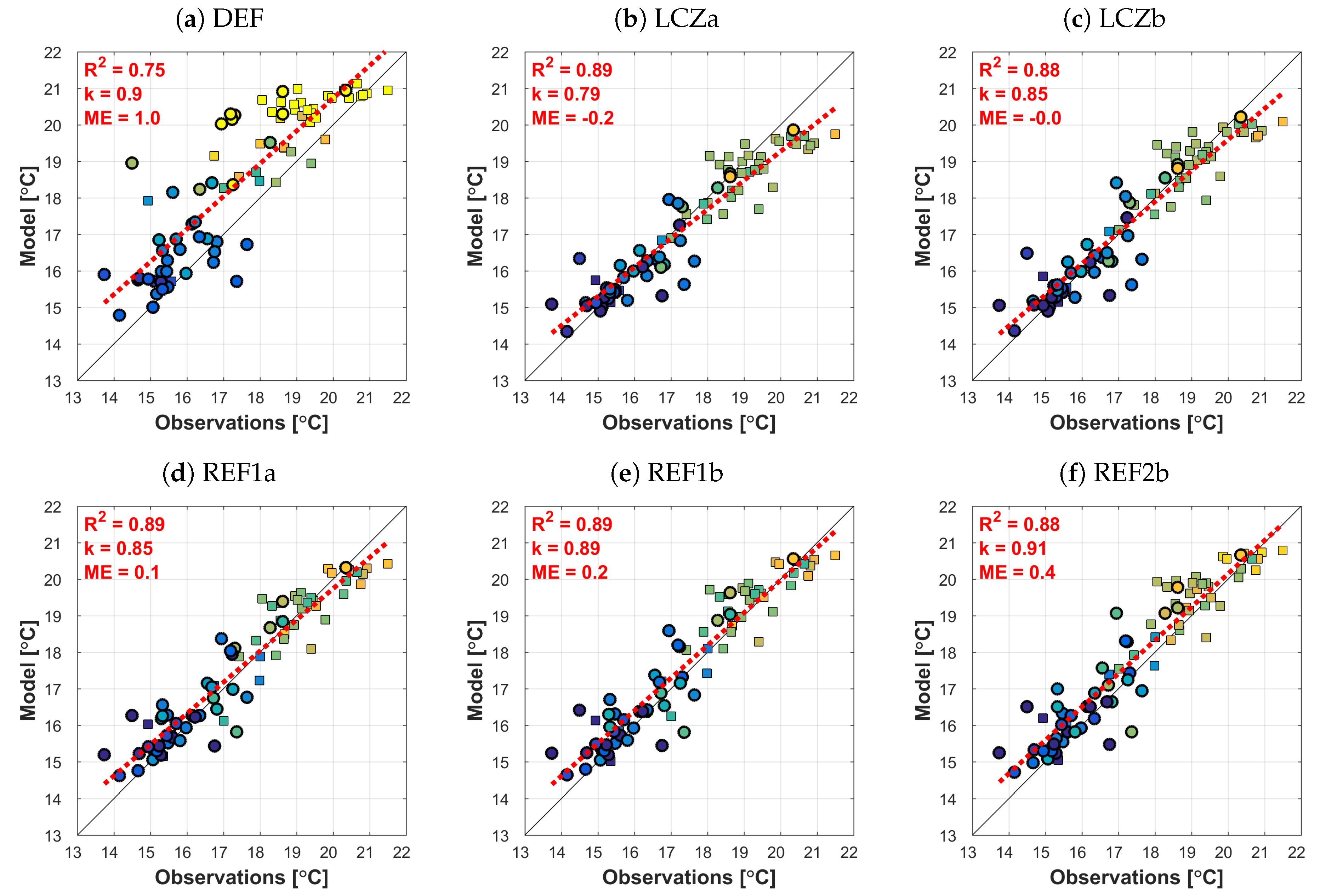
3.3. Model-to-Observation Comparison for Summer Conditions

For both summer periods, the model reasonably reproduces the observed meteorological conditions in Moscow region, including the rural temperature regime. For the period in August 2017 (Figure 7a), the model reproduces rural temperatures with a near-zero mean error (ME), slightly underestimating daily maximum temperatures during the hottest days with a mean daytime (9–12 UTC) error of $-0.4$ ${}^{\circ }$C. As expected, the simulated temperature for rural stations varies very little between the model simulations with different UCPs. For the period in June 2019 (Figure 7c), the model simulates the rural temperature with a mean ME of $0.4$ ${}^{\circ }$C and slightly overestimates the daily temperature range (Figure 8e), resulting in a daytime ME exceeding the nighttime ME ($0.7$ ${}^{\circ }$C and $0.5$ ${}^{\circ }$C respectively). The different model behaviour for two summer periods may be caused by various unaccounted factors related to the soil hydrological processes, initial soil moisture conditions, radiation transfer, and so forth. Further analysis of such factors is beyond the scope of this study, however it is important that two summer periods allow us to evaluate the impact of the UCPs on simulated urban temperatures against a background of different regional-scale model biases.

As in previous modelling studies for Moscow [39,43], the model captures the general patterns of the UHII temporal variations. This is shown for example, for Balchug WS in the city center (Figure 7b,d). All model simulations capture the typical UHII diurnal pattern with a nocturnal maximum close to 8–9 ${}^{\circ }$C, as well as synoptic-scale UHII oscillations driven by weather conditions. For a more in-depth comparison between the model simulations, we selected a set of the sub-periods that represent days with the strongest UHIs, and that exclude days with excessively high temperature error (see cyan boxes in Figure 7).

The panels in Figure 8 show the mean observed and simulated UHII diurnal cycles for selected sub-periods. For the city center (Figure 8b,f), the difference between the model simulations is indeed small, with the lowest UHII for the LCZ simulations and the highest UHII for REF2*. For all simulations, the modelled UHII diurnal cycle for the city center is shifted by phase in comparison to the observations, with a negative/positive ME in the morning/evening. Such phase shift is partially but not fully eliminated in the simulations with LCZ-based thermal parameters (LCZb, REF1b, REF2b). For the urban parks (MSU and VDNKh WSs), the phase shift is less pronounced (Figure 8c,d,g,h). In contrast to urban park WSs, the Balchug Ws is located inside the urban canopy. So, the UHII phase shift for this WS may be partially caused by canopy-layer effects that remain unresolved in bulk UCMs such as TERRA_URB. The differences between the model simulations are higher for urban park Wss, where the baseline DEF simulation strongly overestimate the UHII (especially for VDNKh WS), while the others show a better agreement with observations.

Temperature anomaly maps allow to get a broader perspective on the simulated and observed UHI. Figure 9 presents such maps for nocturnal conditions (21–24 UTC) in August 2017, while the maps for June 2019 are presented in Supplementary Figure S1. Such maps clearly illustrate the dramatic difference between the smooth UHI spatial pattern in DEF and the more detailed patterns in all other simulations: all LCZ* and REF* simulations have similar spatial UHI patterns, with the highest temperatures in the city center, local cool anomalies in urban parks and local hotspots in smaller towns around Moscow. The nocturnal urban temperatures increase when going from LCZ* to REF* simulations, from REF1* to REF2* simulations with higher ISA, and from simulations with default thermal parameters (*a) to simulations with LCZ-based thermal parameters (*b). The spatial patterns of the daily-mean UHII in general follows the nocturnal ones, with the only difference that *b simulations do not increase the daily-mean UHII. Incorporation of the REF1 UCPs instead of the LCZ-based ones increases the city and city-center mean temperatures by approximately $0.3$ ${}^{\circ }$C and $0.6$ ${}^{\circ }$C respectively, while the ISA increase in REF2 additionally increases the city-mean temperatures by $0.2$ ${}^{\circ }$C. Incorporation of the LCZ-based thermal UCPs increases the city-mean nocturnal temperature by about $0.3$ ${}^{\circ }$C and equally decreases the daytime temperature, which is consistent with a decrease in albedo and increase of thermal admittance in the LCZ-based thermal UCPs (Table 2). All pairwise temperature differences between the model simulations are given in Supplementary Table S2.

Scatter plots in Figure 10 show the relationships between the modelled and observed nocturnal temperatures for August 2017. The worst agreement with a trend determination coefficient $R^2=0.74$ is found for DEF. All other simulations depict a similar agreement between the modelled and observed nocturnal temperatures. LCZa, characterised by default thermal UCPs, noticeably underestimates the temperature for the warmest sites in the city center, which gives the lowest slope coefficient $k=0.79$. Other simulations reproduce warmer nocturnal temperatures in the city center, which increases k up to $0.91$ for REF2b. Yet in all cases, k is lower then 1 for nocturnal temperatures, which may be explained by the model’s inability to resolve the coldest and warmest extremes, potentially caused by to sub-grid orography in rural areas and urban canopy layer in the densely built environment respectively. The underestimation of the nocturnal temperature heterogeneity in the model is compensated during the rest of the day, resulting in daily-mean temperature slope coefficients slightly higher than 1 for REF* and DEF, and slightly below 1 for the LCZ* simulations (see Supplementary Figure S2). The plots for June 2019 (Supplementary Figures S3 and S4) demonstrate very similar results, but with an overall lower trend slope for nocturnal and daily-mean temperatures ($k\le 0.85$).

The considered plots and maps illustrate a dramatic difference between DEF and the other simulations, however it is still difficult to judge which one among the LCZ* and REF* simulations is better. In order to support such judgement, we consider the verification scores, namely the mean error (ME) and the root-mean square error (RMSE) for air temperature and UHII. The latter allows to exclude at least a part of the model errors that is not related to urban-atmosphere interactions. In addition to area-mean ME and RMSE scores, we consider the scores for different groups of observational sites: for “rural” sites, located at the distance of more than 25 km from the city center excluding those located within a dense built environment (in total 26–30 WSs and 2–3 AAQSs); “urban” sites within a distance of 25 km from the center including the suburbs and urban park areas (8–11 WSs and 32–35 AAQSs); sites in the central part of the city within a distance of 5 km from the center (only one WS, Balchug, and 6–8 AAQSs). As mentioned previously, it is necessary to be careful with estimates based on the less reliable AAQS data, therefore we also separately consider the verification scores based on WSs and AAQSs. For rural sites, we further consider only WSs. ME and RMSE scores are calculated for temperature and UHII, for different times of the day (all, daytime and nighttime hours), and averaged over different groups of observational sites. All considered scores are presented in Supplementary Tables S3 and S4, while Figure 11 depicts the scores for air temperature and UHII (all times of the day), and for the nocturnal UHII.

Verification scores confirm the strong improvements for LCZ* and REF* simulations over DEF. The area-mean temperature RMSE decreases from $1.6$ ${}^{\circ }$C to approximately $1.3$ ${}^{\circ }$C in August 2017 (by $18\%$) and from $2.05$ ${}^{\circ }$C to $1.8$ ${}^{\circ }$C (by $12\%$) in June 2019. RMSE decreases by more than $30\%$ for urban WSs, both for air temperature and UHII (Figure 11). Among the other simulations, the LCZ* simulations provide as good area-mean scores as the REF* simulations. However, LCZa performs worse than others for the city center due to UHII underestimation for this area by $0.7$ ${}^{\circ }$C in August 2017 and $1.6$ ${}^{\circ }$C in June 2019. In June 2019 with an overall stronger UHI, underestimation of the nocturnal UHII pulls down the mean UHII ME for all day times. The central part of the city is represented by only one WSs and a few AAQSs, so it weakly contributes to the area-mean verification scores. However, we consider the model’s ability to simulate the UHII in this area as an important verification metric. Underestimation of the nocturnal UHII is partially eliminated in LCZb with 2D thermal UCPs as well as in REF* with higher ISA in the city center.

As already noted, incorporation of the LCZ-based thermal UCPs decreases the diurnal temperature range in urban areas. Such effect may be considered as generally positive in terms of verification scores. Comparison of the scores between *a and *b simulations shows that the latter generally provide slightly better or similar verification scores (Figure 11, Supplementary Tables S3 and S4), with the only exception for the daytime UHII in June 2019 (Supplementary Table S4). For June 2019, daytime UHII is already underestimated in *a simulations, and *b simulations further amplify such errors. Such underestimation is not necessary related to UCPs. It may be also caused by an interplay of other processes such as turbulence and radiation transfer. Nevertheless, for June 2019 the *b simulations provide better scores for daytime temperature. Comparison of the scores for REF1* and REF2* simulations with lower or higher ISA, reveals that the latter perform slightly better for the city center (especially for AAQSs), but provide higher temperature and UHII ME for other urban areas. Hence, the higher ISA in REF2 UCP dataset is likely excessive. Finally, based on the balance between different verification metrics, we may conclude that REF1b is likely to provide the best results, however its advantage over other REF* and LCZ* simulations is negligible.

Summing up the results for summer conditions, we can highlight the comparable quality of the modelled urban thermal environment with LCZ-based and reference UCPs, and the huge improvements achieved by incorporation of such advanced UCPs instead of the baseline settings. These results are achieved firstly by providing a detailed and realistic ISA map to the model. This is not surprising since ISA is found to be among the most important UHI drivers for summer season [84,85,86]. The other UCPs are also important, but it is difficult to trace their impact on the model verification scores based on the available canopy-layer observations.

3.4. Model-to-Observation Comparison for Winter

Winter temperature and UHII dynamics in Moscow dramatically differ from summer conditions. Due to the presence of snow cover, short sunlight duration and low solar incidence angles (not more that ${13}^{\circ }$ in January), the temperature and UHII diurnal cycles are almost absent in December and January, and their variations are mostly determined by the alteration of synoptic conditions. As in summer, the strong wintertime UHI is observed under calm, clear and often frosty weather. Such pattern of the wintertime UHI dynamics is typical for other cities with cold winters, for example, Lodz (Poland, [87]) and a number of Russian Arctic cities [88,89].

The considered winter period of January 2017 is characterised by a variety of weather conditions and includes three episodes with intense UHIs (Figure 12). The first episode was observed on a background of extreme frosts between 7–11 January (see detailed case study analysis in [70]), and the two shorter episodes were observed later that month around the 17th and 26th of January. The model reasonably reproduces the observed variations of the rural temperature, including its rapid drops and the lowest extremes (Figure 12a). All model simulations with different UCPs reproduces the basic patterns of the UHII variations, with its peaks during the three listed episodes (Figure 12b). DEF and REF simulations provide almost similar UHII dynamics for city center and capture the observed UHII extremes, but LCZ* simulations reproduce noticeably lower UHII and underestimate its peaks by 1–3 ${}^{\circ }$C. As for summer, subsequent analysis are performed for the three periods with an intense UHI (cyan boxes in Figure 12).

The temperature anomaly maps in Figure 13 illustrate the UHI spatial patterns for these episodes, and scatter-plots in Figure 14 provide more in-depth information on the model-to-observations comparison. For winter conditions, the difference between model simulations with default and LCZ-based thermal UCPs is negligible, as well as a difference between REF1* and REF2* simulations with lower or higher ISA. Therefore, for clarity, we present the results only for DEF, LCZb and REF1b. The UHI maps and scatter-plots clearly illustrate that LCZ simulations strongly underestimate the UHII for the whole city, while DEF and REF simulations reproduce more realistic UHII values. Such results are consistent with the AHF differences between the UCP datasets. The city-mean values in REF and DEF UCPs are almost similar, while the LCZ-based estimate is half their value (see Table 2). On average, LCZ* model simulations produce an UHI that is $40\%$ less intense than DEF and REF*, and $50\%$ less than the observed one. This result confirms the previous findings on the dominant role of AHF in winter for the UHI generation in mid- and high-latitude cities [89,90,91].

As for the summer, the REF and LCZ simulations provide more detailed spatial UHI patterns compared to the DEF simulation. However, there are only minor differences between the DEF and REF simulations in terms of verification scores, with a similar $R^2$ (≈0.9)) and slightly better ME and RMSE scores for REF for temperature and UHII (see Supplementary Tables S3 and S4). Such result may indicate that the AHF map in the REF UCP data, despite the detail, is far from being perfect and needs to be improved further.

4. Discussion and Conclusions

The presented study compared three approaches to obtain urban canopy parameters (UCPs) for atmospheric mesoscale modelling using the COSMO model and the TERRA_URB urban canopy scheme for the Moscow megacity. The currently-used default urban description in COSMO, based on global datasets and hard-coded constants, was selected as a baseline (DEF UCPs). Secondly, a new WUDAPT2COSMO tool was developed to define the required UCPs in the framework of the World Urban Database and Access Portal Tools (WUDAPT) project [27], based on Local Climate Zones (LCZs) and LCZ-specific UCP constants from Stewart and Oke (2012) [23] and Stewart et al. [65] (LCZ UCPs). Finally, the best available reference urban description was compiled with a new comprehensive GIS-based approach [68] based on OpenStreetMap data, recent CGLC [67] global land cover data and Sentinel-2 satellite imagery (REF UCPs). High-resolution simulations with these UCPs on a 1 km${}^2$ grid were performed for contrasting summer and winter periods and evaluated against a dense observational network. Results of the study demonstrate the importance of the UCPs for the megacity’s modelled thermal environment and high potential for model improvements by providing more detailed, reliable and consistent UCPs. Specifically, the following conclusions can be inferred:

• The currently-used default urban description in COSMO and its EXTPAR tool is based on outdated global datasets and hard-coded constants. This description is too distant from the realistic and detailed urban description required for high-resolution weather and climate modelling, and needs to be improved.
• The noticeable improvements of the model evaluation scores may be achieved by providing more detailed and realistic UCPs. In our study, incorporating advanced LCZ-based and REF UCPs allowed to decrease the summertime RMSE for temperature and UHI intensity for urban areas and suburbs by up to $30\%$ in comparison to the baseline DEF simulations.
• The simulations with LCZ-based and REF UCPs demonstrated almost similar evaluation scores for the summer season. This is in line with previous studies that evaluated simulations with LCZ-based UCPs with another model, WRF, and for other cities [30,33]. The LCZ-based approach worsened model performance for winter, which is due to the underestimation of the anthropogenic heat flux. This issue may be solved by introducing a simple scaling coefficient or by revising the LCZ-specific constants in future research.
• An important advantage of the LCZ-based approach lies in a possibility to define thermal parameters of urban materials. Replacing the default constants sourced from [57] by the LCZ-based values additionally provides a minor, but noticeable model improvement, for both the LCZ and REF UCP simulations. And while such improvements are not always clearly visible from the model verification scores due to an interplay of other sources of model errors, the LCZ-based thermal parameters nevertheless improve the representation of the diurnal temperature cycle and daily temperature range.
• For the GIS-based approach, better results are achieved if the intersections between the pixels of the Sentinel-derived vegetation raster and vector polygons of impervious surfaces (buildings and roads) are interpreted as vegetated unpaved areas.

The LCZ and GIS-based approaches considered here are both promising for providing detailed and consistent UCPs for urban weather and climate modelling in COSMO (and ICON in the future). The GIS-based approach is more realistic, however, it is not devoid of inaccuracies associated with incomplete OSM records or ISA estimation uncertainties. Both approaches are based on the globally-available data and may be applied for other study regions. However, the LCZ-based approach is evidently simpler and better suited as universal solution. The GIS-based approach requires data collection from different sources and is computationally expensive, and labour-demanding, while the LCZ-based approach requires only a LCZ map. The LCZs nowadays become a standard surface descriptor for urban climate studies, so such maps are already created for many world’s cities and uploaded to the WUDAPT portal [92]. Moreover, an online LCZ-generator is currently under development providing an online tool that maps a city of interest into LCZs, solely expecting a valid training area file and some metadata as input [93]. Thus, the LCZ-based approach may be recommended as an effective tool to get a first-order approximation of the UCPs on a wide range of scales, which may be further used directly to run the model or as an additional data source to supplement more advanced techniques as suggested in [19]. At the same time, the proposed GIS-based approach may be recommended for more comprehensive limited-area model applications.

The LCZ-based approach is promising for providing the UCPs on a continental or even global scale. Continental LCZ maps already exist for Europe [28] and the continental United States [26,94], both paving the way for global coverage. Such advancement is especially important for the ICON model, which will replace the COSMO model in COSMO NWP consortium and CLM-Community as a seamless tool for global and limited-area applications [51,52]. The ICON model does not include any UCM yet, however there are plans to transfer the TERRA_URB scheme from COSMO to ICON in a near future. To support urban applications with COSMO/ICON models, we suggest that WUDAPT2COSMO tool should be embedded in EXTPAR, allowing the user to choose the LCZ-based approach directly when extracting the external parameters.

Presented results allow making more general conclusions with respect to the further UCMs and UCPs development. In our study, a huge improvement of the model verification scores for summer was achieved firstly by providing a realistic ISA map. This result confirms the ISA importance as a driver of the summertime urban thermal environment [84,85,86]. Considered REF and LCZ approaches not only improve ISA detail, but provide substantially lower ISA values in comparison to model’s default urban description [56] and more recent global GAIA data [81]. Actual ISA values are also lower than the built up area fraction from GGLC [67] and other land cover datasets such as Globcover2009 [55]. The later is not surprising since the urban or built up land cover classes include urban vegetation. However, unresolved urban vegetation and excessively high ISA values in datasets such as GAIA should be considered as potential limitations. Additionally, there is room for improving the model’s representation of the vegetated urban areas. Currently, TERRA_URB assumes that the urban tile is completely impervious, while the vegetated area is virtually moved outside the urban canopy. Such simplification may cause an underestimation of the urban canopy impacts on the surface-atmosphere interaction, for example, on the surface roughness. This problem is typical not only for TERRA_URB, but also for more comprehensive UCMs such as DCEP in COSMO [95] and various schemes in WRF [96,97]. On the other hand, several studies have already demonstrated the noticeable impacts of explicitly accounting for urban vegetation in UCMs [98,99]. Thus, our study highlights the importance of the accurate ISA definition taking into account urban vegetation, and calls for more attention to urban vegetation in further UCM developments.

For the first time, TERRA_URB in COSMO was comprehensively evaluated for cold winter conditions. As expected, the model demonstrated a strong sensitivity to the AHF and low sensitivity to the ISA and thermal UCPs. Despite the oversimplified AHF parameterization in TERRA_URB with a pre-defined annual cycle, the model successfully captured the wintertime UHI in REF* and DEF* simulations with almost similar city-mean AHF, and underestimated the UHII by approximately $50\%$ in LCZ* simulations which are characterised by only half of the city-mean AHF. This is expected since the LCZ-specific AHF constants were suggested by Stewart and Oke [23] for more temperate cities with warmer winters and less heating demands. Surprisingly, more detailed AHF map in REF* simulations provided only minor improvements over DEF with a much coarser AHF data, which indicates the imperfectness of the AHF spatial patterns in both datasets. This result underlines the importance of detailed and representative AHF information in order to improve the model’s performance in winter. Future efforts may thus include a revision of the LCZ-specific AHF constants taking into account regional features, the examination of new global AHF datasets, for example, [100,101], and the application of comprehensive AHF models such as the large scale urban consumption of energy (LUCY) model [102].

Finally, the limitations of the presented study should be mentioned. Despite the noticeable differences in the morphological UCPs between DEF, REF and LCZ datasets, our study does not allow judging about their particular importance for the modelling results. In part, this is due to the relatively low model sensitivity to their changes, noted earlier in [36]. Such sensitivities may be higher for more comprehensive UCMs that explicitly resolve the urban canopy layer. Presented conclusions on the advantages and shortcomings of the considered UCP datasets in some cases are supported by only minor differences in the model verification scores. In further studies they should be supported by involving additional data for model verification, for example, the observations on other meteorological variables (wind speed and air humidity) and remotely-sensed land surface temperature products.

References

1. Oke, T.R.; Mills, G.; Christen, A.; Voogt, J.A. Urban Climates; Cambridge University Press: Cambridge, UK, 2017; pp. 1–16. [Google Scholar] [CrossRef] [Green Version]
2. Tanner, C.J.; Adler, F.R.; Grimm, N.B.; Groffman, P.M.; Levin, S.A.; Munshi-South, J.; Pataki, D.E.; Pavao-Zuckerman, M.; Wilson, W.G. Urban ecology: Advancing science and society. Front. Ecol. Environ. 2014. [Google Scholar] [CrossRef]
3. Fernandez Milan, B.; Creutzig, F. Reducing urban heat wave risk in the 21st century. Curr. Opin. Environ. Sustain. 2015, 14, 221–231. [Google Scholar] [CrossRef] [Green Version]
4. Baklanov, A.; Grimmond, C.; Carlson, D.; Terblanche, D.; Tang, X.; Bouchet, V.; Lee, B.; Langendijk, G.; Kolli, R.; Hovsepyan, A. From urban meteorology, climate and environment research to integrated city services. Urban Clim. 2018, 23, 330–341. [Google Scholar] [CrossRef]
5. Baklanov, A.; Cárdenas, B.; Lee, T.C.; Leroyer, S.; Masson, V.; Molina, L.T.; Müller, T.; Ren, C.; Vogel, F.R.; Voogt, J.A. Integrated urban services: Experience from four cities on different continents. Urban Clim. 2020, 32, 100610. [Google Scholar] [CrossRef] [PubMed]
6. Rivin, G.S.; Rozinkina, I.A.; Vil’fand, R.; Kiktev, D.B.; Tudriy, K.O.; Blinov, D.V.; Varentsov, M.; Zakharchenko, D.I.; Samsonov, T.; Repina, I.A.; et al. Development of the High-resolution Operational System for Numerical Prediction of Weather and Severe Weather Events for the Moscow Region. Russ. Meteorol. Hydrol. 2020, 45, 455–465. [Google Scholar] [CrossRef]
7. Barlage, M.; Miao, S.; Chen, F. Impact of physics parameterizations on high-resolution weather prediction over two Chinese megacities. J. Geophys. Res. Atmos. 2016, 121, 4487–4498. [Google Scholar] [CrossRef] [Green Version]
8. Vandamme, S.; Demuzere, M.; Verdonck, M.l.; Zhang, Z.; Coillie, F.V. Revealing Kunming’s (China) Historical Urban Planning Policies Through Local Climate Zones. Remote Sens. 2019, 11, 1731. [Google Scholar] [CrossRef] [Green Version]
9. Verdonck, M.L.; Demuzere, M.; Bechtel, B.; Beck, C.; Brousse, O.; Droste, A.; Fenner, D.; Leconte, F.; Van Coillie, F. The Human Influence Experiment (Part 2): Guidelines for Improved Mapping of Local Climate Zones Using a Supervised Classification. Urban Sci. 2019, 3, 27. [Google Scholar] [CrossRef] [Green Version]
10. Maronga, B.; Gross, G.; Raasch, S.; Banzhaf, S.; Forkel, R.; Heldens, W.; Kanani-sühring, F.; Matzarakis, A.; Mauder, M.; Pavlik, D.; et al. Development of a new urban climate model based on the model PALM – Project overview, planned work, and first achievements. Meteorol. Z. 2019, 28, 105–119. [Google Scholar] [CrossRef]
11. Piroozmand, P.; Mussetti, G.; Allegrini, J.; Mohammadi, M.H.; Akrami, E.; Carmeliet, J. Coupled CFD framework with mesoscale urban climate model: Application to microscale urban flows with weak synoptic forcing. J. Wind. Eng. Ind. Aerodyn. 2020, 197, 104059. [Google Scholar] [CrossRef]
12. Garuma, G.F. Review of urban surface parameterizations for numerical climate models. Urban Clim. 2017, 24, 830–851. [Google Scholar] [CrossRef]
13. Masson, V.; Heldens, W.; Bocher, E.; Bonhomme, M.; Bucher, B.; Burmeister, C.; de Munck, C.; Esch, T.; Hidalgo, J.; Kanani-Sühring, F.; et al. City-descriptive input data for urban climate models: Model requirements, data sources and challenges. Urban Clim. 2020, 31, 100536. [Google Scholar] [CrossRef]
14. Bocher, E.; Petit, G.; Bernard, J.; Palominos, S. A geoprocessing framework to compute urban indicators: The MApUCE tools chain. Urban Clim. 2018, 24, 153–174. [Google Scholar] [CrossRef] [Green Version]
15. He, X.; Li, Y.; Wang, X.; Chen, L.; Yu, B.; Zhang, Y.; Miao, S. High-resolution dataset of urban canopy parameters for Beijing and its application to the integrated WRF/Urban modelling system. J. Clean. Prod. 2019, 208, 373–383. [Google Scholar] [CrossRef]
16. Mussetti, G.; Brunner, D.; Allegrini, J.; Wicki, A.; Schubert, S.; Carmeliet, J. Simulating urban climate at sub-kilometre scale for representing the intra-urban variability of Zurich, Switzerland. Int. J. Climatol. 2020, 40, 458–476. [Google Scholar] [CrossRef]
17. Samsonov, T.E.; Konstantinov, P.I.; Varentsov, M.I. Object-oriented approach to urban canyon analysis and its applications in meteorological modeling. Urban Clim. 2015, 13, 122–139. [Google Scholar] [CrossRef]
18. Wong, M.M.F.; Fung, J.C.H.; Ching, J.; Yeung, P.P.S.; Tse, J.W.P.; Ren, C.; Wang, R.; Cai, M. Evaluation of uWRF performance and modeling guidance based on WUDAPT and NUDAPT UCP datasets for Hong Kong. Urban Clim. 2019, 28, 100460. [Google Scholar] [CrossRef] [Green Version]
19. Kwok, Y.T.; De Munck, C.; Schoetter, R.; Ren, C.; Lau, K.K.L. Refined dataset to describe the complex urban environment of Hong Kong for urban climate modelling studies at the mesoscale. Theor. Appl. Climatol. 2020. [Google Scholar] [CrossRef]
20. Brousse, O.; Georganos, S.; Demuzere, M.; Vanhuysse, S.; Wouters, H.; Wolff, E.; Linard, C.; Lipzig, N.P.V. Urban Climate Using Local Climate Zones in Sub-Saharan Africa to tackle urban health issues. Urban Clim. 2019, 27, 227–242. [Google Scholar] [CrossRef] [Green Version]
21. Brousse, O.; Wouters, H.; Demuzere, M.; Thiery, W.; Van de Walle, J.; Lipzig, N.P.M. The local climate impact of an African city during clear-sky conditions—Implications of the recent urbanization in Kampala (Uganda). Int. J. Climatol. 2020, 40, 4586–4608. [Google Scholar] [CrossRef]
22. Brousse, O.; Georganos, S.; Demuzere, M.; Dujardin, S.; Lennert, M.; Linard, C.; Snow, R.W.; Thiery, W.; van Lipzig, N.P.M. Can we use Local Climate Zones for predicting malaria prevalence across sub-Saharan African cities? Environ. Res. Lett. 2020. [Google Scholar] [CrossRef]
23. Stewart, I.D.; Oke, T.R. Local Climate Zones for Urban Temperature Studies. Bull. Am. Meteorol. Soc. 2012, 93, 1879–1900. [Google Scholar] [CrossRef]
24. Demuzere, M.; Harshan, S.; Järvi, L.; Roth, M.; Grimmond, C.S.; Masson, V.; Oleson, K.W.; Velasco, E.; Wouters, H. Impact of urban canopy models and external parameters on the modelled urban energy balance in a tropical city. Q. J. R. Meteorol. Soc. 2017, 143, 1581–1596. [Google Scholar] [CrossRef]
25. Demuzere, M.; Bechtel, B.; Mills, G. Global transferability of local climate zone models. Urban Clim. 2019, 27, 46–63. [Google Scholar] [CrossRef]
26. Demuzere, M.; Hankey, S.; Mills, G.; Zhang, W.; Lu, T.; Bechtel, B. Combining expert and crowd-sourced training data to map urban form and functions for the continental US. Sci. Data 2020, 7, 264. [Google Scholar] [CrossRef] [PubMed]
27. Ching, J.; Mills, G.; Bechtel, B.; See, L.; Feddema, J.; Wang, X.; Ren, C.; Brousse, O.; Martilli, A.; Neophytou, M.; et al. WUDAPT: An Urban Weather, Climate, and Environmental Modeling Infrastructure for the Anthropocene. Bull. Am. Meteorol. Soc. 2018, 99, 1907–1924. [Google Scholar] [CrossRef] [Green Version]
28. Demuzere, M.; Bechtel, B.; Middel, A.; Mills, G. Mapping Europe into local climate zones. PLoS ONE 2019, 14, e0214474. [Google Scholar] [CrossRef] [Green Version]
29. Wang, R.; Ren, C.; Xu, Y.; Lau, K.K.l.; Shi, Y. Mapping the local climate zones of urban areas by GIS-based and WUDAPT methods: A case study of Hong Kong. Urban Clim. 2018, 24, 567–576. [Google Scholar] [CrossRef]
30. Hammerberg, K.; Brousse, O.; Martilli, A.; Mahdavi, A. Implications of employing detailed urban canopy parameters for mesoscale climate modelling: A comparison between WUDAPT and GIS databases over Vienna, Austria. Int. J. Climatol. 2018, 38, e1241–e1257. [Google Scholar] [CrossRef] [Green Version]
31. Richard, Y.; Emery, J.; Dudek, J.; Pergaud, J.; Chateau-Smith, C.; Zito, S.; Rega, M.; Vairet, T.; Castel, T.; Thévenin, T.; et al. How relevant are local climate zones and urban climate zones for urban climate research? Dijon (France) as a case study. Urban Clim. 2018, 26, 258–274. [Google Scholar] [CrossRef] [Green Version]
32. Chen, F.; Kusaka, H.; Bornstein, R.; Ching, J.; Grimmond, C.S.B.; Grossman-Clarke, S.; Loridan, T.; Manning, K.W.; Martilli, A.; Miao, S.; et al. The integrated WRF/urban modelling system: Development, evaluation, and applications to urban environmental problems. Int. J. Climatol. 2011, 31, 273–288. [Google Scholar] [CrossRef]
33. Brousse, O.; Martilli, A.; Foley, M.; Mills, G.; Bechtel, B. WUDAPT, an efficient land use producing data tool for mesoscale models? Integration of urban LCZ in WRF over Madrid. Urban Clim. 2016, 17, 116–134. [Google Scholar] [CrossRef]
34. Zonato, A.; Martilli, A.; Di Sabatino, S.; Zardi, D.; Giovannini, L. Evaluating the performance of a novel WUDAPT averaging technique to define urban morphology with mesoscale models. Urban Clim. 2020, 31, 100584. [Google Scholar] [CrossRef]
35. Rockel, B.; Will, A.; Hense, A. The regional climate model COSMO-CLM (CCLM). Meteorol. Z. 2008, 17, 347–348. [Google Scholar] [CrossRef]
36. Wouters, H.; Demuzere, M.; Blahak, U.; Fortuniak, K.; Maiheu, B.; Camps, J.; Tielemans, D.; van Lipzig, N.P. Efficient urban canopy parametrization for atmospheric modelling: Description and application with the COSMO-CLM model (version 5.0_clm6) for a Belgian Summer. Geosci. Model Dev. 2016, 9, 3027–3054. [Google Scholar] [CrossRef] [Green Version]
37. Cox, P.M.; Huntingford, C.; Williamson, M.S. Emergent constraint on equilibrium climate sensitivity from global temperature variability. Nature 2018, 553, 319–322. [Google Scholar] [CrossRef]
38. Samsonov, T.; Trigub, K. Mapping of local climate zones of Moscow city (in Russian). Geod. Cartogr. 2018, 936, 14–25. [Google Scholar] [CrossRef]
39. Varentsov, M.; Wouters, H.; Platonov, V.; Konstantinov, P. Megacity-Induced Mesoclimatic Effects in the Lower Atmosphere: A Modeling Study for Multiple Summers over Moscow, Russia. Atmosphere 2018, 9, 50. [Google Scholar] [CrossRef] [Green Version]
40. Kislov, A.V.; Varentsov, M.I.; Gorlach, I.; Alekseeva, L. “Heat island” of the Moscow agglomeration and the urban-induced amplification of global warming [in Russian]. Mosc. Univ. Vestn. Ser. 5 Geogr. 2017, 4, 12–19. [Google Scholar]
41. Lokoshchenko, M.A. Urban ‘heat island’ in Moscow. Urban Clim. 2014, 10 Part 3, 550–562. [Google Scholar] [CrossRef]
42. Lokoshchenko, M.A. Urban Heat Island and Urban Dry Island in Moscow and Their Centennial Changes. J. Appl. Meteorol. Climatol. 2017, 56, 2729–2745. [Google Scholar] [CrossRef]
43. Varentsov, M.I.; Grishchenko, M.Y.; Wouters, H. Simultaneous assessment of the summer urban heat island in Moscow megacity based on in situ observations, thermal satellite images and mesoscale modeling. Geogr. Environ. Sustain. 2019, 12, 74–95. [Google Scholar] [CrossRef] [Green Version]
44. Consortium for Small-scale Modeling. 2020. Available online: https:/http://www.cosmo-model.org/ (accessed on 11 December 2020).
45. The Climate Limited-area Modeling Community. 2020. Available online: https://wiki.coast.hzg.de/clmcom (accessed on 11 December 2020).
46. Wouters, H.; Demuzere, M.; Ridder, K.D.; van Lipzig, N.P. The impact of impervious water-storage parametrization on urban climate modelling. Urban Clim. 2015, 11, 24–50. [Google Scholar] [CrossRef]
47. Trusilova, K.; Schubert, S.; Wouters, H.; Früh, B.; Grossman-Clarke, S.; Demuzere, M.; Becker, P. The urban land use in the COSMO-CLM model: A comparison of three parameterizations for Berlin. Meteorol. Z. 2016, 25, 231–244. [Google Scholar] [CrossRef]
48. Wouters, H.; De Ridder, K.; Poelmans, L.; Willems, P.; Brouwers, J.; Hosseinzadehtalaei, P.; Tabari, H.; Vanden Broucke, S.; van Lipzig, N.P.M.; Demuzere, M. Heat stress increase under climate change twice as large in cities as in rural areas: A study for a densely populated midlatitude maritime region. Geophys. Res. Lett. 2017, 44, 8997–9007. [Google Scholar] [CrossRef] [Green Version]
49. Bucchignani, E.; Mercogliano, P. High-resolution simulations with COSMO model including TERRA_URB TERRA_URB parameterization for the representation of Urban Heat Islands over South Italy. Adv. Sci. Res. 2020, 17, 19–22. [Google Scholar] [CrossRef]
50. Bucchignani, E.; Mercogliano, P.; Garbero, V.; Milelli, M.; Varentsov, M.; Rozinkina, I.; Rivin, G.; Blinov, D.; Kirsanov, A.; Wouters, H.; et al. Analysis and Evaluation of TERRA_URB Scheme: PT AEVUS Final Report; Deutscher Wetterdienst: Offenbach, Germany, 2019; Technical report, COSMO Technical Report 40. [Google Scholar] [CrossRef]
51. Zängl, G.; Reinert, D.; Rípodas, P.; Baldauf, M. The ICON (ICOsahedral Non-hydrostatic) modelling framework of DWD and MPI-M: Description of the non-hydrostatic dynamical core. Q. J. R. Meteorol. Soc. 2015, 141, 563–579. [Google Scholar] [CrossRef]
52. Pham, T.V.; Steger, C.; Rockel, B.; Keuler, K.; Kirchner, I.; Mertens, M.; Rieger, D.; Zaengl, G.; Frueh, B. ICON in Climate Limited-area Mode (ICON Release Version 2.6.1): A new regional climate model. Geosci. Model Dev. Discuss. 2020, 1–32. [Google Scholar] [CrossRef]
53. Flanner, M.G. Integrating anthropogenic heat flux with global climate models. Geophys. Res. Lett. 2009, 36, 1–5. [Google Scholar] [CrossRef] [Green Version]
54. Smiatek, G. Time invariant boundary data of regional climate models COSMO-CLM and WRF and their application in COSMO-CLM. J. Geophys. Res. Atmos. 2014, 119, 7332–7347. [Google Scholar] [CrossRef]
55. Bicheron, P.; Defourny, P.; Brockmann, C.; Schouten, L.; Vancutsem, C.; Huc, M.; Bontemps, S.; Leroy, M.; Achard, F.; Herold, M.; et al. Globcover. Products Description and Validation Report; Technical report; Medias France: Toulouse, France, 2008. [Google Scholar]
56. Elvidge, C.D.; Tuttle, B.T.; Sutton, P.C.; Baugh, K.E.; Howard, A.T.; Milesi, C.; Bhaduri, B.; Nemani, R. Global Distribution and Density of Constructed Impervious Surfaces. Sensors 2007, 7, 1962–1979. [Google Scholar] [CrossRef] [PubMed]
57. Loridan, T.; Grimmond, C.S.B. Multi-site evaluation of an urban land-surface model: Intra-urban heterogeneity, seasonality and parameter complexity requirements. Q. J. R. Meteorol. Soc. 2011, 138, 1094–1113. [Google Scholar] [CrossRef] [Green Version]
58. Bechtel, B.; Alexander, P.; Böhner, J.; Ching, J.; Conrad, O.; Feddema, J.; Mills, G.; See, L.; Stewart, I. Mapping Local Climate Zones for a Worldwide Database of the Form and Function of Cities. ISPRS Int. J. Geo-Inf. 2015, 4, 199–219. [Google Scholar] [CrossRef] [Green Version]
59. Bechtel, B.; Alexander, P.J.; Beck, C.; Böhner, J.; Brousse, O.; Ching, J.; Demuzere, M.; Fonte, C.; Gál, T.; Hidalgo, J.; et al. Generating WUDAPT Level 0 data—Current status of production and evaluation. Urban Clim. 2019, 27, 24–45. [Google Scholar] [CrossRef] [Green Version]
60. Ching, J.; Aliaga, D.; Mills, G.; Masson, V.; See, L.; Neophytou, M.; Middel, A.; Baklanov, A.; Ren, C.; Ng, E.; et al. Pathway using WUDAPT’s Digital Synthetic City tool towards generating urban canopy parameters for multi-scale urban atmospheric modeling. Urban Clim. 2019, 28, 100459. [Google Scholar] [CrossRef]
61. Gorelick, N.; Hancher, M.; Dixon, M.; Ilyushchenko, S.; Thau, D.; Moore, R. Google Earth Engine: Planetary-scale geospatial analysis for everyone. Remote Sens. Environ. 2017, 202, 18–27. [Google Scholar] [CrossRef]
62. Breiman, L. Random Forests. Mach. Learn. 2001, 45, 5–32. [Google Scholar] [CrossRef] [Green Version]
63. Bechtel, B.; Demuzere, M.; Sismanidis, P.; Fenner, D.; Brousse, O.; Beck, C.; Van Coillie, F.; Conrad, O.; Keramitsoglou, I.; Middel, A.; et al. Quality of Crowdsourced Data on Urban Morphology—The Human Influence Experiment (HUMINEX). Urban Sci. 2017, 1, 15. [Google Scholar] [CrossRef] [Green Version]
64. Bechtel, B.; Demuzere, M.; Stewart, I.D. A Weighted Accuracy Measure for Land Cover Mapping: Comment on Johnson et al. Local Climate Zone (LCZ) Map Accuracy Assessments Should Account for Land Cover Physical Characteristics that Affect the Local Thermal Environment. Remote Sens. 2019, 11, 2420. Remote Sens. 2020, 12, 1769. [Google Scholar] [CrossRef]
65. Stewart, I.D.; Oke, T.R.; Krayenhoff, E.S. Evaluation of the ‘local climate zone’ scheme using temperature observations and model simulations. Int. J. Climatol. 2014, 34, 1062–1080. [Google Scholar] [CrossRef]
66. Van de Walle, J.; Brousse, O.; Arnalsteen, L.; Byarugaba, D.; Ddumba, D.S.; Demuzere, M.; Lwasa, S.; Nsangi, G.; Sseviiri, H.; Thiery, W.; et al. The impact of field-derived canopy parameters on tropical urban climate. Theor. Appl. Climatol. (Under Rev.) 2020. [Google Scholar] [CrossRef]
67. Buchhorn, M.; Lesiv, M.; Tsendbazar, N.E.; Herold, M.; Bertels, L.; Smets, B. Copernicus global land cover layers-collection 2. Remote Sens. 2020, 12, 1–14. [Google Scholar] [CrossRef] [Green Version]
68. Samsonov, T.; Varentsov, M.I. Computation of City-descriptive Parameters for High-resolution Numerical Weather Prediction in Moscow Megacity in the Framework of the COSMO Model. Russ. Meteorol. Hydrol. 2020, 45. [Google Scholar] [CrossRef]
69. Stewart, I.D.; Kennedy, C.A. Metabolic heat production by human and animal populations in cities. Int. J. Biometeorol. 2017, 61, 1159–1171. [Google Scholar] [CrossRef] [PubMed]
70. Yushkov, V.P.; Kurbatova, M.M.; Varentsov, M.I.; Lezina, E.A.; Kurbatov, G.A.; Miller, E.A.; Repina, I.A.; Artamonov, A.Y.; Kallistratova, M.A. Modeling an Urban Heat Island during Extreme Frost in Moscow in January 2017. Izv. Atmos. Ocean. Phys. 2019, 55, 389–406. [Google Scholar] [CrossRef]
71. Different Configurations for the COSMO-ICON Physics. 2018. Available online: http://www.cosmo-model.org/content/model/releases/cosmo-icon-physics.htm (accessed on 11 December 2020).
72. Tegen, I.; Hollrig, P.; Chin, M.; Fung, I.; Jacob, D.; Penner, J. Contribution of different aerosol species to the global aerosol extinction optical thickness: Estimates from model results. J. Geophys. Res. 1997, 102, 23895–23915. [Google Scholar] [CrossRef]
73. Schulz, J.P.; Vogel, G. Improving the Processes in the Land Surface Scheme TERRA: Bare Soil Evaporation and Skin Temperature. Atmosphere 2020, 11, 513. [Google Scholar] [CrossRef]
74. Rossa, A.M.; Domenichini, F.; Szintai, B. Selected COSMO-2 verification results over North-eastern Italian Veneto. COSMO Newsl. 2012, 12, 64–71. [Google Scholar]
75. Cerenzia, I.; Tampieri, F.; Tesini, M. Diagnosis of Turbulence Schema in Stable Atmospheric Conditions and Sensitivity Tests. COSMO Newsl. 2014, 14, 28–36. [Google Scholar]
76. Canadell, J.; Jackson, R.B.; Ehleringer, J.B.; Mooney, H.A.; Sala, O.E.; Schulze, E.D. Maximum rooting depth of vegetation types at the global scale. Oecologia 1996, 108, 583–595. [Google Scholar] [CrossRef]
77. Persson, H.; Baitulin, I.O. Plant Root Systems and Natural Vegetation; Opulus Press AB: Uppsala, Sweden, 1996; p. 136. [Google Scholar]
78. Schenk, H.J.; Jackson, R.B. The Global Biogeography of Roots. Ecol. Monogr. 2002, 72, 311. [Google Scholar] [CrossRef]
79. Akkermans, T.; Lauwaet, D.; Demuzere, M.; Vogel, G.; Nouvellon, Y.; Ardö, J.; Caquet, B.; De Grandcourt, A.; Merbold, L.; Kutsch, W.; et al. Validation and comparison of two soil-vegetation-atmosphere transfer models for tropical Africa. J. Geophys. Res. 2012, 117, G02013. [Google Scholar] [CrossRef] [Green Version]
80. Kislov, A.V. (Ed.). Climate of Moscow in Conditions of Global Warming [in Russian]; Publishing house of Moscow University: Moscow, Russia, 2017; p. 288. [Google Scholar]
81. Gong, P.; Li, X.; Wang, J.; Bai, Y.; Chen, B.; Hu, T.; Liu, X.; Xu, B.; Yang, J.; Zhang, W.; et al. Annual maps of global artificial impervious area (GAIA) between 1985 and 2018. Remote Sens. Environ. 2020, 236, 111510. [Google Scholar] [CrossRef]
82. Aleksandrov, G.G.; Belova, I.N.; Ginzburg, A.S. Anthropogenic heat flows in the capital agglomerations of Russia and China. Dokl. Earth Sci. 2014, 457, 850–854. [Google Scholar] [CrossRef]
83. Alexandrov, G.; Ginzburg, A. Anthropogenic impact of Moscow district heating system on urban environment. Energy Procedia 2018, 149, 161–169. [Google Scholar] [CrossRef]
84. Ryu, Y.H.; Baik, J.J. Quantitative Analysis of Factors Contributing to Urban Heat Island Intensity. J. Appl. Meteorol. Climatol. 2012, 51, 842–854. [Google Scholar] [CrossRef]
85. Sheng, L.; Lu, D.; Huang, J. Impacts of land-cover types on an urban heat island in Hangzhou, China. Int. J. Remote Sens. 2015, 36, 1584–1603. [Google Scholar] [CrossRef]
86. Li, J.; Song, C.; Cao, L.; Zhu, F.; Meng, X.; Wu, J. Impacts of landscape structure on surface urban heat islands: A case study of Shanghai, China. Remote Sens. Environ. 2011, 115, 3249–3263. [Google Scholar] [CrossRef]
87. Kłysik, K.; Fortuniak, K. Temporal and spatial characteristics of the urban heat island of Łódź, Poland. Atmos. Environ. 1999, 33, 3885–3895. [Google Scholar] [CrossRef]
88. Konstantinov, P.; Varentsov, M.; Esau, I. A high density urban temperature network deployed in several cities of Eurasian Arctic. Environ. Res. Lett. 2018, 13, 075007. [Google Scholar] [CrossRef]
89. Varentsov, M.; Konstantinov, P.; Baklanov, A.; Esau, I.; Miles, V.; Davy, R. Anthropogenic and natural drivers of a strong winter urban heat island in a typical Arctic city. Atmos. Chem. Phys. 2018, 18, 17573–17587. [Google Scholar] [CrossRef] [Green Version]
90. Oke, T.R. The energetic basis of the urban heat island. Q. J. R. Meteorol. Soc. 1982, 108, 1–24. [Google Scholar] [CrossRef]
91. Bohnenstengel, S.I.; Hamilton, I.; Davies, M.; Belcher, S.E. Impact of anthropogenic heat emissions on London’s temperatures. Q. J. R. Meteorol. Soc. 2014, 140, 687–698. [Google Scholar] [CrossRef]
92. World Urban Database Portal Tools. 2020. Available online: https://wudapt.cs.purdue.edu/wudaptTools/default/user/login?_next=/wudaptTools/default/tools (accessed on 11 December 2020).
93. Demuzere, M.; Kittner, J.; Bechtel, B. LCZ Generator: Online tool to create Local Climate Zone maps. Front. Environ. Sci. 2020. Under Review. [Google Scholar]
94. Demuzere, M.; Hankey, S.; Mills, G.; Zhang, W.; Lu, T.; Bechtel, B. CONUS-WIDE LCZ map and Training Areas. Figshare 2020. [Google Scholar] [CrossRef]
95. Schubert, S.; Grossman-Clarke, S.; Martilli, A. A Double-Canyon Radiation Scheme for Multi-Layer Urban Canopy Models. Bound.-Layer Meteorol. 2012, 145, 439–468. [Google Scholar] [CrossRef]
96. Chen, Y.C.; Chiu, H.W.; Su, Y.F.; Wu, Y.C.; Cheng, K.S. Does urbanization increase diurnal land surface temperature variation? Evidence and implications. Landsc. Urban Plan. 2017, 157, 247–258. [Google Scholar] [CrossRef]
97. Vahmani, P.; Ban-Weiss, G.A. Impact of remotely sensed albedo and vegetation fraction on simulation of urban climate in WRF-urban canopy model: A case study of the urban heat island in Los Angeles. J. Geophys. Res. Atmos. 2016, 121, 1511–1531. [Google Scholar] [CrossRef]
98. Lemonsu, a.; Masson, V.; Shashua-Bar, L.; Erell, E.; Pearlmutter, D. Inclusion of vegetation in the Town Energy Balance model for modeling urban green areas. Geosci. Model Dev. Discuss. 2012, 5, 1295–1340. [Google Scholar] [CrossRef]
99. Mussetti, G.; Brunner, D.; Henne, S.; Allegrini, J.; Krayenhoff, E.S.; Schubert, S.; Feigenwinter, C.; Vogt, R.; Wicki, A.; Carmeliet, J. COSMO-BEP-Tree v1.0: A coupled urban climate model with explicit representation of street trees. Geosci. Model Dev. 2020, 13, 1685–1710. [Google Scholar] [CrossRef] [Green Version]
100. Dong, Y.; Varquez, A.C.G.; Kanda, M. Global anthropogenic heat flux database with high spatial resolution. Atmos. Environ. 2017, 150, 276–294. [Google Scholar] [CrossRef]
101. Jin, K.; Wang, F.; Chen, D.; Liu, H.; Ding, W.; Shi, S. A new global gridded anthropogenic heat flux dataset with high spatial resolution and long-term time series. Sci. Data 2019, 6, 1–14. [Google Scholar] [CrossRef] [PubMed]
102. Allen, L.; Lindberg, F.; Grimmond, C.S.B. Global to city scale urban anthropogenic heat flux: Model and variability. Int. J. Climatol. 2010. [Google Scholar] [CrossRef]
103. Li, X.; Zhou, Y.; Gong, P.; Seto, K.C.; Clinton, N. Developing a method to estimate building height from Sentinel-1 data. Remote Sens. Environ. 2020, 240, 111705. [Google Scholar] [CrossRef]
104. Forkuor, G.; Dimobe, K.; Serme, I.; Tondoh, J.E. Landsat-8 vs. Sentinel-2: Examining the added value of sentinel-2’s red-edge bands to land-use and land-cover mapping in Burkina Faso. GIScience Remote Sens. 2018, 55, 331–354. [Google Scholar] [CrossRef]
105. Kaplan, G.; Avdan, U. Sentinel-1 and Sentinel-2 data fusion for wetlands mapping: Balikdami, Turkey. Int. Arch. Photogramm. Remote Sens. Spat. Inf. Sci. ISPRS Arch. 2018, 42, 729–734. [Google Scholar] [CrossRef] [Green Version]
Figure 1. Urban (1–10) and natural (A–G) Local Climate Zone definition [26].
Atmosphere 11 01349 g001
Figure 2. Example of identifying vegetation in the urban environment, and masking vegetation pixels that intersect with buildings and roads from Samsonov et al. [68]. Masked pixels are considered as vegetated when defining impervious area fraction (ISA) in REF1 dataset and as paved in REF2 dataset.
Atmosphere 11 01349 g002
Figure 3. Maps of the Local Climate Zone (LCZ) types for the finest modelling domain (a) and for a smaller area around Moscow megacity (b) which is shown by red rectangle in (a) and used in subsequent figures.
Atmosphere 11 01349 g003
Figure 4. Comparison between built up area fraction according to Copernicus Global Land Cover (CGLC) dataset (a), the impervious area fraction according to Global Artificial Impervious Area (GAIA) dataset (b), derived as default dataset from EXTPAR (c), defined according to Local Climate Zones (LCZ) (d), REF1 (e) and REF2 (f) approaches. All datasets represent the mean values over 1 km2 grid cells.
Atmosphere 11 01349 g004
Figure 5. Comparison between mean annual anthropogenic heat flux according to DEF (a), LCZ (b) and REF (c) approaches.
Atmosphere 11 01349 g005
Figure 6. Comparison of building area fraction of the urban fraction. R (a,d), building height, H (b,e) and H/W ratio (c,f) derived from LCZ-based (ac) and reference (df) UCP datasets.
Atmosphere 11 01349 g006
Figure 7. Modelled and observed values of the mean rural temperature (a,c) and urban heat island (UHII) intensity for the city center (b,d) for August 2017 (a,b) and June 2019 (c,d). The mean rural temperature is averaged over 9 selected rural stations around Moscow, and UHI intensity is defined as the departure from this mean rural temperature. Cyan rectangles indicate the sub-periods selected for the analysis of the diurnal and spatial variations of the temperature and UHI intensity.
Atmosphere 11 01349 g007
Figure 8. Diurnal cycles of the mean rural temperature (a,e) and UHI intensity for Balchug WS in the city center (b,f), MSU (c,g), and VDNKh (d,h) WSs in urban parks for the selected sub-periods in August 2017 (ad) and June 2019 (eh).
Atmosphere 11 01349 g008
Figure 9. Spatial distribution of the nocturnal (21, 00 UTC) UHI intensity (temperature anomaly with respect to the mean rural value), averaged over the selected sub-period in August 2017 according to observations at WSs (circles), AAQS (squares) and modelling results (colored background) for DEF (a), LCZa (b), LCZb (c), REF1a (d), REF1b (e), REF2b (f) model simulations.
Atmosphere 11 01349 g009
Figure 10. Comparison between the observed and modelled nocturnal (21, 00 UTC) temperatures, averaged over the selected sub-period in August 2017 for DEF (a), LCZa (b), LCZb (c), REF1a (d), REF1b (e), REF2b (f) model simulations. Circle and square markers represent the WSs and AAQSs respectively, the color of the marker represents the ISA for the corresponding grid cells (blue-to-yellow colormap ranging from 0 to 100 as in Figure 4). Red dotted lines indicate the linear trends, and skill scores in the top left corners indicate the trend determination coefficient R2, the slope coefficient k and the model mean error ME.
Atmosphere 11 01349 g010
Figure 11. Model verification scores for air temperature (a,b) and urban heat island intensity (cf) for all day times (ad) and nighttime (21, 00 UTC) (c,d), for selected sub-periods in August 2017 (a,c,e) and June 2019 (b,d,f). The opaque bars show the ME and semi-transparent bars show the RMSE for different groups of observational sites. The digits above the bars indicate the mean RMSE for all WSs and AAQSs from the same group (rural/urban/city center).
Atmosphere 11 01349 g011
Figure 12. Modelled and observed time series of the mean rural temperature and UHI intensity for the period in January 2017. Cyan rectangles indicate the sub-periods selected for the analysis of the diurnal and spatial variations of the temperature and UHI intensity. (a) Mean rural temperature; (b) UHI intensity (city centre, Balchug WS).
Atmosphere 11 01349 g012
Figure 13. Spatial distribution of the daily-mean UHI intensity (temperature anomaly), averaged over the sub-periods in January 2017, according to observations at WSs (circle markers), AAQS (square markers) and model results for DEF (a), LCZb (b), and REF1b (c) model simulations.
Atmosphere 11 01349 g013
Figure 14. Comparison between observed and modelled daily-mean temperatures, averaged over the selected sub-periods in January 2017 for DEF (a), LCZb (b) and REF1b (c) model simulations. Designations are similar to Figure 10.
Atmosphere 11 01349 g014