Investigation of Low-Cost and Optical Particulate Matter Sensors for Ambient Monitoring

Abstract

This article presents a long-term evaluation of low-cost particulate matter (PM) sensors in a field measurements campaign. Evaluation was performed in two phases. During the first five months of the campaign, two PM sensors were simultaneously compared with the results from the reference air quality monitoring station in various atmospheric conditions—from the days with freezing cold (minimum temperature below −10 °C) and high relative humidity (up to 95%) to the days with the maximum temperature above 30 °C and low relative humidity (at the level of 25%). Based on the PM₁₀ measurements, the correlation coefficients for both devices in relation to the reference station were determined (r = 0.91 and r = 0.94, respectively), as well as the impact of temperature and relative humidity on measurements from the low-cost sensors in relation to the reference values. The correction function was formulated based on this large set of low-cost PM₁₀ measurements and referential values. The effectiveness of the corrective function was verified during the second measurement campaign carried out in the city of Nowy Sącz (located in southern Poland) for the same five months in the following year. The absolute values of the long-term percentage errors obtained after adjustment were reduced to a maximum of about 20%, and the average percentage errors were usually around 10%.

1. Introduction

In the contemporary world, there is a growing tendency to collect air quality data in real time. In order to increase the spatiotemporal resolution of air quality information, low-cost sensors are increasingly being used in addition to professional air quality monitoring stations.

Low-cost sensors are usually characterized by their small size, their ability to connect to microcontrollers to create small, modular measurement devices, and also characterized by their high level of mobility and low energy consumption. It is possible to use them in various situations and to build measurement networks based on different ideas and for different purposes [1,2,3,4]: indoor/outdoor, static/mobile, etc. Low-cost optical sensors that measure the concentration of particulate matter (PM) are very popular in many countries. The concern to use them results from poor air quality or the desire to obtain information on air quality in the immediate vicinity. For example, in Poland, the heating technology is outdated, and the most popular fuel is highly polluting coal, burned in old coal-fired boilers [5]. First of all, air pollution is harmful to human health and the environment. Its negative impact can be seen in many other cases, such as in substances transported in installations in the event of a hydraulic shock [6].

There is considerable field and laboratory research concerning the quality of this kind of sensors. The comparative analysis of the Shinyei sensor conducted for 4 days in the contaminated region of China showed quite good correlation with the measurements made by instruments using the gravimetric method [7]. For a PM_2.5 concentration in the range from 330 to 413 μg/m³, the calculated determination coefficient was R² = 0.53. A comparison of the sensor effectiveness with measurements made using reference methods was also held in Oakland, California. With PM_2.5 concentrations from 2 to 21 μg/m³ and a three-and-a-half-month study period, a correlation of R² = 0.72 was achieved [8]. Sousan et al. [9] evaluated the effectiveness of a complete, pocket-sized Dylos DC1700 and two Sharp sensors during measurements of high concentrations of various aerosols types. It was shown that all three sensors had a high determination coefficient (R² over 0.97) compared to measurements made with the pDR-1500 device, which is, however, a semiprofessional measurement device. Manikonda et al. [10] tested four PM detectors: Speck, Dylos 1100 Pro/Dylos 1700, AirAssure PM2.5 IAQ Monitor, and AirSense in a room at Clarkson University. These devices were compared with three professional devices (Grimm 1.109, APS 3321, and FMPS 3091). The authors pointed to the high quality of the low-cost sensors’ results. Determination coefficients for particular sensors typically were between 0.8 and 0.9, although the tests were carried out in a chamber under fairly constant atmospheric conditions. It was found that after using the coefficients or calibration functions determined based on comparative measurements with reference equipment, their accuracy and therefore practical usefulness can be even greater. Kelly et al. [11] presented research using the Plantower PMS 1003/3003 sensor in a wind tunnel and in a field application during winter. The studies showed that the results generated by the PMS 1003/3003 were well correlated with results from the reference method and professional devices in the field as well as in the tunnel. For some measurement series, the coefficient of determination for the 24-h PM_2.5 averages was over 0.85. It was higher than for most of the other low-cost sensors, although, as the authors stated, in order to fully assess the sensor’s quality, further research is required in different weather conditions and at different concentrations. Like many other low-cost PM sensors, it was characterized by the over-estimation of measurement values in periods with high PM concentrations. These results indicated that the sensor should be evaluated under target conditions, and that a proper correction factor should be developed. The performance of the low-cost Dylos PM device in relation to measurements made using reference methods in California was analyzed by Carvlin et al. [12]. The main goal of the research was to develop a method for converting the calculated number of particles into mass concentrations, taking into account the relative humidity. The obtained R² values for the hourly average mass concentrations determined with the Dylos compared to the reference method for PM_2.5 and PM₁₀ were 0.79 and 0.78, respectively. In [13], the authors deployed PM sensors and analyzed their performance in two schools in Southampton, UK. Comparison of sensor readings with a nearby background station showed moderate to good correlation (0.61 < r < 0.88). Research also indicated that the low-cost sensor performance varies with different PM sources and background concentrations.

There are also some disadvantages related to low-cost optical PM sensors. First and foremost, they are not as accurate and precise as the reference methods [14]. Most of them have limited sensitivity and may be affected by many other factors, such as relative humidity. Sensors from the same manufacturer and from the same series in the same concentrations often indicate different measurement results [7,15]. Most of these sensors do not contain information about the calibration, nor procedures related to maintaining the appropriate quality of measurements, nor descriptions, meaning the sensors can generate inaccurate readings. Difficulties with the widespread use of sensors for monitoring the environment result mainly from poor selectivity, sensitivity, and the impact of local atmospheric conditions (e.g., temperature and relative humidity) [7,16]. Despite this, the data obtained from the verified low-cost PM sensors can be used to provide detailed spatial and temporal information, to supplement existing air quality monitoring networks and support decision-making and public information [17,18]. These complementary techniques using the latest sensor technologies are seen as innovative tools for future applications in monitoring air quality and other environmental components [19,20,21,22].

Even if the raw measurements from the sensors are promising, it is advisable to use a correction function to improve their quality [23]. Its main task is to eliminate the vulnerability of this type of sensor to certain factors (e.g., high relative humidity). It is desirable that the study leading to the determination of the corrective function should be carried out in the region of the subsequent practical application of this type of tool.

The method of determining the correction function is relatively poorly researched, as mentioned in [24]. Authors during an eight-month campaign studied the PM_2.5 measurements generated by the DS-01D-V1 sensors and compared them to results from a device using the gravimetric method. Using a large set of measurements, the authors determined a correction function that is linearly dependent on the original values of the PM_2.5 concentration, temperature, and relative humidity. In [25], the Alphasense OPC-N2 sensor was tested measuring the PM concentrations. Based on data from 14 specimens of this type of sensor, the authors focused on determining the correction coefficient depending on the relative humidity value. The calculated coefficient allowed to reduce the measurement error of PM₁₀ from over 200% initially to a range of 22 ± 13%.

The purpose of this article is to present the results of long-term research in two locations in Poland, carried out in a real environment with relatively highly variable meteorological conditions throughout the year. Determination of the corrective function was based on the training set of PM₁₀ measurements conducted with the reference instrument in Rabka-Zdrój (Poland). The effectiveness of the corrective function was verified on another set of sensors with the reference instrument in Nowy Sącz (Poland).

2. Experiments

2.1. Measuring Devices

In order to test the quality of the optical low-cost PM sensors and formulate the correction function, prototype measuring devices were built. There were stationary devices that were able to measure PM₁₀, PM_2.5, PM₁, temperature, and relative humidity. DFRobot’s SEN0177 PM sensor was chosen for the tests. These sensors use the laser scattering theory; that is, the scattering of laser irradiation in the air-suspended particles, while collecting the scattered light at a specific angle, to obtain the scattering intensity versus with time curve. The sensors use a fan to force flow through the measuring chamber. According to the manufacturer documentation, the sensors are designed to measure the concentration of aerosol particles in the range of equivalent aerodynamic diameters from 0.3 to 10 μm with the PM₁, PM_2.5, and PM₁₀ fraction in the range from 0 to 1000 μg/m³ in 0.1 L of air. These sensors are characterized by a response time of less than 10 s, immediately after starting, and later allows to make measurements continuously [26].

Devices were equipped with DHT21/AM2301 temperature and relative humidity sensors, GSM modems, and additional elements ensuring proper voltage for particular components of the device. The sensors have been built into the housing wall to eliminate the influence of additional air transfer elements. The average frequency of the raw measurements was about once per minute. Then the data were aggregated to 1-h and 24-h mean values.

2.2. Measurement Campaigns

The designed measuring devices were used in two campaigns with the reference stations belonging to the Polish National Inspectorate of Environmental Protection:

• training—comparative measurements with the reference station in Rabka-Zdrój, Poland (February–June 2017);
• validating—comparative measurements with the reference station in Nowy Sącz, Poland (February–June 2018).

The first comparative measurements with a reference station took place as part of an action carried out by the Marshal’s Office of the Małopolska Region, Polish National Reference and Calibration Laboratory of the Chief Inspectorate of Environmental Protection, AGH University of Science and Technology in Cracow, and Cracow Smog Alarm Association, in cooperation with the Regional Inspectorate of Environmental Protection (RIEP) in Cracow and the Rabka-Zdrój municipality. The research was conducted at the measuring station of the Polish National Reference and Calibration Laboratory of the Chief Inspectorate of Environmental Protection from 15 February to 15 June 2017. The research was carried out in the city of Rabka-Zdrój. In order to conduct comparative tests, two devices (C1 and C2, with one PM sensor in each device) were placed at the RIEP’s reference station—Figure 1. Initially, devices were mounted as in Figure 1, but after about two weeks, the device C2 (the one on the right) was moved higher to the mast located on the station container. For comparison with the reference station equipped with a gravimetric measuring device (Leckel SEQ47/50), the average 24-h PM₁₀ concentrations were used. Measurements of the PM₁₀ concentration, temperature, and relative humidity from this campaign (242 daily averages) served as training data for the development of a correction function used during the second measurement campaign.

In the second campaign (validating), the designed measuring devices were used to build an air quality measurement network operating in the city of Nowy Sącz, located in the southern part of Poland. The city is characterized by relatively highly variable weather conditions throughout the year, in particular the air temperature, relative humidity, and wind velocity, i.e., the parameters having a significant influence on the quality of the measurement in case of optical sensors. For example, in 2018, during the verification of the correction function proposed in this article, the temperature ranged from below −20 °C to above +30 °C, while the relative humidity ranged from below 30% to 99%.

Two of these devices were placed at the professional station in Nowy Sącz, which uses reference equivalent methods (BAM 1020 instrument). For comparison and verifying the correction function average 1-h PM₁₀ concentrations, 7200 hourly averages were used. The measurement devices located in both the air quality monitoring stations meet the standards set out in the Annex VI of the Directive 2008/50/EC of the European Parliament and of the Council of 21 May 2008 on ambient air quality and cleaner air for Europe (so-called CAFE Directive), so they use the reference methods or methods for which the compliance with the reference method has been confirmed.

The locations for both campaigns were selected to be characterized by different meteorological conditions and different values of real PM₁₀ concentrations. Both campaigns of comparative measurements used measuring devices belonging to the Polish National Inspectorate of Environmental Protection.

3. Results and Discussion

3.1. Comparison with the Reference Instrument in Rabka-Zdrój

The comparative measurements of the two low-cost sensors (C1 and C2) with the reference instrument lasted through a period of varied conditions, in both meteorological and PM concentrations (

Table 1. Daily minimum, maximum, and monthly average temperature and relative humidity—RIEP monitoring station (February–June 2017), Rabka-Zdrój.

Month	Temperature (°C)			Relative Humidity (%)
	Minimum	Average	Maximum	Minimum	Average	Maximum
February	−2.5	1.8	5.8	55.9	78.1	97.0
March	0.7	4.3	10.7	56.3	77.6	97.2
April	−1.3	5.4	12.0	59.2	81.2	97.9
May	3.0	12.1	20.4	59.3	79.6	97.7
June	13.6	15.5	18.7	52.6	67.2	83.3

,

Table 2. Statistical parameters for device C1 (February–June 2017, Rabka-Zdrój) based on 24-h PM₁₀ concentration averages.

Parameter	February	March	April	May	June	Whole Period
Average PM10 concentration (μg/m3)	92	55	35	30	16	43
Average PM10 concentration (μg/m3)—RIEP	50	39	25	20	15	29
Ratio of average PM10 concentration: device C1/RIEP	1.84	1.41	1.38	1.48	1.07	1.47
Pearson’s correlation coefficient r; p < 0.01	0.975	0.922	0.793	0.783	0.767	0.946
Mean error (μg/m3)	42.29	16.17	9.84	9.99	1.16	14.18
Mean percentage error (%)	87.22	42.22	42.47	48.45	6.99	44.72
Mean absolute error (μg/m3)	42.29	17.66	10.43	10.02	2.37	14.86
Mean absolute percentage error (%)	87.22	45.8	43.58	48.54	15.32	46.97

and

Table 3. Statistical parameters for device C2 (February–June 2017, Rabka-Zdrój) based on 24-h PM₁₀ concentration averages.

Parameter	February	March	April	May	June	Whole Period
Average PM10 concentration (μg/m3)	68	53	38	28	16	40
Average PM10 concentration (μg/m3)—RIEP	50	39	25	20	15	29
Ratio of average PM10 concentration: device C2/RIEP	1.35	1.36	1.5	1.34	1.03	1.36
Pearson’s correlation coefficient r; p < 0.01	0.908	0.912	0.784	0.776	0.75	0.912
Mean error (μg/m3)	18	14.45	12.92	7.28	0.43	10.91
Mean percentage error (%)	23.05	37.01	54.34	33.51	2.4	34.51
Mean absolute error (μg/m3)	22.62	15.72	13.09	8.44	1.92	12.29
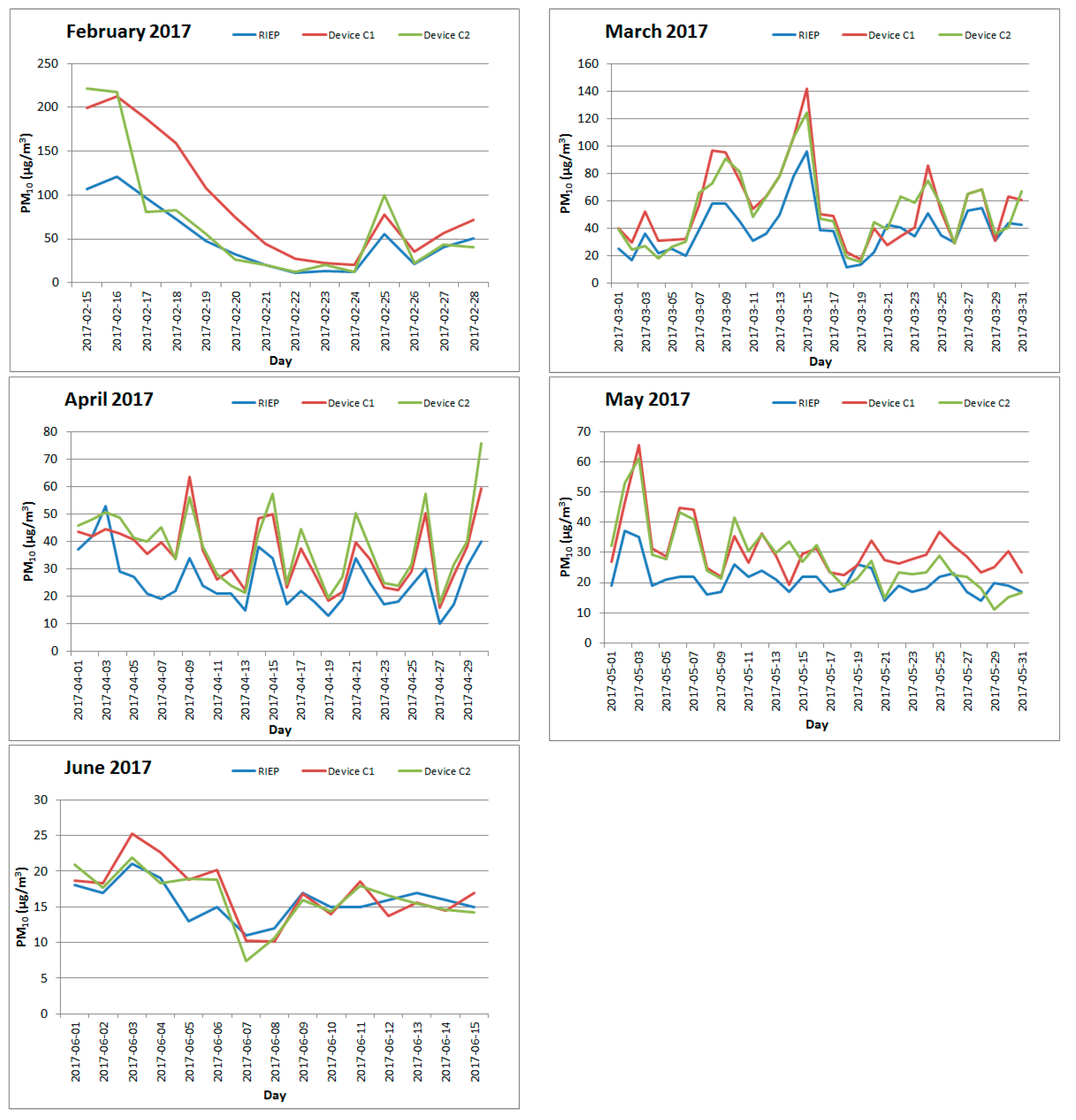
Mean absolute percentage error (%)	30.94	40.79	54.66	39.05	13.32	39.24

); that is the reason why the presented analysis was made for particular months (February–June 2017) separately. The graphical comparison of the raw measurements from the low-cost sensors and reference instrument (RIEP) can be found in Figure 2. The reference instrument measured only the PM₁₀ fraction; therefore, the analysis omitted the remaining fractions measured by the low-cost sensors.

Table 1 presents daily minimum, maximum, and average temperature and relative humidity in particular months, obtained from the RIEP station. The average daily temperature ranged from −2.5 °C (25 February 2017) to over +20 °C (30 May 2017), and the daily average relative humidity belonged to the range of 52% (2 June 2017) to 98% (25 May 2017). For the colder months (February, March, and April), it was usually closer to 80%, while for the warmer months (May and June), about 60%.

Table 2 and Table 3 show the values of some of the statistical parameters describing the raw PM₁₀ measurements made by both the low-cost devices, in particular months, and for the whole measurement period.

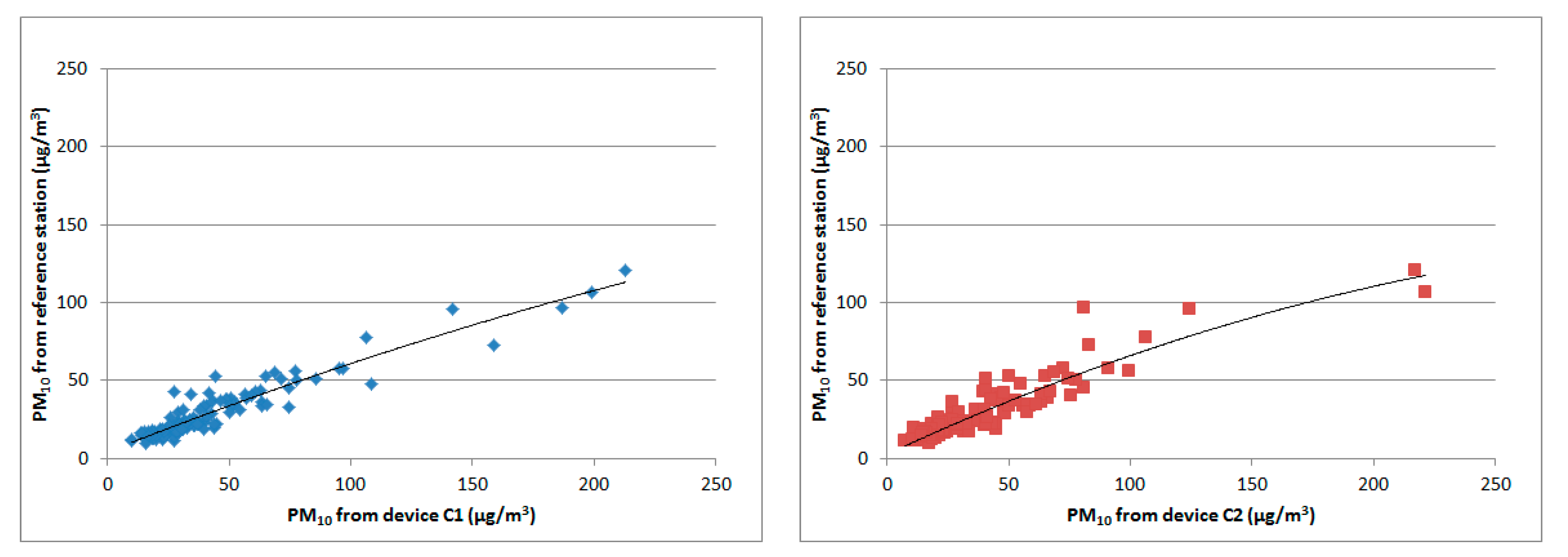
The collected results show a high correlation between the raw PM₁₀ measurements from the low-cost devices and measurements from the reference instrument. Pearson’s correlation coefficient ranges from r = 0.79 to r = 0.97 for device C1, while for device C2, from r = 0.77 to r = 0.91 (and is similar to results presented, e.g., in [13]). For both devices, this is a positive correlation. The highest r values were observed in months with the highest PM₁₀ concentrations, while for April, May, and June the correlation was slightly weaker. It is worth mentioning that, for the worst low-cost sensors, the determination coefficient R² was below 0.2. An example of such a case is the comparative measurements conducted within EuNetAir in Portugal [27]. Considering the values obtained in that study (R² from 0.13 to 0.36 for sensors Shinyei ppd42 and Shinyei PPD20V), the sensors used in Rabka-Zdrój were much better (in case of correlation). It should be remembered that climatic conditions were also much more diverse in Rabka-Zdrój than in Portugal.

In the vast majority of cases, the tested sensors overestimated the measuring values. The measured concentrations were usually 30–50% higher than these from the reference instrument. Device C2 was characterized by a little higher stability, for which the concentrations in February, March, and May were on average 34–36% higher than in the case of the reference instrument. In April, the average measurement results were higher by 50%. For device C1, the measured values were on average 38–48% higher than these from the reference instrument. Much higher values were obtained only in February—over 80%. It turns out that the reason for this much larger deviation, compared to the remaining months, are the days in the period 15–20 February, when the sensor indicated values twice higher than the reference instrument.

The tendency to overestimate the measured concentrations indicates also other statistical parameters; e.g., small differences between the absolute and relative errors. The mean error values were the highest for the beginning of the period. At the end of spring, both devices overstated the average measurements by no more than 10 μg/m³.

Figure 3 presents the relations between the measurement results (minimum, average, and maximum) from both the low-cost sensors and the reference instrument. The measurement range was divided into seven intervals, each of which covered 5 μg/m³. The minimum concentration of PM₁₀ in the analyzed measurement period was 10 μg/m³, while 44 μg/m³ was assumed as the upper limit since only individual values (24-h averages) were recorded above it. Figure 3 does not include values that exceed these levels, so as not to impair the readability of the illustrations.

For PM₁₀ concentrations in the range from 10 μg/m³ to 44 μg/m³, Figure 3 indicates a nearly linear dependence between measurements from both sensors and the reference instrument. A slight increase was noted in the low-cost sensors’ measurement overestimation at higher (over 30 μg/m³) PM₁₀ concentrations. In particular, for the analyzed intervals, the minimum values indicated by the low-cost sensors are very close to the average values measured by the reference instrument. The maximum values, in turn, significantly exceed the values from the reference instrument.

Considering the entire measurement period, both devices are characterized by high correlation coefficients. The measurement errors, in particular the absolute ones, are unfortunately also high, which is mainly due to the high concentrations observed during the cold period. The high value of the correlation coefficient and quite similar behavior of both sensors makes it possible to potentially use a correction function that will minimize the measurement errors. Determining the effective correction function is possible due to the fact that the training data set is quite extensive (242 daily averages), statistically significant, and includes various meteorological conditions (from winter to summer, in a temperate climate).

Practical observations pointed out that the percentage deviations between the measurement results from the low-cost sensors and the reference instrument were greater during higher PM concentrations. This hypothesis was confirmed by the results of the analysis, in which it turned out that, in the case of the tested sensors, the best fit (from linear, exponential, logarithmic, polynomial, and power correlation) gives a 2nd-degree polynomial correlation. The regression and correlation coefficients are presented in

Table 4. Regression curve for device C1 and C2 (February–June 2017, Rabka-Zdrój).

Month	Device C1	R2	Device C2	R2
February	0.000314x2 + 0.459x + 4.36	0.95	−0.00263x2 + 1.09x − 0.19	0.90
March	−0.000805x2 + 0.973x + 3.05	0.84	0.00342x2 + 0.253x + 15.2	0.85
April	−0.0107x2 + 1.48x − 11.8	0.66	−0.00681x2 + 1.14x − 7.08	0.64
May	0.001x2 + 0.519x + 5.95	0.61	0.00753x2 − 0.154x + 18.4	0.66
June	0.000732x2 + 0.454x + 7.89	0.59	−0.00252x2 + 0.594x + 6.85	0.56
Average	−0.000531x2 + 0.616x + 4.16	0.90	−0.000901x2 + 0.727x + 2.64	0.86

and Figure 4.

In an attempt to identify the factors affecting significant overestimation of the measurement results from the low-cost sensors, the relationship of the deviations in PM₁₀ concentrations measured by the low-cost sensors from the reference instrument was analyzed, taking into account the most important meteorological parameters.

Table 5. Pearson’s correlation coefficients between the deviations in PM₁₀ concentrations (24-h averages) from the low-cost sensors, in relation to the values from the reference instrument and meteorological parameters—device C1 (February–June 2017, Rabka-Zdrój).

Meteorological Parameter	February	March	April	May	June
Temperature	−0.26	−0.39	−0.21	−0.04	0.31
Relative humidity	0.65	0.28	0.58	0.55	0.33

and

Table 6. Pearson’s correlation coefficients between the deviations in PM₁₀ concentrations (24-h averages) from the low-cost sensors, in relation to the values from the reference instrument and meteorological parameters—device C2 (February–June 2017, Rabka-Zdrój).

Meteorological Parameter	February	March	April	May	June
Temperature	−0.31	−0.31	−0.34	−0.53	0.18
Relative humidity	0.35	0.67	0.63	0.47	0.35

present the Pearson’s correlation coefficients between the deviations in PM₁₀ concentrations and temperature, and the deviations in PM₁₀ concentrations and relative humidity in particular months of the measurement period. All of these correlation coefficients are statistically significant with p-values less than 0.01. The 24-h averages of the appropriate values were adopted for the calculations.

The results indicate that the degree of overestimation or underestimation of the PM₁₀ measurements is related to some meteorological parameters. This phenomenon is particularly strong in case of relative humidity. Figure 5 shows the deviations in the measurement values from the two low-cost sensors compared to the reference instrument, depending on the relative humidity.

It was a fairly moderate (from rather low to relatively high) positive correlation (r = 0.28–0.67), when comparing deviations in the measured PM₁₀ concentrations to the measurement results from the reference instrument with relative humidity. In general, the correlation coefficients were higher (up to r = 0.67) for colder months, where a high relative humidity (over 90%) occurred more often, and lower (r = 0.33–0.55) for warmer months, where the relative humidity was slightly lower (often below 60%). However, even then, for a high relative humidity, concentrations similar to the measurements results from the RIEP station occurred. 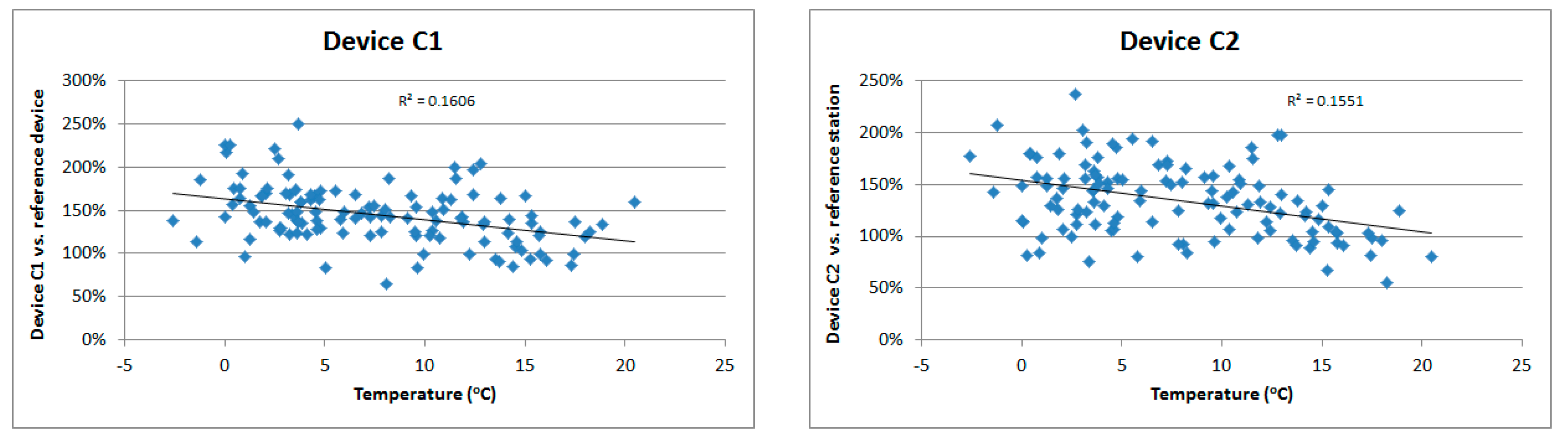This phenomenon may result from the fact that, in the case of high humidity, water droplets (for example from fog) floating in the air may be treated as aerosol particles [28]. In this situation, when absorbing air into the sensor, they cause (like solid particles) light scattering, so the device can treat them as pollutants. Days with high relative humidity in the Polish climate occur more often in the cold part of the year; therefore, this moves into a correlation between sensor readings deviations and temperature—this is presented in Figure 6. In this case, correlation coefficients are smaller, because low temperatures do not always have an impact on high humidity, and the temperature itself should not have a significant impact on the change in the deviations of the low-cost sensor measurements.

It can be pointed out that a high humidity and low temperature (often occurring together) may affect the overestimation of the optical sensors’ measurements (sometimes even more than twice). Conditions that favor underestimation include low humidity and high temperature.

The high correlation of the results means that with a large sample of data collected in various meteorological conditions, a fairly high consistency with the results from the reference instrument can be obtained with a correction function. A simple correction of the results may be based, for example, on the use of multiple regression, in which in the correction function of the measured PM₁₀ concentrations and the meteorological parameters with the greatest impact on the results—relative humidity—will be taken into account.

In order to determine the correction function, the analysis was carried out in two steps: First, with a 2nd-degree polynomial correlation, as the one for which the obtained agreement was the highest, the quadratic equation was determined, in which the average 24-h PM₁₀ concentrations from the low-cost sensors were treated as variables (Equation (1)). Next, the determined numerical values together with the results of the relative humidity measurements were applied in a multiple linear regression (Equation (2)) so that the final result depends on the corrected PM₁₀ concentration and relative humidity (Equation (3)).

P’ = −0.000712 × P² + 0.674 × P + 3.35

(1)

P_C = −0.187 × H + 1.007 × P’ + 14.2

(2)

P_C = −0.187 × H − 0.0007 × P² + 0.678 × P + 17.6

(3)

where:

P—measured PM₁₀ concentration by low-cost sensors (μg/m³);

H—measured relative humidity by low-cost devices (%);

P’—recalculated value of PM₁₀ concentration for low-cost sensors without relative humidity (μg/m³);

P_C—recalculated value of PM₁₀ concentration for low-cost sensors with relative humidity (μg/m³).

After recalculating the measurement results according to Equation (3), the statistical parameters for both devices take the values as shown in

Table 7. Basic statistical parameters of the measurements from device C1, after applying the correction function for the raw 24-h PM₁₀ concentration averages (February–June 2017, Rabka-Zdrój).

Parameter	February	March	April	May	June	Whole Period
Average PM10 concentration (μg/m3)	56.74	38.12	25.58	22.96	16.34	30.58
Average PM10 concentration (μg/m3)—RIEP	50.28	39.41	25.73	20.9	15.8	29.61
Ratio of average PM10 concentration: device C1/RIEP	1.12	0.97	0.99	1.1	1.03	1.03
Pearson’s correlation coefficient r; p < 0.01	0.98	0.92	0.84	0.81	0.82	0.95
Mean error (μg/m3)	6.46	−1.29	−0.15	2.06	0.54	0.97
Mean percentage error (%)	24.88	1.14	2.1	11.44	3.47	7.05
Mean absolute error (μg/m3)	7.96	5.18	3.06	2.84	1.66	3.94
Mean absolute percentage error (%)	26.99	15.31	10.18	14.2	10.69	14.53

and

Table 8. Basic statistical parameters of the measurements from device C2, after applying the correction function for the raw 24-h PM₁₀ concentration averages (February–June 2017, Rabka-Zdrój).

Parameter	February	March	April	May	June	Whole Period
Average PM10 concentration (μg/m3)	57.36	38.12	25.58	22.96	16.34	30.65
Average PM10 concentration (μg/m3)—RIEP	50.28	39.41	25.73	20.9	15.8	29.61
Ratio of average PM10 concentration: device C2/RIEP	1.14	0.97	0.99	1.09	1.03	1.03
Pearson’s correlation coefficient r; p < 0.01	0.98	0.92	0.84	0.81	0.82	0.94
Mean error (μg/m3)	7.07	−1.29	−0.15	2.06	0.54	1.04
Mean percentage error (%)	25.45	1.14	2.1	11.44	3.48	7.12
Mean absolute error (μg/m3)	8.57	5.18	3.06	2.84	1.66	4.01
Mean absolute percentage error (%)	27.56	15.31	10.18	14.2	10.69	14.6

.

After recalculating the measurement results using the correction function, the obtained results turn out to be much more similar to the results obtained in the measurements made with the reference instrument; this also resulted in a decrease of all errors. An important aspect is the size of the test sample. In the analyzed case, there were measurement results from the 4-month period, covering different seasons, starting from winter and ending almost at the beginning of summer.

Based on this training set, research is also being carried out to prove the equivalence (or conditions necessary to meet them) of measurements made using the low-cost PM sensors in relation to the reference methods. The results are presented in [23,29].

3.2. Verification of the Correction Function

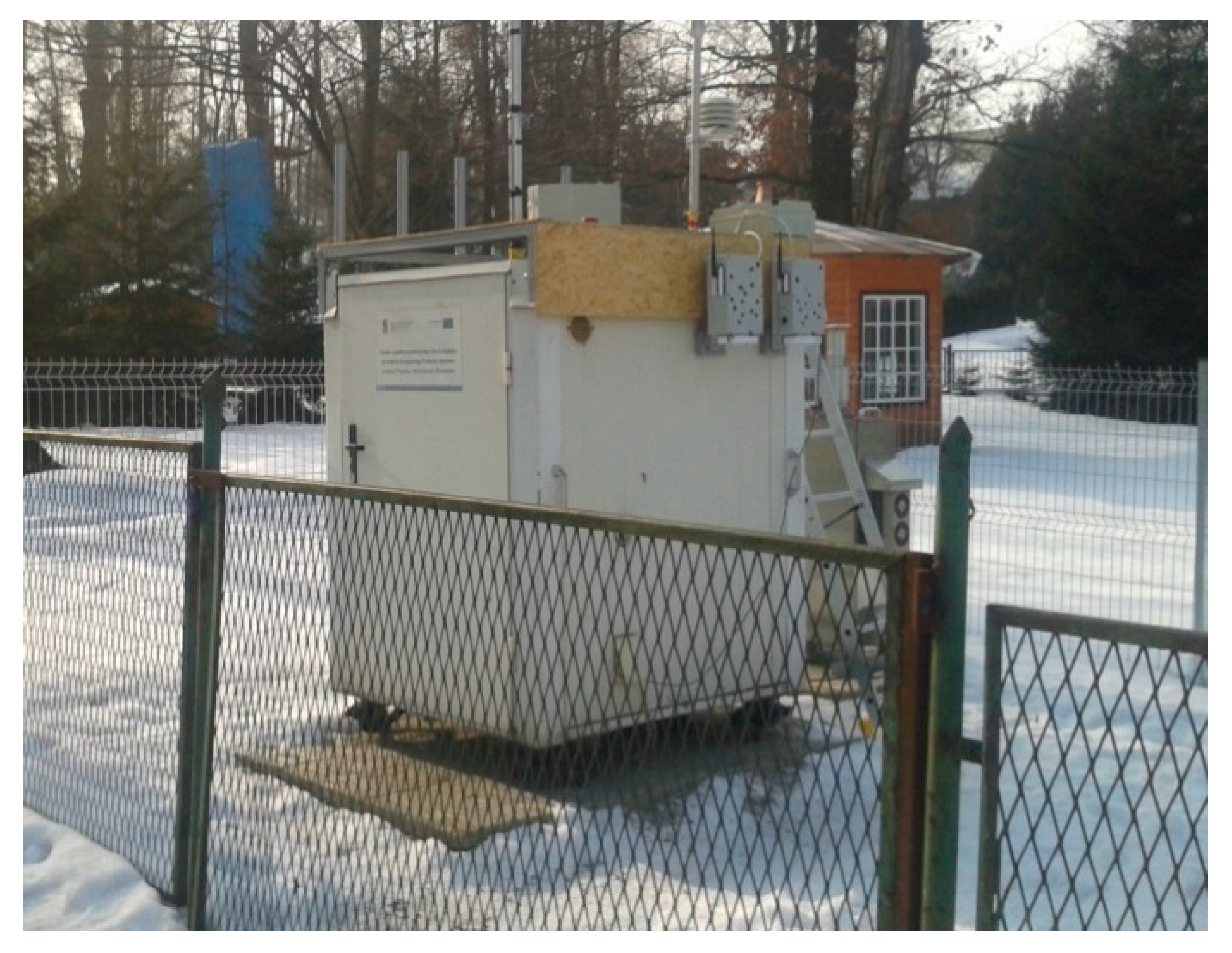
To verify the correction function, two identical devices with the new low-cost PM DFRobot sensors (named S1 and S2) were installed close enough to the reference air quality monitoring station (less than 10 m) in Nowy Sącz, in January 2018. It can be considered that these low-cost devices and the professional instrument operated in the same environment. The purpose of these devices was to verify the compliance of the measurement results with the concentrations observed by the reference instrument. The results from both the low-cost sensors were recalculated using the correction function determined on the basis of previous long-term measurements carried out in Rabka-Zdrój. The presented results include data from February to June 2018. Some statistical parameters are presented in

Table A1. Statistical parameters of the 24-h PM₁₀ concentrations—February 2018, Nowy Sącz.

Sensor	S1			S2
Correction	No	Without Humidity	With Humidity	No	Without Humidity	With Humidity
Pearson’s correlation coefficient	0.975	0.973	0.975	0.979	0.976	0.978
Maximum overvaluation compared to RIEP (μg/m3)	179.2	16.46	14.87	198.6	19.79	18.23
Maximum undervaluation compared to RIEP (μg/m3)	9.603	16.44	16.95	4.604	9.993	10.58
Mean error (μg/m3)	39.22	−3.65	−3.42	45.99	−0.04	−0.78
Mean percentage error (%)	47.26	−7.04	−8.21	59.19	−0.39	−1.5
Mean absolute error (μg/m3)	40.48	6.79	6.62	45.99	5.19	4.93
Mean absolute percentage error (%)	50.64	12.04	11.64	59.19	8.42	7.75

,

Table A2. Statistical parameters of the 24-h PM₁₀ concentrations—March 2018, Nowy Sącz.

Sensor	S1			S2
Correction	No	Without Humidity	With Humidity	No	Without Humidity	With Humidity
Pearson’s correlation coefficient	0.968	0.953	0.958	0.979	0.969	0.971
Maximum overvaluation compared to RIEP (μg/m3)	59.86	16.26	15.02	68.78	15.93	14.69
Maximum undervaluation compared to RIEP (μg/m3)	10.03	44.13	41.14	4.303	39.04	35.99
Mean error (μg/m3)	26.34	−8.9	−8.67	31.85	−6.24	−5.99
Mean percentage error (%)	36.83	−10.13	−11.06	44.91	−5.71	−6.6
Mean absolute error (μg/m3)	28.03	12.03	11.22	32.28	9.8	9.17
Mean absolute percentage error (%)	45.56	17.47	16.91	47.18	13.62	13.65

,

Table A3. Statistical parameters of the 24-h PM₁₀ concentrations—April 2018, Nowy Sącz.

Sensor	S1			S2
Correction	No	Without Humidity	With Humidity	No	Without Humidity	With Humidity
Pearson’s correlation coefficient	0.741	0.73	0.785	0.745	0.731	0.77
Maximum overvaluation compared to RIEP (μg/m3)	34.7	12.5	8.95	54.15	21.52	19.95
Maximum undervaluation compared to RIEP (μg/m3)	17.9	26.29	24.87	23.1	26.54	24.51
Mean error (μg/m3)	3.93	−6.8	−5.95	11.32	−2.14	−1.29
Mean percentage error (%)	13.44	−16.37	−14.2	33.66	−3.88	−1.67
Mean absolute error (μg/m3)	9.69	9.60	8.27	14.47	7.86	6.96
Mean absolute percentage error (%)	29.87	26.95	22.84	42.45	21.68	19.04

,

Table A4. Statistical parameters of the 24-h PM₁₀ concentrations—May 2018, Nowy Sącz.

Sensor	S1			S2
Correction	No	Without Humidity	With Humidity	No	Without Humidity	With Humidity
Pearson’s correlation coefficient	0.612	0.634	0.775	0.615	0.632	0.76
Maximum overvaluation compared to RIEP (μg/m3)	20.53	7.83	6.59	30.81	15.79	11.46
Maximum undervaluation compared to RIEP (μg/m3)	11.7	12.43	10.76	7.83	10.25	8.37
Mean error (μg/m3)	3.58	−2.52	−2.86	10.51	1.83	1.49
Mean percentage error (%)	17.34	−7.9	−10.3	48.25	11.57	9.41
Mean absolute error (μg/m3)	7.39	5.61	4.49	11.82	5.44	4.14
Mean absolute percentage error (%)	33.35	23.23	18.32	53.91	25.76	19.48

and

Table A5. Statistical parameters of the 24-h PM₁₀ concentrations—June 2018, Nowy Sącz.

Sensor	S1			S2
Correction	No	Without Humidity	With Humidity	No	Without Humidity	With Humidity
Pearson’s correlation coefficient	0.7	0.71	0.82	0.76	0.76	0.87
Maximum overvaluation compared to RIEP (μg/m3)	7.88	2.94	0.9	6.54	2.94	0.9
Maximum undervaluation compared to RIEP (μg/m3)	9.26	11.91	13.2	8.54	10.61	10.7
Mean error (μg/m3)	−0.69	−3.68	−5.68	−0.67	−3.67	−5.67
Mean percentage error (%)	−2.35	−15.8	−27.7	−2.83	−16.18	−28.0
Mean absolute error (μg/m3)	3.11	4.03	5.68	2.58	3.97	5.67
Mean absolute percentage error (%)	15.03	18.54	27.7	13.26	18.63	28.05

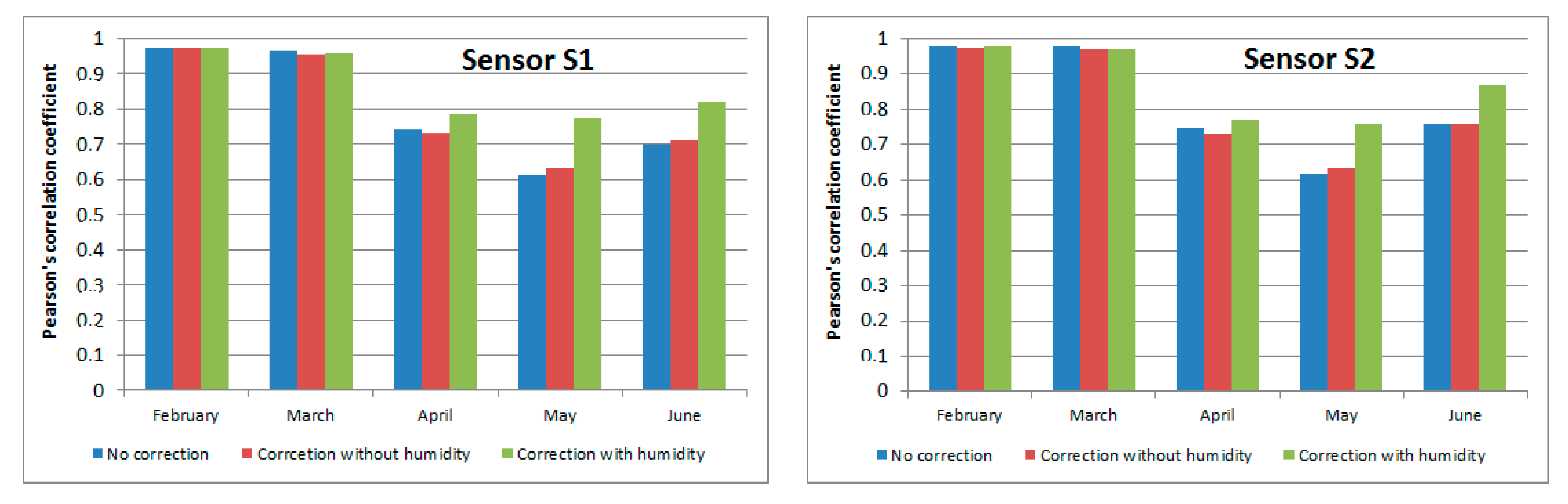
and in Figure 7, Figure 8, and Figure A1.

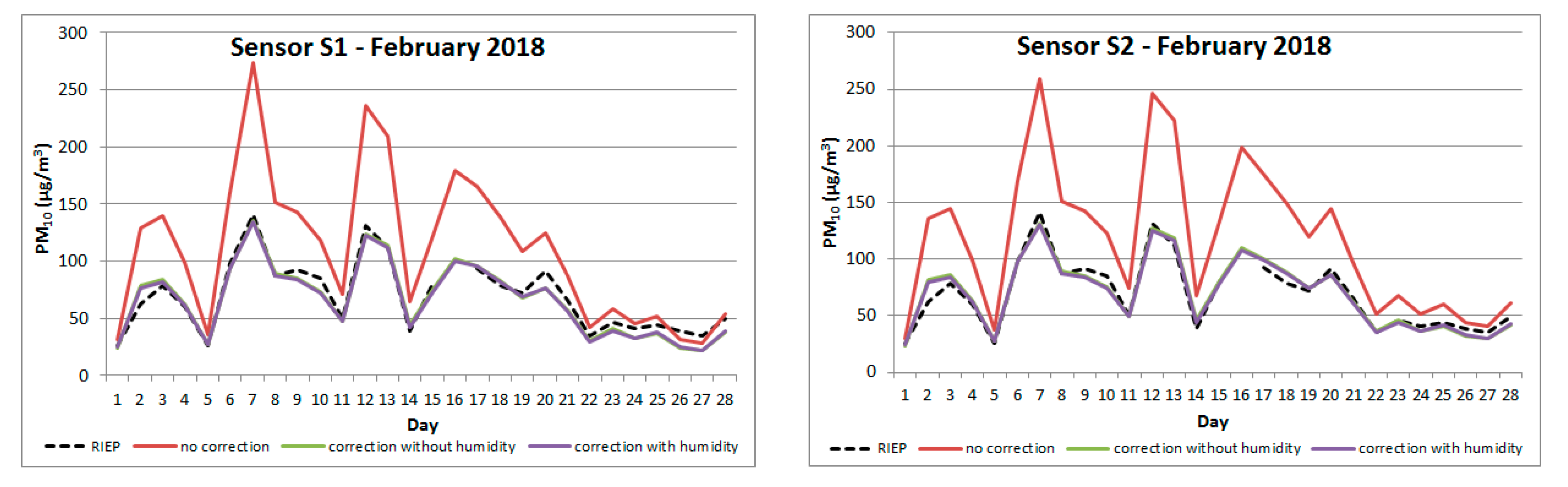
February 2018 was characterized by relatively low air temperatures, which contributed to the increase in PM₁₀ concentrations; this, in turn, also implied a significant over-estimation by both low-cost sensors. Values were higher by almost 50% in case of sensor S1 and almost 60% in case of sensor S2. The correlation coefficients for the two low-cost sensors and the RIEP station were very high—over 0.98. The largest differences between the concentrations measured in the reference station and the low-cost device were observed on 7 February. This day was characterized by one of the highest daily PM₁₀ concentration: 141 μg/m³.

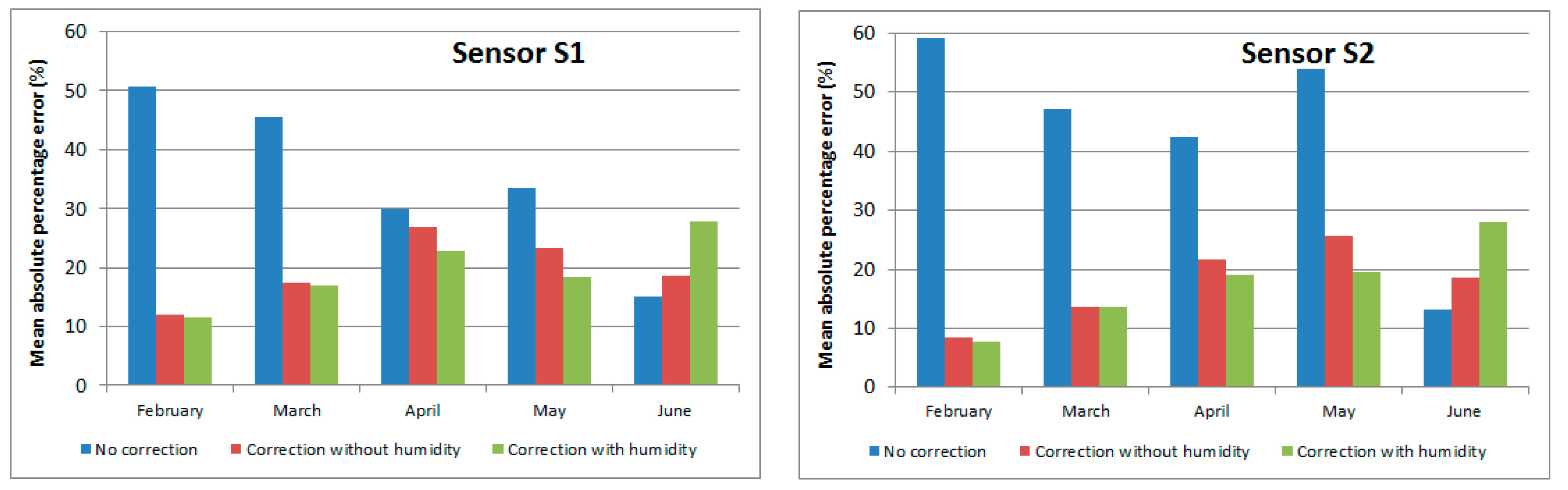
After applying the correction function, a significant improvement in the quality of PM₁₀ concentrations from both low-cost sensors was obtained. The correlation coefficients were still at a very high level, while the greatest improvement was observed in the case of percentage deviations and differences in absolute values (mean errors and percentage errors reached values below unity or slightly below zero). The average absolute percentage error was 9–12%, and deviations in relation to the concentrations measured at the reference station ranged from 17 μg/m³ to 20 μg/m³. There was also a significant reduction in concentration overdrafts in days with high PM₁₀ concentrations (7, 12, and 13 February), which is presented in Figure A1. The achievement of the desired effect of the correction function was undoubtedly due to the fact that it was determined on the basis of a comprehensive data set, taking into account a relatively long measurement period carried out under different atmospheric conditions.

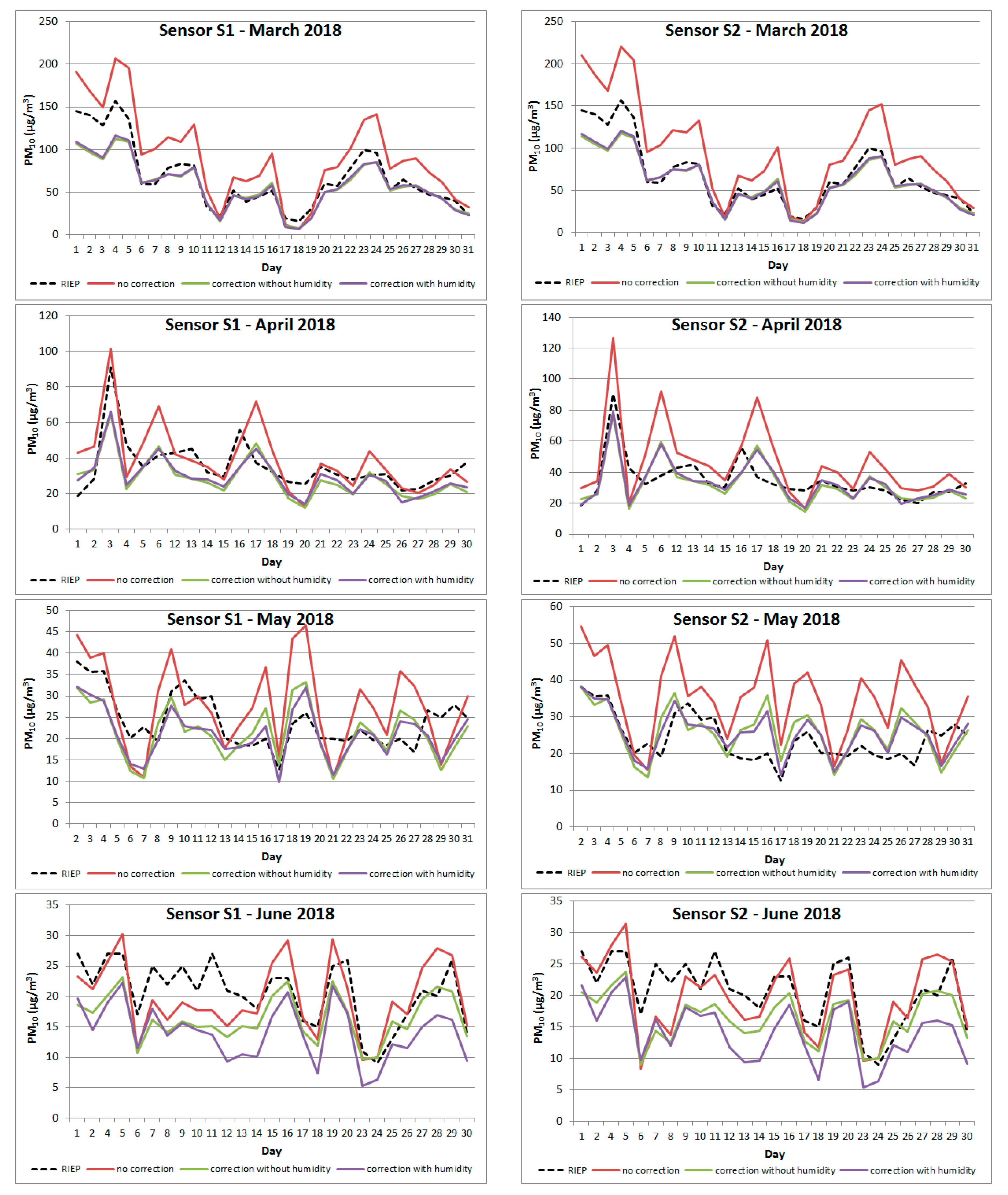
At the beginning of March, there were also very high concentrations (higher than in February), but in this case, the fit was not as good as in case of high concentrations in February. After applying the correction function, both sensors significantly underestimated the measured PM₁₀ concentrations. The situation returned to the regular one after 5 March. Thus, there appeared a question, how these days were different compared to others, in which high concentrations were also recorded. When analyzing the basic meteorological parameters (i.e., relative humidity, temperature, wind speed, and direction), one can observe that during the first days of March the temperatures were very low, reaching minima below −20 °C in the night and an average temperature below −15 °C (e.g., 1 March). In February, with the local maximum daily concentrations, the temperature usually fluctuated around zero (with indication of positive values). Then, the overestimation of the low-cost sensors even doubled. In case of the March maxima, the initial overestimation was only around 20–40% compared to the RIEP. The correction function reduced the values for the S1 and S2 sensors by almost half, which in case of the February, overshoots quite well the approximated adjusted value for the RIEP measurements, and for the exceedances of the first days of March; unfortunately, it caused a quite large undervaluation.

It seems that the reason for this was the humidity. As has been shown before, the optical sensors are affected by humidity, because small droplets of floating water, e.g., from fog, cause light scattering similar to PM particles. In case of high concentrations in February, there was a high relative humidity, and the temperature was close to 0 °C. At the beginning of March, the relative humidity was also quite high, but at a significantly lower temperature the actual number of water droplets in the same unit of air volume was significantly lower, compared to that with the same relative humidity but with the temperature almost 20 degrees higher (around 0 °C). A smaller number of water droplets probably resulted in less overestimation of the sensor. One can risk the hypothesis that the correction of the sensor readings should be based on absolute humidity. This would probably reduce the overestimation scale. Another potential solution would be to combine the corrective function with the temperature, or possibly including this parameter in a correction function below a certain temperature limit. The suitability of these approaches will be verified in further analysis.

In April and May, the correlation coefficients based on the raw measurements were slightly lower than in the two previous months. The application of the corrective function was therefore likely to bring an improvement, and this happened, especially in case of May, when a significant improvement in convergence resulted in the inclusion of meteorological conditions for both sensors. In these two months, the values of the measurement errors, in particular the absolute ones, significantly improved. In the end, their monthly value fluctuated around 20%, and the average errors below 6%.

In June, after applying the correction function, the values of the correlation coefficients also improved. The sensors, however, began to underestimate their values. The mean values of the absolute and percentage errors also increased. Perhaps the reason for this was the period on the basis of which the form of the corrective function was determined—cooler days with higher concentration values prevailed there—and also the fact that, in the warmer period, the PM concentrations in Poland are generally lower than in winter.

In most cases, applying the corrective function, from the initial tendency to overestimate the measurement values, led to underestimation. This is evidenced by the positive mean error for values without correction and then negative after applying the corrective function. The only exception was May for Sensor S2. In most cases, the error was at the level of a few μg/m³, especially for February, May, and partially April. The worst case was in March, when the error values were close to 10 μg/m³. This regularity is also visible when comparing the maximum daily deviations above and below the values from the reference measurement devices. For the raw data, it is possible to shift this range towards significant revaluations, and after applying the correction, the center of this range moves towards zero or in a few cases it takes a negative value.

It is also worth paying attention to the issue of the error, depending on taking into account the relative humidity in the correction function. For a definite improvement in the accuracy of the results, it is enough to use the correction function without taking into account the variability of humidity, thanks to which it is possible to improve the results by several dozen percent. The use of the extended form of the correction function slightly improves some of the indicators, but the added improvement is not so significant.

Using the correction functions in the analyzed cases resulted in a significant improvement and led to getting acceptable quality levels of the source measurement results. Taking into account additional meteorological parameters (such as relative humidity, and perhaps wind speed, which will be the subject of further analysis) may bring even better improvement in the measurement results of low-cost devices in relation to results from reference stations.

4. Conclusions

The results of the measurements and their subsequent analysis presented in the article prove that the quality of the analyzed low-cost PM sensors depends on the season. In the case of the winter months (February, March), they were characterized by a high correlation with the reference device (r > 0.97); however, the measurements were characterized by a high long-term mean absolute percentage error, even over 50%. They tend to have overestimated results (similar to the low-cost sensors of other manufacturers). In the case of spring and summer months, the measurements were characterized by a much lower correlation value (r < 0.7), but also a slightly lower value of the long-term mean absolute percentage error (<30% in June).

After applying the proposed correction function, the obtained results are much closer to the concentration measured using the reference air quality monitoring methods. For the winter months, the values of the correlation coefficients remained at the same high level, but it was possible to significantly reduce the error values, in particular the mean absolute percentage error (up to 7–17%). In the case of warmer months, the value of the correlation coefficient significantly improved (up to r = 0.87). Therefore, it seems that the corrective function fulfills its role, especially in the winter months, when the PM₁₀ concentrations are the highest in Poland.

The use of measuring devices, based on low-cost PM sensors, can be an effective supplement to the conventional monitoring network, enabling the achievement of a higher spatial resolution of measurements, without incurring significant financial outlays. The condition for the use of such devices is the need to properly care for their quality, servicing, ongoing monitoring, periodic calibration with reference devices, etc. It should also be remembered that such devices are characterized by a much higher measurement uncertainty compared to the reference ones; therefore, they can only be a supplement and not an alternative to professional instruments. Further analysis is planned to be conducted, including the use of a much longer measurement series and taking into account other parameters in the correction functions that may affect the deviations in the low-cost measurements compared to the reference methods.