Article

The Microscale Urban Surface Energy (MUSE) Model for Real Urban Application

Department of Atmospheric Science, Kongju National University, Gongju 32588, Korea
*
Author to whom correspondence should be addressed.
Atmosphere 2020, 11(12), 1347; https://doi.org/10.3390/atmos11121347
Submission received: 11 November 2020 / Revised: 1 December 2020 / Accepted: 9 December 2020 / Published: 12 December 2020
(This article belongs to the Section Atmospheric Techniques, Instruments, and Modeling)

Abstract

:
Urban atmospheric environmental issues are commonly associated with the physical processes of urban surfaces. Much progress has been made on the building-resolving microscale atmospheric models, but a realistic representation of the physical processes of urban surfaces on those models is still lacking. This study presents a new microscale urban surface energy (MUSE) model for real urban meteorological and environmental applications that is capable of representing the urban radiative, convective, and conductive energy transfer processes along with their interactions, and that is directly compatible with the Cartesian grid microscale atmospheric models. The physical processes of shadow casting and radiative transfers were validated on an analytical accuracy level. The full capability of the model in simulating the three-dimensional surface heterogeneities in a real urban environment was tested for a hot summer day in August 2016 using the field measurements obtained from the Kongju National University campus, South Korea. The validation against the measurements showed that the model is capable of predicting surface temperatures and energy balance fluxes in a patch scale at the heterogeneous urban surfaces by virtue of the interactive representation of the urban physical processes. The excellent performance and flexible grid design emphasize the potential capabilities of the MUSE model for use in urban meteorological and environmental applications through the building-resolving microscale atmospheric models, such as computational fluid dynamics (CFD) and large-eddy simulations (LES).

1. Introduction

Microscale atmospheric models, such as computational fluid dynamics (CFD) and large-eddy simulations (LES), have been widely used to simulate urban flow, turbulence, and pollutant dispersion in urban environments (e.g., [1,2,3,4,5,6]). Many previous studies focused on understanding urban flow behaviors and associated dispersion characteristics using extremely simplified urban geometries. For example, Kim and Baik [7] investigated the flow and dispersion characteristics in a single canyon by changing the canyon aspect ratio (that is, the ratio of building height to canyon width). Lin et al. [8] and Ramponi et al. [9] examined the influence of street width on local ventilation, and Hang et al. [10] demonstrated a significant impact of building height change on ground-level pollutant concentrations using simple cubic array type geometries.
Recently, the models’ applications have rapidly extended to answer urban atmospheric environmental issues of real urban environments such as ventilation for wind and thermal comfort (e.g., [11,12,13,14,15]). The change is attributed to urban geographical information data and computing resources [16]. The geographic information system (GIS) data that characterize the morphological features of urban surfaces in many cities for buildings, streets, trees, and others have been readily available (e.g., [17]). Moreover, the development of high-performance computers has made CFD and LES models available for real urban surface simulations (e.g., [18,19,20]). Letzel et al. [19] investigated microscale ventilation of an urban district in Hong Kong using the PArallelized Large-eddy simulation Model (PALM). Park et al. [20] examined turbulence characteristics in a densely built-up urban area (Seoul) in South Korea using the PALM. Meanwhile, Kanda et al. [21] conducted hundreds of LES simulations for building blocks (Tokyo and Nagoya) in Japan in order to develop an urban surface drag parameterization. Nakayama et al. [22] applied an LES model to simulate plume dispersion characteristics for urban districts (Tokyo) in Japan for use in emergency response.
Despite the extension of the models’ applicability, there are still significant problems in the use of the microscale atmospheric models [23]. Intensive computing time is one of the critical barriers to real urban applications. As an effort to handle the problem, Gowardhan et al. [24] developed a CFD-based wind solver for fast calculation of urban flows without oversimplifying urban dynamical processes. Generally, the models are developed using parallel programmings, such as a message passing interface (MPI), in order to use multiple computer processors. The accurate representation of urban physical processes is another critical issue for microscale real urban simulations. Many studies have emphasized the importance of thermal heterogeneities in the atmosphere and urban surfaces on urban flow and dispersion from idealized urban simulations (e.g., [25,26,27,28,29,30,31,32,33,34,35]). For example, Yang and Li [29] showed that the in-canyon flow depends strongly on thermal stratification in case of weak winds. Nazarian and Kleissl [32] examined the changes of in-canyon vortex flow in terms of strength and location according to the surface heating of idealized canyon surfaces. Wang and Ng [35] investigated the influence of the surface thermal forcing on pedestrian-level wind speeds in a real urban district in Hong Kong. However, there is a limitation that the homogeneous surface heating was assumed with a specific value over the whole urban area. The thermal heterogeneities of urban surfaces may change significantly according to building morphology and weather conditions.
The thermal heterogeneities of urban surfaces have often been revealed from remote sensing and in situ measurements at different spatial scales (e.g., [36,37,38,39]). Urban surface models have also been developed to investigate the influence of the small scale variation of the urban surface heterogeneities (e.g., [40,41,42,43]). Krayenhoff and Voogt [40] developed the Temperatures of Urban Facets in 3-D (TUF-3D) model to investigate microscale thermal anisotropy. Yaghoobian and Kleissl [41] implemented an indoor–outdoor building energy simulator (IOBES) into the TUF-3D model to study urban effects on building energy use. These urban surface models have been used in microscale atmospheric models in investigating the surface thermal effects on urban flow and dispersion for idealized canyon geometries [31,44,45]. Meanwhile, Yang and Li [42] developed the Model for Urban Surface Temperature (MUST) for arbitrarily configured building clusters [46], and Resler et al. [47] implemented an urban surface model (USM) into the PALM that parameterizes various urban physical processes. The more recent models showed potential capabilities of simulating surface heterogeneities for complicated urban geometries.
Accurate representation of the urban physical processes is a prerequisite for the reproduction of realistic thermal heterogeneities of urban surfaces, which is essential in microscale meteorological and environmental simulations of urban flow and dispersion in real urban environments. However, realistic reproduction of the urban thermal heterogeneities detected in real urban environments still lacks (e.g., [41,42]), and the model’s compatibility with microscale atmospheric models is not tested thoroughly for real urban environments (e.g., [40,41,46]). This study aims to present a new microscale urban surface energy (MUSE) model for real urban meteorological and environmental application that is capable of representing the essential urban physical processes and their interactions, and that is compatible directly with the Cartesian grid microscale atmospheric models. The MUSE model’s structure is compared to the well-known previous TUF-3D model in Appendix A. The remainder of this paper is structured as follows. Section 2 describes details of the MUSE model, including grid representation of urban geometries and associated physical parameterizations of shortwave and longwave radiative transfers, turbulent heat exchanges, and conductive heat transfer on urban surfaces. Section 3 describes field measurements and model configuration used for validation of the full capability of the MUSE model, and Section 4 presents the validation results of the urban physical processes and comparisons against the field measurements. A summary and conclusions follow in Section 5.

2. Description of the Microscale Urban Surface Energy (MUSE) Model

2.1. Grid Representation and Urban Physical Processes

2.1.1. Grid Representation of Urban Surfaces

Real urban surfaces consist of various artificial and natural obstacles such as buildings, roads, trees, and grasses, and their different combinations create unique urban geometries. The realistic representation of the urban surfaces is a prerequisite in parameterizing urban physical processes for microscale flow and dispersion simulations. The MUSE model represents the urban surfaces with three-dimensional structures of grid cells on a Cartesian grid system (Figure 1a). Each grid cell has six “patches” of two horizontal (top and bottom) surfaces and four vertical (east, west, south, and north) wall surfaces. Among them, the patches facing the atmosphere are defined as active patches, on which surface energy exchange processes are calculated between the patch and the corresponding atmospheric model grid.
The MUSE model is designed to the three-dimensional grid structure that is compatible directly with general microscale atmospheric models (Figure 1b). Thus, the interaction between microscale atmospheric models and the MUSE model can be calculated efficiently with both “online” or “offline” modes. Table 1 lists the meteorological forcing variables and the predicted variables of the MUSE model. The online computation means that the time integration of the MUSE model and any microscale atmospheric model can be undertaken in a simultaneous step with each other. In other words, the MUSE model predicts the surface energy balance fluxes and surface temperatures at each patch given meteorological fields by the microscale atmospheric model, and the microscale atmospheric model predicts three-dimensional meteorological fields using the surface energy balance fluxes or surface temperatures as a bottom boundary condition. In offline computation mode, the predictions of the MUSE model and the microscale atmospheric model are conducted sequentially no matter which model runs first. When meteorological forcing measurements are available, it is recommended to use the offline mode computation in reproducing the thermal heterogeneities of the entire urban area. Generally, current microscale atmospheric models cannot provide radiative and thermal forcing of the MUSE model as accurate as measurements due to lack of corresponding physical representation. When it comes to dynamic forcing (that is, wind fields), measurements have limitations in representing spatial heterogeneities of complicated urban surfaces due to low instrumentation density. The neutral simulation of microscale atmospheric models might be a better choice because of the models’ capability in resolving surface drags of buildings. Overall, the colocated grid design makes the MUSE model flexible to meteorological forcing in any combination with microscale atmospheric models and measurements.

2.1.2. Urban Physical Processes

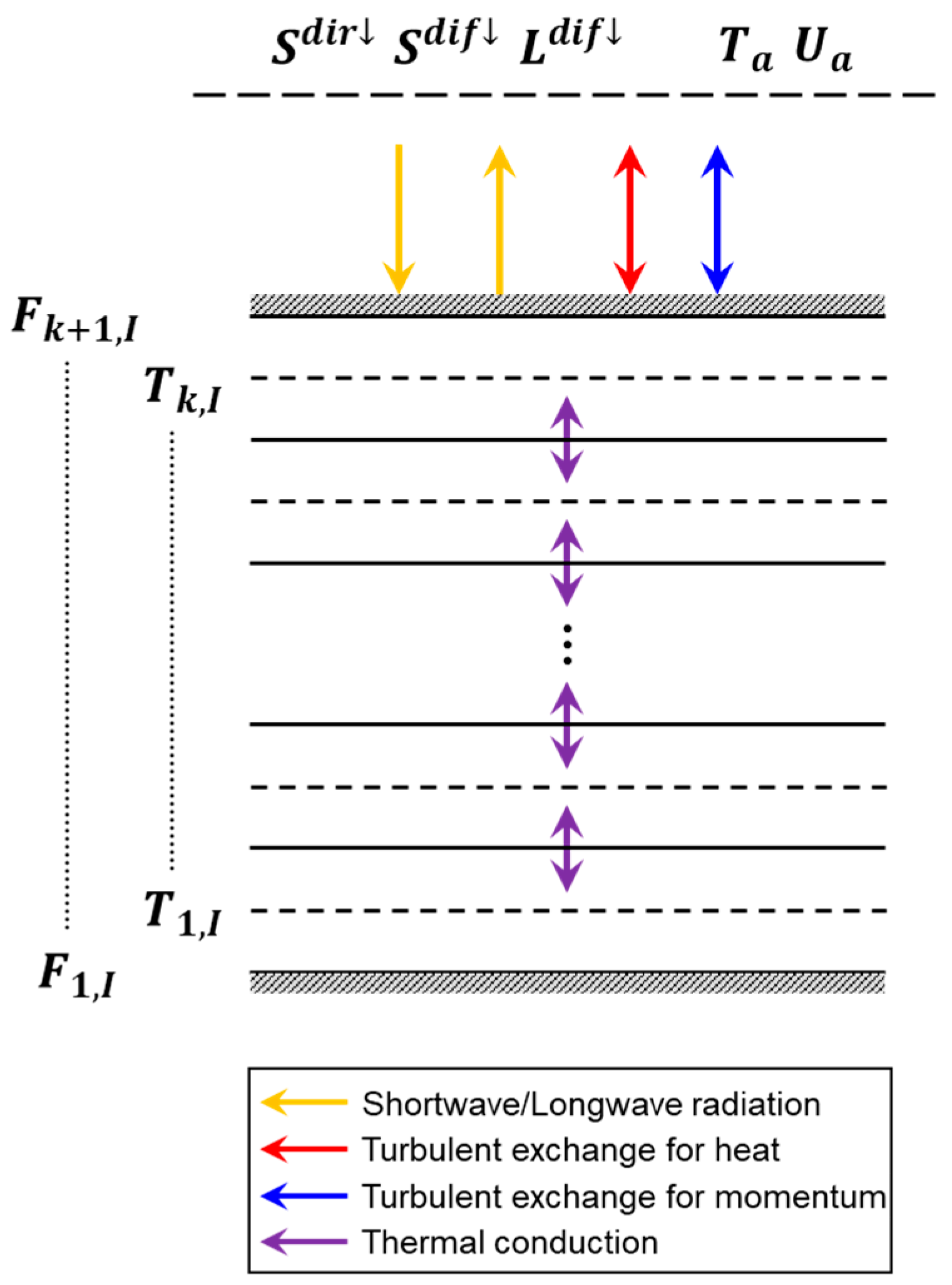
Various physical processes associated with the complicated urban surfaces interact, resulting in the formation of unique urban microclimates (e.g., [48,49,50,51,52,53,54,55,56]). The MUSE model includes the urban physical processes that are shortwave and longwave radiative transfers within the canyon, turbulent sensible heat exchanges at each patch surface, and conductive heat transfer within multiple interior subsurface layers over an urban area (Figure 2). It also includes a shadow submodel and the formulations of three-dimensional patch–patch view factor estimation for the radiative transfer parameterization. All of those physical processes interact simultaneously among them during the model integration, leading to realistic reproduction of the urban surface heterogeneities in surface energy balance fluxes and surface temperature.
The urban surfaces of buildings and roads are made with diverse construction materials such as concrete, brick, and asphalt. Thus, the urban surface simulation needs to characterize the urban surfaces realistically in association with urban physical processes. The MUSE model characterizes urban surfaces using the physical property parameters assigned at each patch of the simulation domain. Table 2 lists the physical property parameters of the MUSE model used to represent the physical properties of urban surfaces. The surface roughness lengths for momentum and heat are the aerodynamic property parameters associated with turbulent momentum and heat exchanges, respectively. The surface albedo and emissivity are the radiative property parameters of urban surfaces, and the thermal conductivity and volumetric heat capacity are the thermal property parameters of the interior subsurfaces. Each patch has all the physical property parameters assigned according to urban surface materials.

2.2. Radiation Processes

2.2.1. Shadow Model

A shadow model is developed as an ingredient of the MUSE model based on a geometric ray casting approach. In real urban environments, the shadow geometry of each building depends on the relative position of the surrounding buildings and the sun. The shadow model at first step computes the shadow lengths at each rooftop patch of buildings cast on horizontal and vertical surfaces, and then it determines the sunlit/shaded condition at every patch (Figure 3). The shadow length by the patch I of a building rooftop cast on a horizontal surface ( l h o r , I ) can be analytically determined by
l h o r , I = h I tan θ z ,
where h I is the height of the patch I of a building rooftop and θ z is the solar zenith angle. The vertical shadow length at a certain point is computed along the horizontal shadow path ( l v e r t , I ) by
l v e r t , I = ( l h o r , I l P , I ) tan ( π 2 θ z ) ,
where l P , I ( = Δ x 2 + Δ y 2 ) is the horizontal distance between the point and the patch I . Here, the point location is defined by a relative distance separated from the patch I with Δ x and Δ y . Therefore, the shaded patches by the patch I of a building are determined as the patches that exist on the horizontal and vertical shadow paths. The MUSE model inspects every patch on the horizontal shadow path moving forward from the location of patch I with a small distance step of ( d x , d y ) = ( L cos θ a , L sin θ a ). Here, θ a is the solar azimuth angle and L is the step size of length.
The solar zenith angle ( θ z ) and solar azimuth angle ( θ a ) at the center of model domain are calculated by
cos θ z = sin ϕ sin δ + cos ϕ cos δ cos ω t ,
cos θ a = cos θ z sin ϕ sin δ sin θ z cos ϕ ,
where ϕ is the latitude of the model domain, δ is the solar declination angle, and ω t is the solar hour angle. The value of θ a is set to increase clockwise from the due north.

2.2.2. Patch View Factors

The three-dimensional view factors are necessary for calculating radiative energy exchange processes within urban canyons. Each patch sees other patches and/or the sky. When considered for two patches I and J , the patch–patch view factor ( ψ I J ) denotes the fraction of the radiation reached at the patch I to that emitted from the patch J [57]. Similarly, the patch–sky view factor ( ψ I s k y ) at the patch I indicates the fraction of radiation reached from the sky. Generally, analytical methods can be used for calculating ψ I J in simple urban geometries (e.g., [58,59,60]). However, they do not apply to complicated morphologies in real urban environments. Some previous studies have used ray tracing algorithms (e.g., [40,42,43]). When a large number of photons tracks in the algorithm, it can calculate the view factors with high computation accuracy [61,62]. However, it inherently requires tremendous computing time to compute the view factors over hundreds of buildings for real urban simulations. Lee et al. [63] suggested a new numerical computation method for patch–patch view factor calculation to solve the limitation. The method was derived from the analytical view factor formulation, which can be applied to arbitrarily facing patches and is not limited to any specific patch orientation.
In this study, the analytically-based numerical method by Lee et al. [63] is used for perpendicular and parallel patches to calculate the patch–patch view factors and the patch–sky view factors (Figure 4). When the two patches I and J are perpendicular to each other with a distance of R , the patch–patch view factor ( ψ I J ) can be computed as follows:
ψ I J E W = Δ X Δ Z π R 4 Δ A J ,   ( for east/west walls )
ψ I J S N = Δ Y Δ Z π R 4 Δ A J ,   ( for north/south walls )
where ψ I J E W and ψ I J S N are the patch–patch view factors from the horizontal patch I to the vertical patch J on east/west and north/south walls, respectively. Δ X = | x I x J | , Δ Y = | y I y J | , and Δ Z = | z I z J | are the directional distance between the two patches ( R = Δ X 2 + Δ Y 2 + Δ Z 2 ). Δ A J is the area of patch J ( Δ A J = Δ y J Δ z J for the east or west wall, Δ A J = Δ x J Δ z J for the north and south wall, Δ A J = Δ x J Δ y J for horizontal surface). When the two patches I and J are parallel to each other with a distance of R , the patch–patch view factor ( ψ I J ) can be computed as follows:
ψ I J E / / W = Δ Y 2 π R 4 Δ A J ,   ( for east/west walls )
ψ I J S / / N = Δ X 2 π R 4 Δ A J ,   ( for north/south walls )
where ψ I J E / W and ψ I J S N are the patch–patch view factors from the vertical patch I to the vertical patch J on east/west and north/south walls, respectively. From simple algebra relation of view factor, the patch–sky view factor ( ψ I s k y ) at a horizontal or vertical patch can be calculated as follows:
ψ I s k y = 1 J = 1 N ψ I J ,   ( for horizontal patch   I )
ψ I s k y = 0.5 J = 1 N ψ I J ,   ( for vertical patch   I )
where N denotes the number of patches that are facing the patch I . Note that N is determined for vertical patches by the patches that are above a horizontal plane from the patch I .

2.2.3. Shortwave Radiation

The shortwave radiative fluxes reaching every patch are composed of the direct and diffuse shortwave radiation. The direct shortwave radiative flux at the patch I ( S I d i r ) is calculated by
S I d i r = S d i r cos c I cos θ z f s u n l i t ,
where S d i r is the direct shortwave radiation at the horizontal surface from the sky, and c I is the solar incidence angle on the patch I , and f s u n l i t is the surface sunlit fraction. f s u n l i t is determined by the shadow model as a value of 1 (sunlit) or 0 (shaded) at each patch. The solar incidence angle on the patch I ( c I ) is calculated as
cos c I = cos β I cos θ z + sin β I sin θ z cos ( θ a γ I ) ,
where β I and γ I are the slope angle and azimuth angle of the patch I , respectively. The value of γ is set to increase clockwise from the due north as θ a . This equation can apply for arbitrarily tilted surfaces. In the MUSE model, β has 0 for horizontal (roofs and roads) patches or π 2 for vertical (walls) patches. Thus, the resultant S I d i r is identical to the downward shortwave radiation from the sky ( S d i r ) for horizontal sunlit patches and that is S d i r cos c I cos θ z for vertical sunlit patches. It is assigned to 0 W m−2 for the other shaded patches. On the other hand, the diffuse shortwave radiative flux at the patch I ( S I d i f ) can be calculated by
S I d i f = S d i f ψ I s k y ,
under the assumption that the downward shortwave radiation from the sky ( S d i f ) is isotropic.
The reflected shortwave radiative flux reaching the patch I from the other patch J can be expressed as
S I , m + 1 R = α I ( J = 1 N ψ I J S J , m R ) ,
where S I , m + 1 R is the reflected shortwave radiative flux by the patch I reaching from the other patches J at ( m + 1 )th reflection, α I is the surface albedo of the patch I , N is the number of the patches J interacting with the patch I , and S J , m R is the shortwave radiative flux reflected from the patch J after m th reflection. Here, the Lambertian reflection is assumed at every surface. The initial reflected shortwave radiative flux at each patch can be calculated by S I , 1 R = α I ( S I d i r + S I d i f ) . The resultant net shortwave radiative flux absorbed at the patch I ( S I * ) can be expressed as
S I * = ( 1 α I ) ( S I d i r + S I d i f + m = 1 M S I , m R ) ,
where M is the number of reflection considered for radiative energy trapping within urban canyons, and three times reflection applies to the computation of shortwave radiation in the MUSE model.
Meanwhile, the reflection computation is a time- and memory-consuming process. The MUSE model applies the compressed row storage scheme suggested by Yang and Li [42]. The number of patches interacting with the patch I limits with a small fraction of the entire patches, meaning that most of ψ I J is zero. The compressed row storage scheme takes only nonzero values into account, which results in a significant reduction of computational cost for calculating multiple reflection. Because the scheme is simply to rearrange the nonzero view factor patches for computational efficiency, it causes no additional computational error. The MUSE model assumed a minimum threshold value of 1.2 × 10⁻²⁰ to further enhance computational efficiency, which leads to a negligible difference in surface temperature.

2.2.4. Longwave Radiation

Unlike shortwave radiation, the MUSE model considers the longwave radiation emitted from the whole patches as well as the downward longwave radiation from the sky. The diffuse longwave radiative flux reaching the patch I ( L I d i f ) is calculated by
L I d i f = L d i f ψ I s k y ,
where L d i f is the downward longwave radiative flux from the sky. The longwave radiation emitted from the patch I ( L I ) is calculated following the Stefan–Boltzmann equation as follows:
L I = ε I σ T I 4 ,
where ε I and T I are the surface emissivity and surface temperature of the patch I , respectively, and σ is the Stefan–Boltzmann constant (=5.67 × 10⁻⁸ W m−2 K−4).
The computation of the reflection process of longwave radiation is similar in shortwave radiation except that the longwave radiation emitted at each patch is considered along with the diffuse longwave radiation from the sky. The reflected longwave radiative flux reaching the patch I from the other patch J can be expressed as
L I , m + 1 R = ( 1 ε I ) ( J = 1 N ψ I J L J , m R ) ,
where L I , m + 1 R is the reflected longwave radiative flux from the patch I reaching from the other patches J at reflection ( m + 1 )th reflection, ε I is the surface emissivity of the patch I , N is the number of patches J , and L J , m R is the longwave radiative flux reflected from the patch J after ( m )th reflection. The initial reflected longwave radiative flux at each patch can be calculated by L I , 1 R = ( 1 ε I ) ( L I d i f + L I ) . The resultant net longwave radiative flux absorbed at the patch I ( L I * ) can be expressed as
L I * = ε I ( L I d i f + m = 1 M L I , m R L I ) ,
where M is the number of reflection considered for radiative energy trapping within urban canyons, and one reflection applies to the computation of longwave radiation in the MUSE model.

2.3. Turbulent Sensible Heat Exchange

2.3.1. Horizontal Roof and Road Patches

The MUSE model applies the Monin–Obukhov similarity relation for calculating turbulent sensible heat fluxes at the horizontal roof and road patches. Even though it is difficult to justify the applicability of Monin–Obukhov similarity relation on a theoretical basis, many mesoscale and microscale modeling studies apply the formulation with a practical purpose to determine physical fluxes at urban surfaces (e.g., [64,65]). The turbulent sensible heat flux at the horizontal patch I ( H I ) is given following Lee and Park [64] by
H I = ρ c p u * T * = ρ c p κ 2 F h ( z I z 0 , I ,   z I z 0 T , I ,   R i B ) U a ( T a T I ) ln z I z 0 , I ln z I z T , I ,
where ρ is the air density (kg m−3), c p is the specific heat capacity at constant pressure (J kg−1 K−1), u * is the friction velocity (m s−1), and T * is the temperature scale (K). κ is the von Kármán constant, z 0 , I and z 0 T , I are the surface roughness lengths for momentum and heat, respectively, R i B is the bulk Richardson number ( = g z Δ T θ ¯ U a 2 ), and Fh is the atmospheric stability correction function. T I is the surface temperature of the patch I , and T a and U a are the temperature and wind speed at the adjacent atmospheric grid of the patch I , respectively.

2.3.2. Vertical Wall Patches

The empirical formulation based on Rowley et al. [66] has been widely applied for calculating the convective heat flux at vertical surfaces (e.g., [40,67]) because the use of the Monin–Obukhov similarity relation for vertical surface fluxes calculation is arguable. In the MUSE model, the turbulent sensible heat flux at the vertical patch I ( H I ) is given by
H I = h c ( T I T a ) ,
where T I is the surface temperature of the vertical patch I , and T a is the air temperature at the adjacent atmospheric grid cell of the patch I . The convective heat transfer coefficient ( h c ) is given by
h c = 11.8 + 4.2 U a ,
where U a ( = U 2 + V 2 + W 2 ) is the wind speed at the adjacent atmospheric grid cell of the patch I . The empirical formulation was obtained from in situ measurements [66].

2.4. Subsurface Heat Conduction

Every active patch consists of multiple subsurface layers to represent conductive heat transfers in buildings and grounds. This process is one of the essential physical processes in the formation of urban heat islands [68]. The MUSE model assumes that the conductive heat process occurs in a one-dimensional column (Figure 2). From the conservation of energy, the media temperature at each subsurface layer of the patch I can be calculated with an explicit finite differencing by
T k , I n + 1 = T k , I n Δ t C k , I Δ z k ( F k + 1 , I n F k , I n ) ,
where T k , I n is the media temperature of the subsurface layer k of the patch I at n th time step, C k , I is the volumetric heat capacity of the subsurface material, Δ z k is the depth of each sublayer, and Δ t is the integration time interval. F k + 1 , I n is the conductive heat flux at the interfacing level between the layer k and k + 1 at n th time step, which can be calculated by
F k + 1 , I n = κ k , I T k + 1 , I n T k , I n   1 2 ( Δ z k + 1 + Δ z k ) ,
where κ k , I is the thermal conductivity of the subsurface layer k of the patch I . The surface energy balance fluxes physically determine the conductive heat flux at the top of each patch as follows:
F K + 1 , I n = S I * + L I * H I ,
where K is the number of subsurface layers. The bottom boundary condition of each patch uses prescribed interior temperatures for roofs and walls and zero temperature gradient for roads following [64].

3. Field Measurements and the MUSE Model Configuration for Validation

3.1. Field Measurements

Field measurements conducted in a real urban environment are used to validate the performance of the MUSE model in simulating spatial heterogeneities of surface temperatures and surface energy balance fluxes. Field measurements were conducted at the Kongju National University campus in South Korea on a hot summer day of 19 August 2016 (Figure 5a). The study area consists of several buildings of apartments, campus buildings, and low residential houses. A micrometeorological tower has been installed at the rooftop of a campus building (36.4717° N, 127.1426° E), from which various meteorological and radiative variables have been obtained such as winds, air temperature, specific humidity, shortwave, and longwave radiative fluxes, and turbulent sensible and latent fluxes [69]. The surface temperatures were measured at six points on the building surfaces, with two horizontal surfaces (a roof and a road) and four vertical surfaces at different directions (east, west, south, and north) using a dual-point laser infrared thermometer (SK-8140, Sato Keiryoki Mfg. Co., Ltd.). The infrared thermometer has a measurement accuracy of ±2 °C. The roof of the building is made of concrete covered with green waterproof paint, and the wall surfaces are covered with red bricks. The road surface is made of asphalt.

3.2. Configuration of the Model

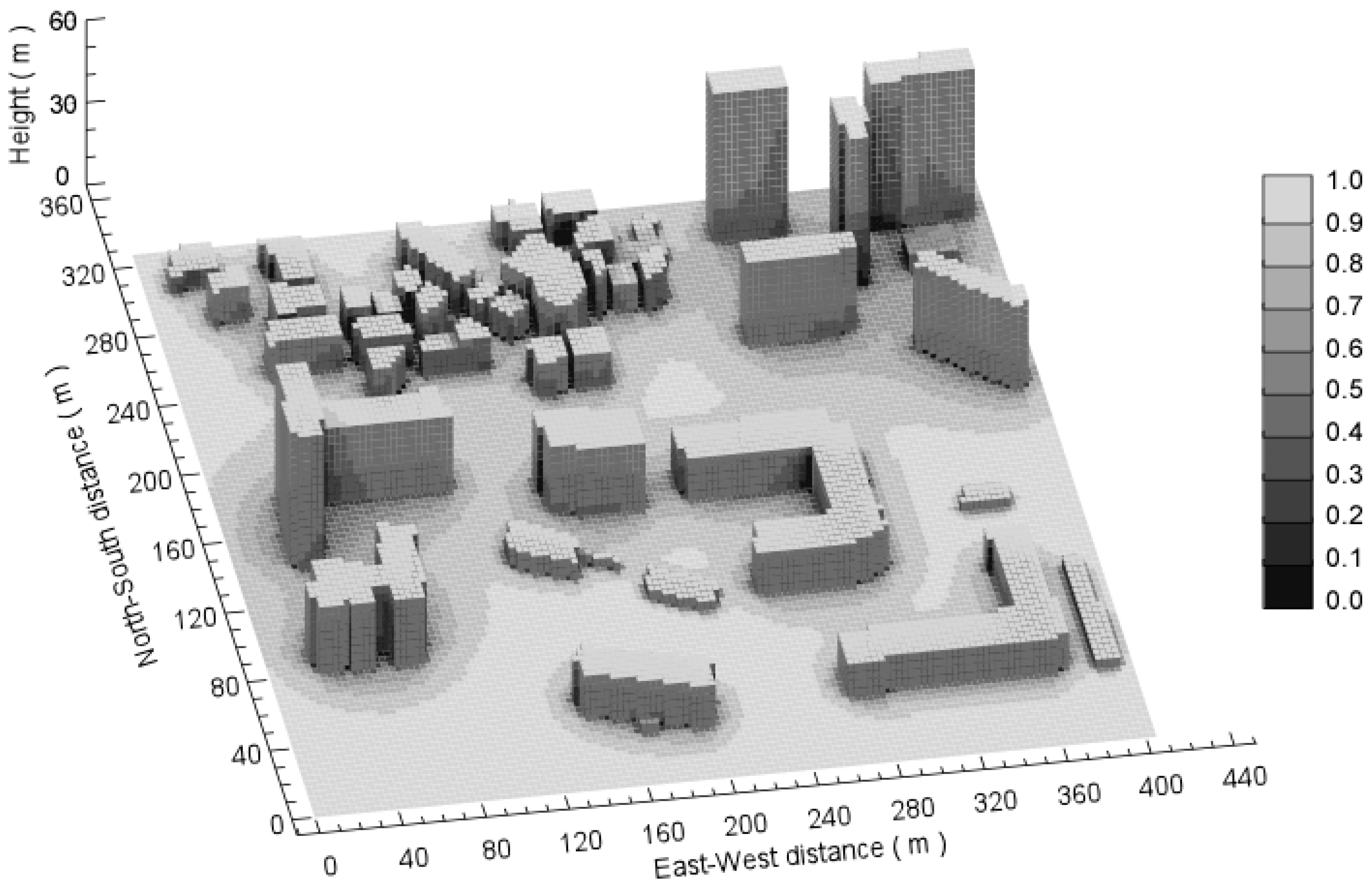
The simulation domain of the MUSE model configures with a 138 × 112 × 18 grid, which covers 414 × 336 m2 horizontally and 54 m vertically with the same grid resolution of 3 m (Figure 5b). The resultant total number of active patches is 24,323 in the simulation domain. The physical property parameters of each patch have been assigned according to the surface features of the real urban area. The aerodynamic roughness lengths for momentum are 0.05 m for roof and road patches, and the roughness lengths for heat are 0.0005 m for roof patches and 0.005 m for road patches. The radiative and thermal parameters of roof and wall patches are assigned for concrete and red brick, and those of road patches are for asphalt [64,70]. Table 3 summarizes the physical property parameters assigned for the real urban simulation. The roof, wall, and road patches are 0.5, 0.4, and 1.0 m in depth, configuring with ten sublayers at each patch. Each surface’s depth was determined based on the previous simulation studies that showed reasonable comparison against measurements (e.g., [64]).
The tower measurements are used to provide accurate meteorological forcing for validation of the MUSE model. The global shortwave and longwave radiative fluxes ( S d i r , S d i f , and L d i f ) from a four-component radiometer (CNR4, Campbell Scientific Inc., Cache Valley, UT, USA) deployed at the meteorological tower are applied homogeneously to the active patches, in which the measured global shortwave radiative flux is partitioned to the direct and the diffuse radiative fluxes following the empirical method [43,71]. The wind speed ( U a ) and air temperature ( T a ) adjacent to the active patches are obtained with interpolation from the wind speed and air temperature profiles computed using the flux measurements from the three-dimensional sonic anemometer (CSAT3, Campbell Scientific Inc., USA) and the Monin–Obukhov similarity relations as follows:
U ( z ) = u * κ [ ln ( z z 0 ) ψ m ( z L ) ] ,
T ( z ) = T o b s T * κ [ ln ( z o b s z ) ψ h ( z o b s L ) + ψ h ( z L ) ] ,
where U ( z ) and T ( z ) are the wind speed and air temperature at height z , respectively, T o b s is the air temperature measured at the height z o b s (=33 m a.g.l.). u * , T * , and L are the friction velocity, the surface-layer temperature scale, and the Obukhov length, which were measured directly from the flux tower. The aerodynamic roughness length is set to 1.06 m following the simple formulation of Grimmond and Oke [72] from the analysis of the site measurement [69], and the integrated stability functions for momentum ( ψ m ) and heat ( ψ h ) are given in Högström’s work ([73] and [74], respectively). The estimated wind speed and air temperature profiles are then horizontally interpolated to the model grid homogeneously as a meteorological forcing.
In this study, the CFD model developed by Kim et al. [75] is used to force the MUSE model. The model is simultaneously configured with a 138 × 112 × 19 grid using the same grid resolution of the MUSE model based on the Arakawa-C type grid system, which is adopted frequently in many CFD and LES models (e.g., [3,65]). These grid configurations make the MUSE model directly compatible with the micrometeorological models and available “online” and “offline” mode computation. Here, the CFD model ran with the estimated wind speed profile under the assumption of neutral atmospheric stratification, and the resultant wind fields were used as meteorological forcing of the MUSE model. The wind fields simulated by the CFD model are more realistic in spatial distribution over the simulation domain than the homogeneously distributed wind speed profile.
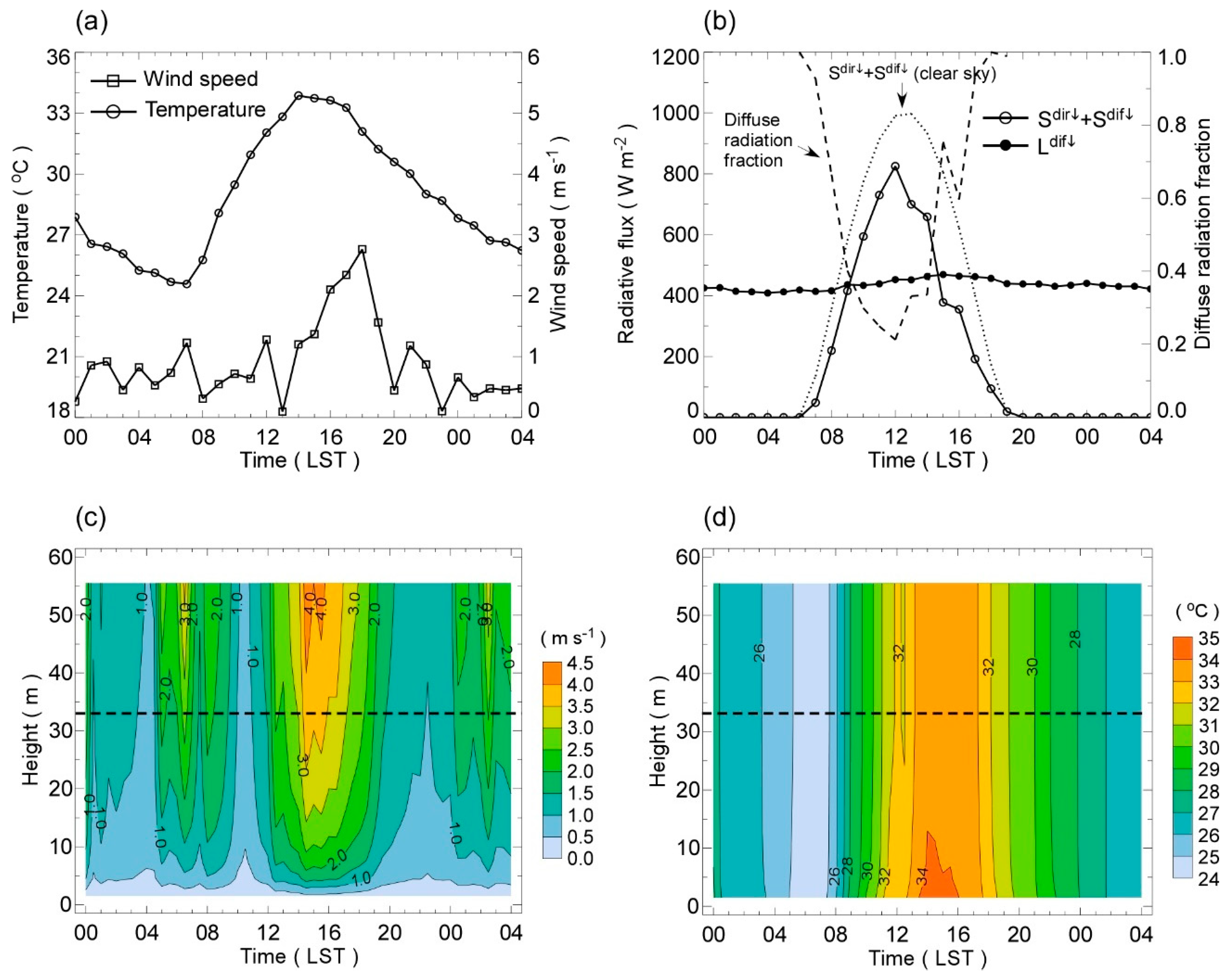
The MUSE validation simulation was conducted for 28 h from 00 LST 19 August to 04 LST 20 August 2016. The surface temperatures of every active patch were initialized from the spin-up simulation of the previous 18 days. The validation simulation marched with the time step of 5 sec and took approximately 25 min using a single CPU. Figure 6 shows diurnal variations of the meteorological forcing applied for the MUSE validation simulation. The air temperatures measured at 33 m a.g.l. ranged diurnally from 24.6 °C to 33.9 °C, and the nocturnal temperatures stayed above 26.2 °C (a tropical night) on 20 August 2016. The wind speed measured at 33 m a.g.l. remained quite low throughout the day, mostly ranging 0.5–1.0 m s−1 (Figure 6a). The low wind speed was found frequently in forming the surface layer on a hot summer day. The downward shortwave radiation reached approximately 825 W m−2 around noon, but it was influenced by clouds observed during the measurement on the day (Figure 6b). The wind speed and air temperature profiles estimated from the measurements show characteristic diurnal variations within the surface layer on the day (Figure 6c,d). The wind speeds are quite low near the ground throughout the day, which gradually increases with height. The air temperature profiles are relatively homogeneous in the vertical direction during the night, which indicates that the atmosphere remained near neutral or weakly unstable.

4. Validation Results

4.1. Shadow Model, View Factors, and Effective Albedos

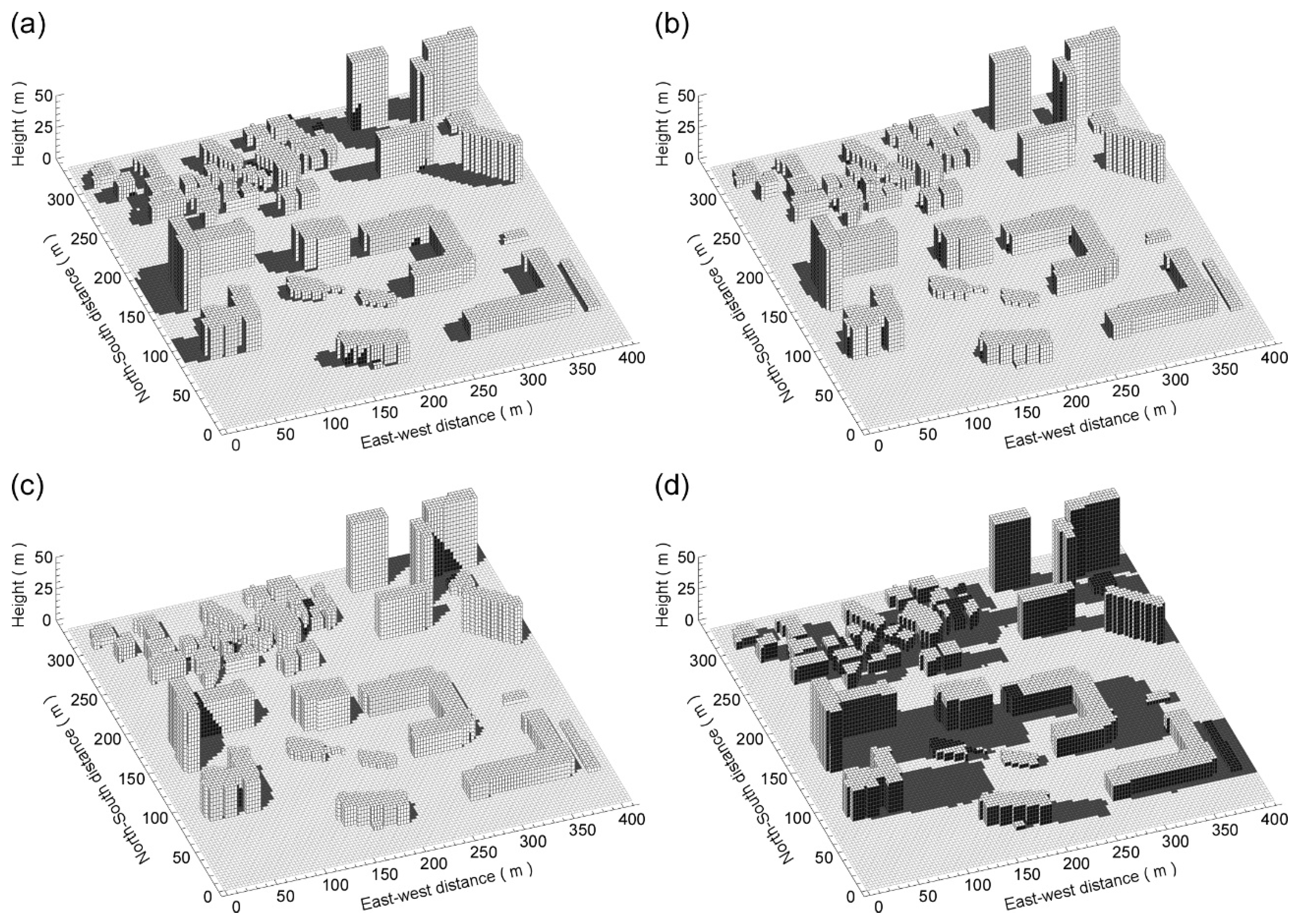
Figure 7 shows the spatial distributions of the sunlit/shaded patches estimated by the shadow model at different times of the day on 19 August 2016. The shaded areas vary depending on building geometries and the solar position, and the shadow model well represents the local shadow variation of each building and spatial distributions. At 09 LST, each building makes a shadow on the road patches and the wall patches on other frontal buildings. The shadow by the own building (“self-shading”) is also clearly simulated (Figure 7a). Around noon, more urban patches are sunlit with shorter shadow lengths according to the increase in solar altitude angle (Figure 7b,c). The shaded patches increase again in the late afternoon (Figure 7d). Because the shadow model determines the shadow distribution analytically based on building geometry and relative position of the sun, the computation uncertainty depends only on the representation accuracy of buildings’ geometries via grid resolution. The results show that the shadow model is capable of representing time-varying shadow geometries in complex real urban environments.
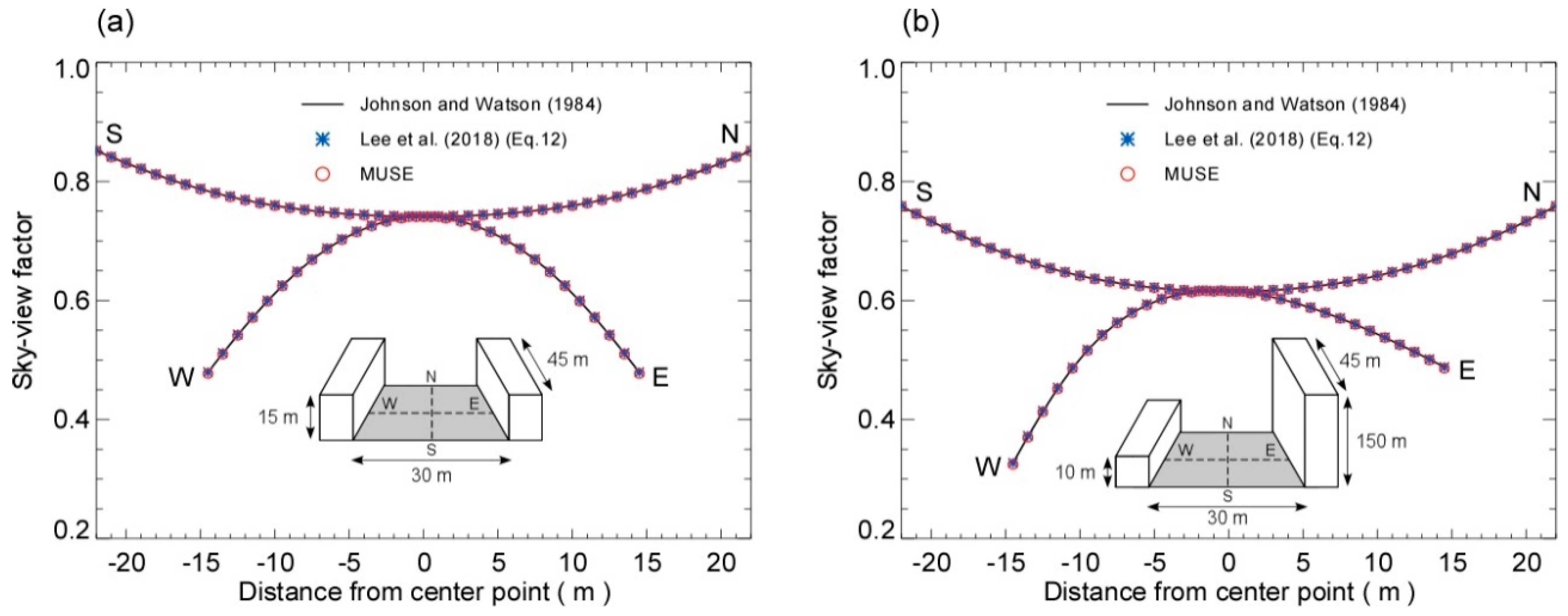
The analytical sky view factors calculated for ideal symmetrical and nonsymmetrical street canyon geometries can validate the computation method of the patch view factors in Section 2.2.2 (Figure 8). The symmetrical street canyon has the building height (H) of 15 m, the canyon width (W) of 30 m, and the canyon length (L) of 45 m (Figure 8a), while the nonsymmetrical street canyon has the two asymmetric building heights of 10 and 150 m, the canyon width of 30 m, and the canyon length of 45 m (Figure 8b). The MUSE model computes the patch view factors with a grid spacing of 1 m for both the street canyons. Meanwhile, the formulation of Johnson and Watson [59] gives the analytical sky view factors for validation. Figure 8 compares the numerical and analytical patch–sky view factors for the different geometric canyons. The sky view factors on the street canyon gradually decrease across the street canyon and increase along the street canyon with the distance from the canyon center. The patch–sky view factors at the higher building side are higher for the nonsymmetrical street canyon (Figure 8b). The MUSE model agrees well with the analytical patch–sky view factors at all the patches on both the symmetrical and nonsymmetrical street canyons. The formulations of Lee et al. [63] (Equations (12) and (15) in their paper) showed excellent agreement with the relative errors of less than 0.2% in the average sky view factor for the ideal street canyons, but they are applicable only for computing the sky view factors. The MUSE model shows a better agreement with relative errors of only less than 0.1% (Table 4). The MUSE model’s high accuracy stems from the formulations derived based on analytical relations [63]. Note that because the method’s error can increase with patch size and short distance, the computation of the view factors for two adjacent patches was calculated by dividing the adjacent patches into 3 × 3 subpatches.
Figure 9 presents the spatial distribution of the patch–sky view factors computed for the real urban area. The patch–sky view factors at horizontal patches have values ranging from 0 to 1, whereas the patch–sky view factors at vertical wall patches have values ranging from 0 up to 0.5. It shows that the patch–sky view factors vary significantly over the domain by representing the complicated building morphology. The patch–sky view factor is low in dense building areas while it is relatively high on the roof patches and open ground areas. Tall buildings influence the surrounding low-rise buildings by reducing the sky view factors. As the MUSE model can calculate the patch view factors on an analytical level of accuracy for the idealized urban geometries (Table 4), the computation uncertainty for the real urban area is only associated with the representation accuracy of buildings’ geometries, showing the capability of the MUSE model in determining the patch view factors for real urban environments.
The effective albedo, which is defined by the ratio of outgoing shortwave radiation to incident shortwave radiation, is an appropriate parameter for validation of the shortwave radiative processes within urban canyons, including radiative trapping effects discussed in Section 2.2.3. The experimental study of Aida [76] is used for the validation, which has been applied in many previous studies (e.g., [40,67,77,78]). In the experimental study, ideal canyon structures (“model”) of the north-south canyon model (“model 1”) and the east-west canyon model (“model 2”), and the cubed array canyon model (“model 3”) were set up using cubed concrete blocks with height and width of 0.15 m. The effective albedo was measured at 0.45 m high using pyranometers. The MUSE model is applied for the experimental data obtained on a summer day (15 June 1978) and a winter day (3 December 1977) to the three different canyon geometries, which are configured with the same size of blocks as in Aida [76] experiments. The block surface albedos of wall and ground surfaces are assigned by 0.4 following Aida [76], but the rooftop and road surface albedos are assigned to vary diurnally according to an empirical correction relation of the albedo following Sievers and Zdunkowski [77]. It was found that the surface albedo varied with the altitude of the sun due to the angular dependency of surface reflectivity in the experiment for the flat surface model (“model 0”) (Figure 10a,b). However, the MUSE model can not capture the angular dependency because it assumes Lambertian isotropic surface reflection. Therefore, the empirical corrections of the flat surface albedos were applied for validation purposes. The downward shortwave radiation and its partitioning into the direct and diffuse shortwave radiation are calculated based on empirical formulas in Overby et al. [43] with clear-day atmospheric turbidity conditions in Monteith and Unsworth [71].
The temporal variations of the effective albedos simulated for the three canyon geometries compare well with the measurements, showing that the MUSE model captures the characteristic temporal variations measured at the three canyon geometries in different seasons (Figure 10c–h). It has the temporal correlation coefficients of 0.69–0.99 for the summer day and 0.85–0.92 for the winter day. The relatively low correlation found in model 3 may attribute to the fact that the variation of the measured effective albedos is flat during the daytime. Meanwhile, the mean absolute errors of the simulated effective albedos are 0.002–0.016 for the summer day and 0.009–0.014 for the winter day, which corresponds to only 0.6–5.5% errors against the measurements (Table 5). It implies that the model errors are almost within the measurement accuracy (~5%).

4.2. The Real Urban Simulation

The model’s performance in simulating surface temperatures and surface energy balance fluxes in real urban environments was tested against the measurements obtained from the Kongju National University area on a hot summer day. Figure 11 demonstrates spatial distributions of the simulated surface temperatures at different times of the day. It shows that the MUSE model can capture the evolution of spatial and temporal variations of the surface temperatures on each patch level. The simulated surface temperatures range spatially by 34 ± 4 °C at 09 LST, 49 ± 12 °C at 12 LST, 49 ± 10 °C at 15 LST, and 39 ± 5 °C at 18 LST. The surface temperatures and their spatial heterogeneities are relatively high around noon, as was discussed in Kim et al. [75]. Relatively lower surface temperatures are found at self-shaded walls and densely built-up areas, whereas the open patches such as rooftops and broad roads have relatively higher surface temperatures. These temporal and spatial variations are closely correlated with the solar radiation amount reaching the patches, suggesting the importance of accurate representation of the radiative processes in the model.
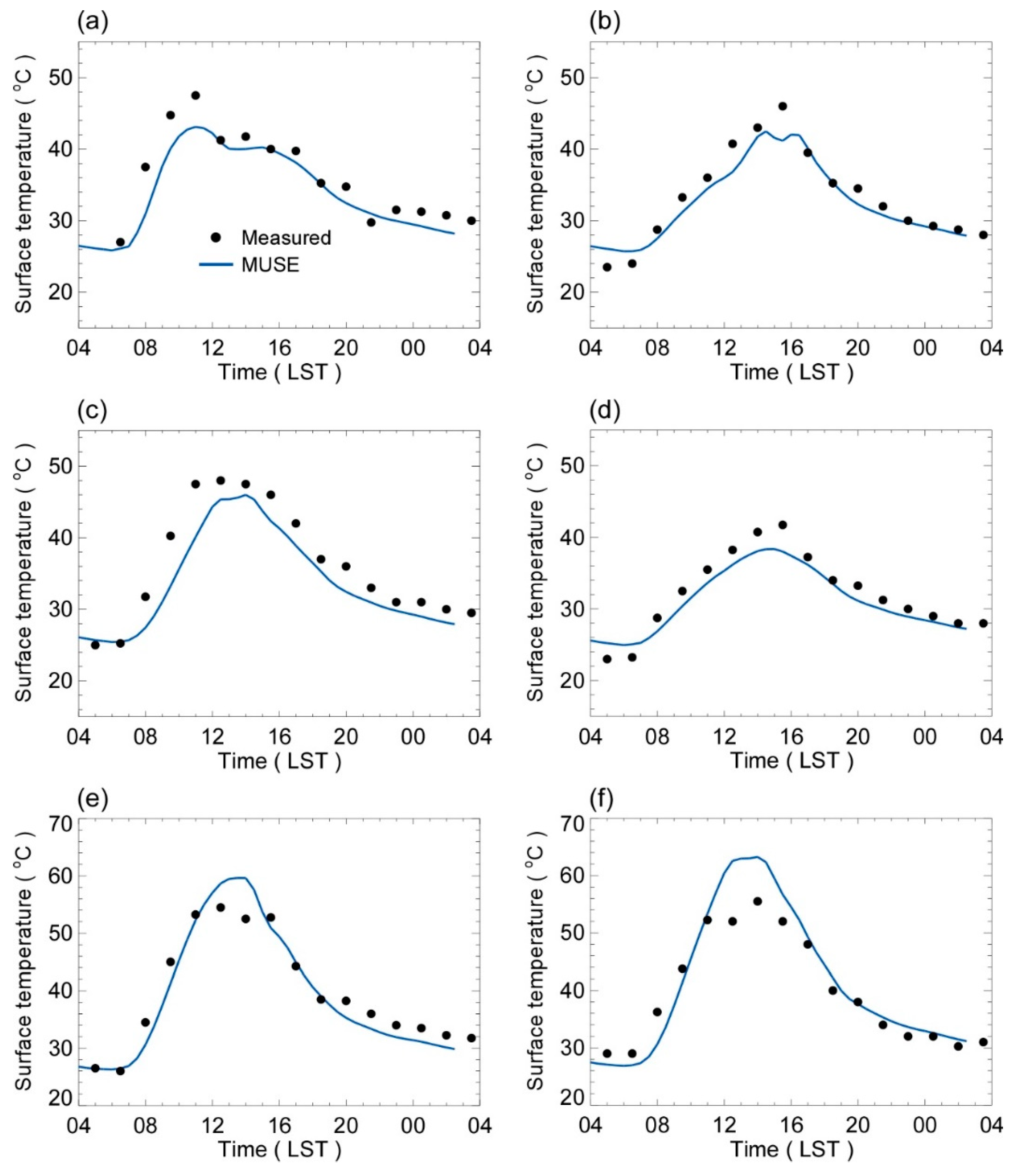
Figure 12 compares the diurnal variations of the simulated surface temperatures against the field measurements at the roof, road, and four walls surfaces. The wall surface temperature has a characteristic diurnal variation according to its facing orientation (Figure 12a–d). The sun begins to heat the east wall first in the morning, and it heats the south and west walls in order as time goes on. The north wall has the smallest diurnal variation as expected. The roof and road surface temperatures have relatively higher surface temperatures due to their openness (Figure 12e,f). The model tends to slightly underestimate the wall temperatures while it overestimates the peak temperatures at the roof and road surfaces. The model measurement discrepancies might attribute to many aspects associated with the physical processes such as radiation, turbulent heat exchange, and subsurface heat storage, but they are not quantitatively discernible in this study. The surface temperatures simulated by the MUSE model compare well with the measurements, capturing the characteristic temporal patterns at the six different patch surfaces with correlation coefficients in the range of 0.94–0.98. The statistical evaluation results show that the mean bias errors (MBE) are only less than 3 °C and the root mean square errors (RMSE) are in the range of approximately 2–4 °C (Table 6).
Figure 13 compares the diurnal variations of the simulated surface energy balance fluxes against the flux tower measurements at the urban site, and the statistical evaluation results are given in Table 7. The MUSE model underestimates the measured net radiation by MBE of −50.52 W m−2, while it overestimates the storage heat fluxes by MBE of −49.33 W m−2. The simulated turbulent heat fluxes are relatively well compared with the measurement with MBE of −1.69 W m−2. The statistical analysis shows that the model biases are systematic from the ratio of RMSEs to RMSE by 85% and 61% both in net radiation and storage heat flux, respectively. The temporal correlation coefficients are high—0.99 and 0.96 for net radiation and storage heat flux, respectively. These results imply that the model measurement discrepancies might be associated with static surface physical properties over the domain, such as surface albedo and thermal heat capacity. Despite the discrepancies, the MUSE model reproduces the surface energy balance over the area. The measured and simulated ratios of the storage heat flux to net radiation (G/R*) are about 0.72 and 0.69 during the daytime (0800-1600 LST) and 1.06 and 1.13 at night (2000-0200 LST), respectively. The relatively high G/R* is a characteristic feature of the heatwave period associated with weak winds in the urban area. Overall the MUSE model simulates diurnal variations of the surface fluxes and the relative energy balance measured in the urban area.

5. Summary and Conclusions

The MUSE model that is capable of representing the urban physical processes and their interactions in complex urban surfaces, and that can be compatible easily with general Cartesian grid microscale atmospheric models, was developed, which was coded in Fortran. The model represents complex urban surface morphology using three-dimensional patch surfaces, and it solves the urban physical processes of shortwave and longwave radiative transfers, turbulent exchanges of momentum and heat, and conductive heat transfer into urban subsurfaces. A shadow submodel is embedded to calculate time-varying shadow distributions in general urban environments, and the analytically-based numerical formulation is applied to estimate three-dimensional patch view factor distributions. The Monin–Obukhov similarity relation and the empirical formulation is used for turbulent heat exchanges on the horizontal (roofs and roads) and vertical wall surfaces, respectively. The conductive heat transfer at every patch is calculated based on Fourier’s law. The MUSE model solves all of the urban physical processes interactively during the time integration and applies computationally efficient treatments for real urban applications.
We evaluated the MUSE model in terms of all of the model’s physical processes and the full capability for use in a real urban environment. The embedded physical processes’ validation results showed that the model could compute three-dimensional building shadows, patch view factors, and the urban radiative transfers for ideal urban geometries on a high accuracy level comparable to analytic solutions or measurement errors. The model’s full capability was validated against the field measurements in simulating three-dimensional surface temperatures and surface energy balance fluxes at the Kongju National University campus area on a 3-m grid resolution. It first demonstrated that the model could reproduce the three-dimensional distributions of building shadows and patch view factors reflecting the urban area’s morphological features. The simulation results showed that the surface thermal states changed significantly in space and time, and the model captured the thermal heterogeneities over the campus area. The MUSE model’s realistic reproduction might be attributed to the interactive parameterization of the urban physical processes in real urban environments. Overall, the validation results demonstrate potential capabilities of the MUSE model for use in real urban simulations, implying that the assumption of homogeneous surface forcing found frequently in microscale atmospheric modeling should be reconsidered for realistic urban flow and dispersion simulations.
Because the model grid structure was designed to be compatible directly with general Cartesian grid microscale atmospheric models, the MUSE model can be easily used with CFDs and LESs models. The validation simulation in this study showed the capability in providing the mechanical forcing of every patch over the domain. The integrated modeling frame will be useful in interpreting various urban atmospheric and environmental problems (e.g., ventilation, heatwave, air quality) in real urban environments (e.g., [75,79]). For example, Kim et al. [75] examined the ventilation and thermal discomfort in a highly urbanized area using the CFD and MUSE coupled model.
As most CFD and LES models that have been used in urban microscale modeling have been developed based on a Cartesian coordinate, all the buildings in MUSE are thus represented by E-W and N-S parallel patches accordingly in this study, and the current realization of the MUSE formulation is limited to only horizontal and vertical surfaces. Realistic representation of slope surfaces and associated physical processes will be necessary for more realistic simulation, and the MUSE formulation given in this study can be applied to slope surfaces as well in calculation of shadow, view factor, and associated physical processes. The urban vegetation and associated hydrological processes are also important meteorological and environmental ingredients (e.g., [64,79,80]). Further development of the MUSE model for a better representation of real urban surfaces is currently underway.

Author Contributions

Conceptualization, S.-H.L.; methodology, D.-I.L. and S.-H.L.; formal analysis, D.-I.L. and S.-H.L.; writing—original draft preparation, D.-I.L. and S.-H.L.; writing—review and editing, S.-H.L.; visualization, D.-I.L.; funding acquisition, S.-H.L. All authors have read and agreed to the published version of the manuscript.

Funding

This work was supported by the Korea Meteorological Administration Research and Development Program (grant number: KMI2018-05611) and the National Research Foundation of Korea (NRF) grant funded by the Korea government (MEST) (grant number: 2017R1A2B4012975).

Acknowledgments

The authors are grateful to three anonymous reviewers for their valuable comments.

Conflicts of Interest

The authors declare no conflict of interest.

Appendix A. Comparison of the MUSE and TUF-3D Models

Table A1. The physical and numerical parameterizations of the MUSE and TUF-3D models.
MUSE
(This Study)
TUF-3D
(Krayenhoff et al. [40])
Shadow modelGeometric ray casting approach
(this study)
Ray tracing algorithm
(modified from Soux et al. [81])
View factorNumerical method based on analytical formulation
(Lee et al. [63])
Exact plane parallel analytical equations
(Siegel and Howell [57])
Turbulent sensible heat exchange for roof and road surfacesMonin–Obukhov similarity
(Lee and Park [64])
Empirical formulation
(Rowley et al. [66]; Cole and Sturrock [82])
Turbulent sensible heat exchange for wall surfacesEmpirical formulation
(Rowley et al. [66])
Empirical formulation
(Rowley et al. [66]; Cole and Sturrock [82])
Subsurface heat conduction1-D heat conduction equation/explicit finite difference method on a staggered grid
(Lee and Park [64])
1-D heat conduction equation/finite difference method on a regular grid
(Masson [67])

References

  1. Lee, I.Y.; Park, H.M. Parameterization of the pollutant transport and dispersion in urban street canyons. Atmos. Environ. 1994, 28, 2343–2349. [Google Scholar] [CrossRef]
  2. Baik, J.-J.; Kim, J.-J. A Numerical Study of Flow and Pollutant Dispersion Characteristics in Urban Street Canyons. J. Appl. Meteorol. 1999, 38, 1576–1589. [Google Scholar] [CrossRef]
  3. Baik, J.-J.; Kim, J.-J.; Fernando, H.J.S. A CFD Model for Simulating Urban Flow and Dispersion. J. Appl. Meteorol. 2003, 42, 1636–1648. [Google Scholar] [CrossRef]
  4. Kanda, M.; Moriwaki, R.; Kasamatsu, F. Large-Eddy Simulation of Turbulent Organized Structures within and above Explicitly Resolved Cube Arrays. Bound. Layer Meteorol. 2004, 112, 343–368. [Google Scholar] [CrossRef]
  5. Letzel, M.O.; Krane, M.; Raasch, S. High resolution urban large-eddy simulation studies from street canyon to neighbourhood scale. Atmos. Environ. 2008, 42, 8770–8784. [Google Scholar] [CrossRef]
  6. Inagaki, A.; Castillo, M.C.L.; Yamashita, Y.; Kanda, M.; Takimoto, H. Large-Eddy Simulation of Coherent Flow Structures within a Cubical Canopy. Bound. Layer Meteorol. 2012, 142, 207–222. [Google Scholar] [CrossRef]
  7. Kim, J.-J.; Baik, J.-J. A Numerical Study of Thermal Effects on Flow and Pollutant Dispersion in Urban Street Canyons. J. Appl. Meteorol. 1999, 38, 1249–1261. [Google Scholar] [CrossRef]
  8. Lin, M.; Hang, J.; Li, Y.; Luo, Z.; Sandberg, M. Quantitative ventilation assessments of idealized urban canopy layers with various urban layouts and the same building packing density. Build. Environ. 2014, 79, 152–167. [Google Scholar] [CrossRef]
  9. Ramponi, R.; Blocken, B.; De Coo, L.B.; Janssen, W.D. CFD simulation of outdoor ventilation of generic urban configurations with different urban densities and equal and unequal street widths. Build. Environ. 2015, 92, 152–166. [Google Scholar] [CrossRef] [Green Version]
  10. Hang, J.; Li, Y.; Sandberg, M.; Buccolieri, R.; Di Sabatino, S. The influence of building height variability on pollutant dispersion and pedestrian ventilation in idealized high-rise urban areas. Build. Environ. 2012, 56, 346–360. [Google Scholar] [CrossRef]
  11. Blocken, B.; Janssen, W.; Van Hooff, T. CFD simulation for pedestrian wind comfort and wind safety in urban areas: General decision framework and case study for the Eindhoven University campus. Environ. Model. Softw. 2012, 30, 15–34. [Google Scholar] [CrossRef]
  12. Park, S.-B.; Baik, J.-J.; Lee, S.-H. Impacts of Mesoscale Wind on Turbulent Flow and Ventilation in a Densely Built-up Urban Area. J. Appl. Meteorol. Clim. 2015, 54, 811–824. [Google Scholar] [CrossRef]
  13. Shi, X.; Zhu, Y.; Duan, J.; Shao, R.; Wang, J. Assessment of pedestrian wind environment in urban planning design. Landsc. Urban Plan. 2015, 140, 17–28. [Google Scholar] [CrossRef]
  14. Antoniou, N.; Montazeri, H.; Wigo, H.; Neophytou, M.K.-A.; Blocken, B.; Sandberg, M. CFD and wind-tunnel analysis of outdoor ventilation in a real compact heterogeneous urban area: Evaluation using “air delay”. Build. Environ. 2017, 126, 355–372. [Google Scholar] [CrossRef]
  15. Kurppa, M.; Hellsten, A.; Auvinen, M.; Raasch, S.; Vesala, T.; Järvi, L. Ventilation and Air Quality in City Blocks Using Large-Eddy Simulation—Urban Planning Perspective. Atmosphere 2018, 9, 65. [Google Scholar] [CrossRef] [Green Version]
  16. Toparlar, Y.; Blocken, B.; Maiheu, B.; Van Heijst, G.J. A review on the CFD analysis of urban microscale. Renew. Sustain. Energy Rev. 2017, 80, 1613–1640. [Google Scholar] [CrossRef]
  17. Gál, T.; Unger, J. A new software tool for SVF calculations using building and tree-crown databases. Urban Clim. 2014, 10, 594–606. [Google Scholar] [CrossRef] [Green Version]
  18. Tamura, T. Towards practical use of LES in wind engineering. J. Wind Eng. Ind. Aerodyn. 2008, 96, 1451–1471. [Google Scholar] [CrossRef]
  19. Letzel, M.O.; Helmke, C.; Ng, E.; An, X.; Lai, A.; Raasch, S. LES case study on pedestrian level ventilation in two neighbourhoods in Hong Kong. Meteorol. Z. 2012, 21, 575–589. [Google Scholar] [CrossRef]
  20. Park, S.-B.; Baik, J.-J.; Han, B.-S. Large-eddy simulation of turbulent flow in a densely built-up urban area. Environ. Fluid Mech. 2013, 15, 235–250. [Google Scholar] [CrossRef]
  21. Kanda, M.; Inagaki, A.; Miyamoto, T.; Gryschka, M.; Raasch, S. A new aerodynamic parameterization for real urban surfaces. Bound. Layer Meteorol. 2013, 148, 357–377. [Google Scholar] [CrossRef]
  22. Nakayama, H.; Jurčáková, K.; Nagai, H. Large-Eddy Simulation of plume dispersion within various actual urban areas. Adv. Sci. Res. 2013, 10, 33–41. [Google Scholar] [CrossRef] [Green Version]
  23. Scherer, D.; Fehrenbach, U.; Fenner, D.; Grassmann, T.; Holtmann, A.; Krug, A.; Meier, F.; Otto, M.; Scherber, K. Overview on multi-scale, three-dimensional atmospheric studies in Berlin, Germany. In Proceedings of the 10th International Conference on Urban Climate/14th Symposium on the Urban Environment, New York, NY, USA, 6–10 August 2018. [Google Scholar]
  24. Gowardhan, A.A.; Pardyjak, E.R.; Senocak, I.; Brown, M.J. A CFD-based wind solver for an urban fast response transport and dispersion model. Environ. Fluid Mech. 2011, 11, 439–464. [Google Scholar] [CrossRef]
  25. Kim, J.-J.; Baik, J.-J. Urban street-canyon flows with bottom heating. Atmos. Environ. 2001, 35, 3395–3404. [Google Scholar] [CrossRef]
  26. Kovar-Panskus, A.; Moulinneuf, L.; Savory, E.; Abdelqari, A.; Sini, J.-F.; Rosant, J.-M.; Robins, A.; Toy, N. A Wind Tunnel Investigation of the Influence of Solar-Induced Wall-Heating on the Flow Regime within a Simulated Urban Street Canyon. Water Air Soil Pollut. Focus 2002, 2, 555–571. [Google Scholar] [CrossRef]
  27. Xie, X.; Liu, C.-H.; Leung, D.Y.C.; Leung, M.K.H. Characteristics of air exchange in a street canyon with ground heating. Atmos. Environ. 2006, 40, 6396–6409. [Google Scholar] [CrossRef]
  28. Kwak, K.-H.; Baik, J.-J.; Lee, S.-H.; Ryu, Y.-H. Computational Fluid Dynamics Modelling of the Diurnal Variation of Flow in a Street Canyon. Bound. Layer Meteorol. 2011, 141, 77–92. [Google Scholar] [CrossRef]
  29. Yang, L.; Li, Y. Thermal conditions and ventilation in an ideal city model of Hong Kong. Energy Build. 2011, 43, 1139–1148. [Google Scholar] [CrossRef]
  30. Cai, X.M. Effects of Wall Heating on Flow Characteristics in a Street Canyon. Bound. Layer Meteorol. 2012, 142, 443–467. [Google Scholar] [CrossRef]
  31. Santiago, J.L.; Krayenhoff, E.S.; Martilli, A. Flow simulations for simplified urban configurations with microscale distributions of surface thermal forcing. Urban Clim. 2014, 9, 115–133. [Google Scholar] [CrossRef]
  32. Nazarian, N.; Kleissl, J. Realistic solar heating in urban areas: Air exchange and street-canyon ventilation. Build. Environ. 2016, 95, 75–93. [Google Scholar] [CrossRef] [Green Version]
  33. Nazarian, N.; Martilli, A.; Kleissl, J. Impacts of Realistic Urban Heating, Part I: Spatial Variability of Mean Flow, Turbulent Exchange and Pollutant Dispersion. Bound. Layer Meteorol. 2017, 166, 367–393. [Google Scholar] [CrossRef]
  34. Nazarian, N.; Martilli, A.; Norford, L.; Kleissl, J. Impacts of realistic urban heating, part Ⅱ: Air quality and city breathability. Bound. Layer Meteorol. 2018, 168, 321–341. [Google Scholar] [CrossRef] [Green Version]
  35. Wang, W.; Ng, E. Air ventilation assessment under unstable atmospheric stratification—A comparative study for Hong Kong. Build. Environ. 2018, 130, 1–13. [Google Scholar] [CrossRef] [PubMed]
  36. Roth, M.; Oke, T.R.; Emery, W.J. Satellite-derived urban heat islands from three coastal cities and the utilization of such data in urban climatology. Int. J. Remote Sens. 1989, 10, 1699–1720. [Google Scholar] [CrossRef]
  37. Voogt, J.A.; Oke, T.R. Effects of urban surface geometry on remotely-sensed surface temperature. Int. J. Remote Sens. 1998, 19, 895–920. [Google Scholar] [CrossRef]
  38. Voogt, J.A.; Oke, T.R. Thermal remote sensing of urban climates. Remote Sens. Environ. 2003, 86, 370–384. [Google Scholar] [CrossRef]
  39. Hu, L.; Monaghan, A.; Voogt, J.A.; Barlage, M. A first satellite-based observational assessment of urban thermal anisotropy. Remote Sens. Environ. 2016, 181, 111–121. [Google Scholar] [CrossRef] [Green Version]
  40. Krayenhoff, E.S.; Voogt, J.A. A microscale three-dimensional urban energy balance model for studying surface temperatures. Bound. Layer Meteorol. 2007, 123, 433–461. [Google Scholar] [CrossRef]
  41. Yaghoobian, N.; Kleissl, J. An indoor–outdoor building energy simulator to study urban modification effects on building energy use—Model description and validation. Energy Build. 2012, 54, 407–417. [Google Scholar] [CrossRef]
  42. Yang, X.; Li, Y. Development of a Three-Dimensional Urban Energy Model for Predicting and Understanding Surface Temperature Distribution. Bound. Layer Meteorol. 2013, 149, 303–321. [Google Scholar] [CrossRef]
  43. Overby, M.; Willemsen, P.; Bailey, B.N.; Halverson, S.; Pardyjak, E.R. A rapid and scalable radiation transfer model for complex urban domains. Urban Clim. 2016, 15, 25–44. [Google Scholar] [CrossRef] [Green Version]
  44. Yaghoobian, N.; Kleissl, J.; Paw U, K.T. An Improved Three-Dimensional Simulation of the Diurnally Varying Street-Canyon Flow. Bound. Layer Meteorol. 2014, 153, 251–276. [Google Scholar] [CrossRef]
  45. Aliabadi, A.A.; Krayenhoff, E.S.; Nazarian, N.; Chew, L.W.; Armstrong, P.R.; Afshari, A.; Norford, L.K. Effects of Roof-Edge Roughness on Air Temperature and Pollutant Concentration in Urban Canyons. Bound. Layer Meteorol. 2017, 164, 249–279. [Google Scholar] [CrossRef]
  46. Yang, X.; Li, Y. The impact of building density and building height heterogeneity on average urban albedo and street surface temperature. Build. Environ. 2015, 90, 146–156. [Google Scholar] [CrossRef]
  47. Resler, J.; Krč, P.; Belda, M.; Juruš, P.; Benešová, N.; Lopata, J.; Vlček, O.; Damašková, D.; Eben, K.; Derbek, P.; et al. PALM-USM v1.0: A new urban surface model integrated into the PALM large-eddy simulation model. Geosci. Model Dev. 2017, 10, 3635–3659. [Google Scholar] [CrossRef] [Green Version]
  48. Núñez, M.; Oke, T.R. Modeling the Daytime Urban Surface Energy Balance. Geogr. Anal. 1980, 12, 373–386. [Google Scholar] [CrossRef]
  49. Oke, T.R.; Kalanda, B.D.; Steyn, D.G. Parameterization of heat storage in urban areas. Urban Ecol. 1981, 5, 45–54. [Google Scholar] [CrossRef]
  50. Doll, D.; Ching, J.K.S.; Kaneshiro, J. Parameterization of subsurface heating for soil and concrete using net radiation data. Bound. Layer Meteorol. 1985, 32, 351–372. [Google Scholar] [CrossRef]
  51. Anandakumar, K. A study on the partition of net radiation into heat fluxes on a dry asphalt surface. Atmos. Environ. 1999, 33, 3911–3918. [Google Scholar] [CrossRef]
  52. Smith, J.B.; Schellnhuber, H.J.; Mirza, M.M.; Frankhauser, S.; Leemans, R.; Erda, L.; Ogallo, L.; Pittock, B.; Richels, R.; Rosenzweig, C.; et al. Vulnerability to climate change and reasons for concern: A synthesis. In Climate Change 2001: Impacts, Adaptation, and Vulnerability; Cambridge University Press: Cambridge, UK; New York, NY, USA, 2001; pp. 913–967. [Google Scholar]
  53. Adebayo, Y.R. Aspects of the variation in some characteristics of radiation budget within the urban canopy of Ibadan. Atmos. Environ. Part B Urban Atmos. 1990, 24, 9–17. [Google Scholar] [CrossRef]
  54. Mills, G. An urban canopy-layer climate model. Theor. Appl. Clim. 1997, 57, 229–244. [Google Scholar] [CrossRef]
  55. Johnson, G.T.; Oke, T.R.; Lyons, T.J.; Steyn, D.G.; Watson, I.D.; Voogt, J.A. Simulation of surface urban heat islands under ‘IDEAL’ conditions at night part 1: Theory and tests against field data. Bound. Layer Meteorol. 1991, 56, 275–294. [Google Scholar] [CrossRef]
  56. Swaid, H. The role of radiative-convective interaction in creating the microclimate of urban street canyons. Bound. Layer Meteorol. 1993, 64, 231–259. [Google Scholar] [CrossRef]
  57. Siegel, R.; Howell, J.R. Thermal Radiation and Heat Transfer; McGraw-Hill: New York, NY, USA, 1972; p. 825. [Google Scholar]
  58. Oke, T.R. Canyon geometry and the nocturnal urban heat island: Comparison of scale model and field observations. J. Clim. 1981, 1, 237–254. [Google Scholar] [CrossRef]
  59. Johnson, G.T.; Watson, I.D. The Determination of View-Factors in Urban Canyons. J. Clim. Appl. Meteorol. 1984, 23, 329–335. [Google Scholar] [CrossRef]
  60. Zakšek, K.; Oštir, K.; Kokalj, Ž. Sky-View Factor as a Relief Visualization Technique. Remote Sens. 2011, 3, 398–415. [Google Scholar] [CrossRef] [Green Version]
  61. Krayenhoff, E.S.; Christen, A.; Martilli, A.; Oke, T.R. A Multi-layer Radiation Model for Urban Neighbourhoods with Trees. Bound. Layer Meteorol. 2014, 151, 139–178. [Google Scholar] [CrossRef]
  62. Wang, Z.-H. Monte Carlo simulations of radiative heat exchange in a street canyon with trees. Sol. Energy 2014, 110, 704–713. [Google Scholar] [CrossRef] [Green Version]
  63. Lee, D.-I.; Woo, J.-W.; Lee, S.-H. An analytically based numerical method for computing view factors in real urban environments. Theor. Appl. Clim. 2018, 131, 445–453. [Google Scholar] [CrossRef]
  64. Lee, S.-H.; Park, S.-U. A Vegetated Urban Canopy Model for Meteorological and Environmental Modelling. Bound. Layer Meteorol. 2008, 126, 73–102. [Google Scholar] [CrossRef]
  65. Maronga, B.; Gryschka, M.; Heinze, R.; Hoffmann, F.; Kananisuhring, F.; Keck, M.; Ketelsen, K.; Letzel, M.O.; Suhring, M.; Raasch, S. The Parallelized Large-Eddy Simulation Model (PALM) version 4.0 for atmospheric and oceanic flows: Model formulation, recent developments, and future perspectives. Geosci. Model Dev. 2015, 8, 2515–2551. [Google Scholar] [CrossRef] [Green Version]
  66. Rowley, F.B.; Algren, A.B.; Blackshaw, J.L. Surface conductances as affected by air velocity, temperature and character of surface. ASHRAE Trans. 1930, 36, 429–446. [Google Scholar]
  67. Masson, V. A Physically-Based Scheme For The Urban Energy Budget In Atmospheric Models. Bound. Layer Meteorol. 2000, 94, 357–397. [Google Scholar] [CrossRef]
  68. Oke, T.R. The urban energy balance. Prog. Phys. Geogr. Earth Environ. 1988, 12, 471–508. [Google Scholar] [CrossRef]
  69. Lee, D.-I.; Lee, J.-H.; Lee, S.-H. Uncertainty analysis of the eddy-covariance turbulence fluxes measured over a heterogeneous urban area: A coordinate tilt impact. Atmosphere 2016, 26, 473–482. [Google Scholar] [CrossRef] [Green Version]
  70. Lemonsu, A.; Grimmond, C.S.B.; Masson, V. Modeling the Surface Energy Balance of the Core of an Old Mediterranean City: Marseille. J. Appl. Meteorol. 2004, 43, 312–327. [Google Scholar] [CrossRef]
  71. Monteith, J.; Unsworth, M. Principles of Environmental Physics: Plants, Animals, and the Atmosphere, 3rd ed.; Academic Press: Waltham, MA, USA, 2008. [Google Scholar]
  72. Grimmond, C.S.B.; Oke, T.R. Aerodynamic Properties of Urban Areas Derived from Analysis of Surface Form. J. Appl. Meteorol. 1999, 38, 1262–1292. [Google Scholar] [CrossRef]
  73. Högström, U. Non-dimensional wind and temperature profiles in the atmospheric surface layer: A re-evaluation. Bound. Layer Meteorol. 1988, 42, 55–78. [Google Scholar] [CrossRef]
  74. Högström, U. Review of some basic characteristics of the atmospheric surface layer. Bound. Layer Meteorol. 1996, 78, 215–246. [Google Scholar] [CrossRef]
  75. Kim, D.-J.; Lee, D.-I.; Kim, J.-J.; Park, M.-S.; Lee, S.-H. Development of a Building-Scale Meteorological Prediction System Including a Realistic Surface Heating. Atmosphere 2020, 11, 67. [Google Scholar] [CrossRef] [Green Version]
  76. Aida, M. Urban albedo as a function of the urban structure? A model experiment. Bound. Layer Meteorol. 1982, 23, 405–413. [Google Scholar] [CrossRef]
  77. Sievers, U.; Zdunkowski, W. A numerical simulation scheme for the albedo of city street canyons. Bound. Layer Meteorol. 1985, 33, 245–257. [Google Scholar] [CrossRef]
  78. Sailor, D.J.; Fan, H. Modeling the diurnal variability of effective albedo for cities. Atmos. Environ. 2002, 36, 713–725. [Google Scholar] [CrossRef]
  79. Tsoka, S.; Tsikaloudaki, A.; Theodosiou, T. Analyzing the ENVI-met microclimate model’s performance and assessing cool materials and urban vegetation applications—A review. Sustain. Cities Soc. 2018, 43, 55–76. [Google Scholar] [CrossRef]
  80. Lee, S.-H.; Lee, H.; Park, S.-B.; Woo, J.-W.; Lee, D.-I.; Baik, J.-J. Impacts of in-canyon vegetation and canyon aspect ratio on the thermal environment of street canyons: Numerical investigation using a coupled WRF-VUCM model. Q. J. R. Meteorol. Soc. 2016, 142, 2562–2578. [Google Scholar] [CrossRef]
  81. Soux, A.; Voogt, J.A.; Oke, T.R. A Model to Calculate what a Remote Sensor ‘Sees’ of an Urban Surface. Bound. Layer Meteorol. 2004, 111, 109–132. [Google Scholar] [CrossRef]
  82. Cole, R.; Sturrock, N. The convective heat exchange at the external surface of buildings. Build. Environ. 1977, 12, 207–214. [Google Scholar] [CrossRef]
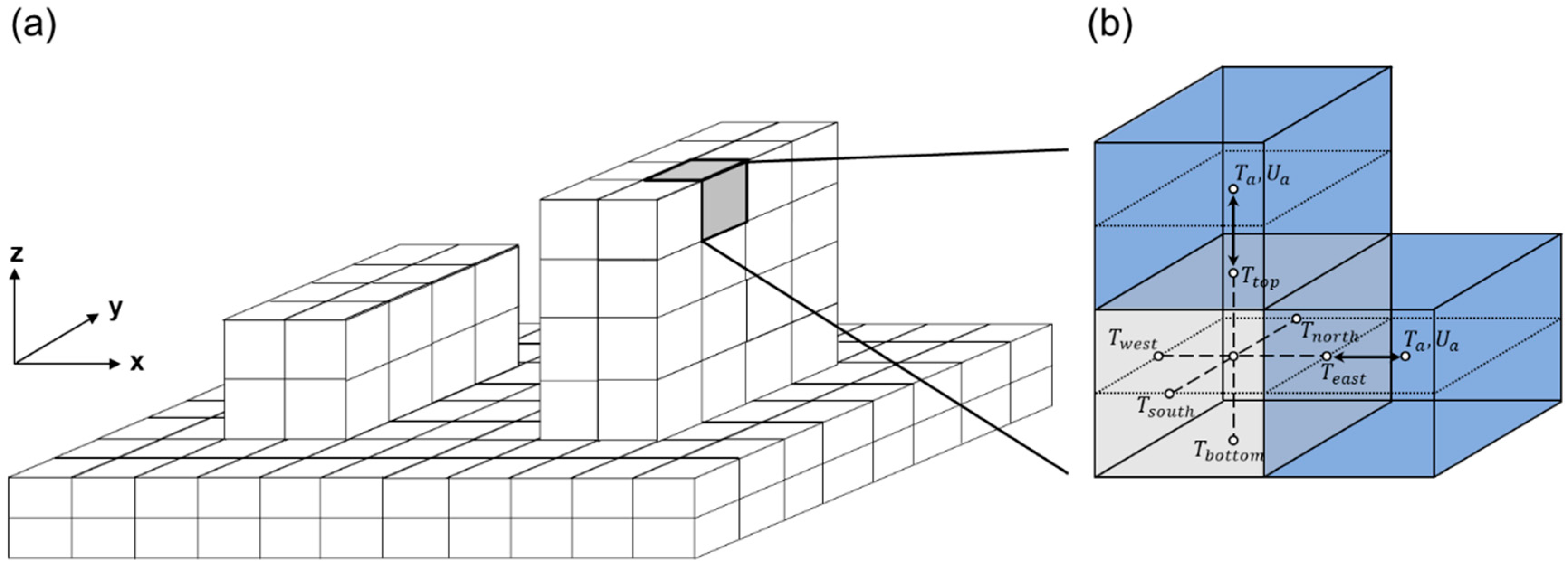
Figure 1. (a) Three-dimensional representation of urban buildings and ground surfaces in the microscale urban surface energy (MUSE) model. (b) Definition of the six patches (top, bottom, east, west, south, and north) and the active patches that interact with the surrounding atmospheric grid cells (blue). T a and U a are the air temperature and wind speed at the adjacent atmospheric grid cells, respectively.
Atmosphere 11 01347 g001
Figure 2. Configuration of the subsurface layers at each patch and associated physical processes in the MUSE model. T k , I denotes the subsurface temperature at the layer k of the patch I , and F k , I is the conductive heat flux at the vertical level k of the patch I . S d i r and S d i f denote the downward direct and diffuse shortwave radiation, respectively, and L d i f is the downward longwave radiation. T a and U a are the air temperature and wind speed at the adjacent atmospheric grid cells, respectively.
Atmosphere 11 01347 g002
Figure 3. Schematic of the shadow submodel of the MUSE model. It illustrates the shadow geometry formed by building A. Here, the shaded area denotes the actual shape of the building’s shadow calculated by the analytical computation, and the sol id line indicates the shaded patches estimated in the MUSE model. θ z and θ a are the solar zenith angle and the solar azimuth angle, respectively. l h o r and l v e r t are the horizontal shadow length and the vertical shadow length, respectively.
Atmosphere 11 01347 g003
Figure 4. Schematics of the patch–patch view factor computation for (a) ground–wall patches and (b) wall–wall patches (modified from Lee et al. [63]). Δ A I and Δ A J are the areas of the patches I and J , respectively. Δ X , Δ Y , and Δ Z are the distances between the two patches in each directions, and R is the distance between the two patches. n I and n J are the unit vectors perpendicular to the patches I and J , respectively.
Atmosphere 11 01347 g004
Figure 5. (a) The aerial view of the study area for the real urban environment test of the MUSE model (Source: Google Earth). The study area (36.4717° N, 127.1426° E) is located in the Kongju National University, South Korea, and a micrometeorological flux tower has been installed at the rooftop of a campus building (~33 m a.g.l.) (red circle). The surface temperatures were measured at the roof and wall surfaces of the building (red circle) and the road site (white circle). (b) The validation simulation domain and building height representation in the MUSE model. Each building height was represented using National Geographic Information System (NGIS) database from National Geographic Information Institute (NGII), Ministry of Land, Infrastructure and Transport (MLIT) of South Korea.
Atmosphere 11 01347 g005
Figure 6. Diurnal variations of the (a) air temperature and wind speed and the (b) downward shortwave and longwave radiation measured from the flux tower at the Kongju National University campus on 19 August 2016. The measured global shortwave radiation is partitioned to the direct ( S d i r ) and diffuse ( S d i f ) shortwave radiation according to the diffuse radiation fraction (dashed line in (b)) calculated following Overby et al. [43] and Monteith and Unsworth [71]. Time-height sections of the meteorological profiles of the (c) wind speed and (d) air temperature calculated from the meteorological and flux measurements at 33 m a.g.l. and the Monin–Obukhov similarity relation. The horizontal dashed line indicates the measurement height.
Atmosphere 11 01347 g006
Figure 7. Three-dimensional distributions of sunlit/shaded patches over the real urban area calculated by the shadow model at (a) 09 LST, (b) 12 LST, (c) 15 LST, and (d) 18 LST on 19 August 2016.
Atmosphere 11 01347 g007
Figure 8. Comparison of the patch–sky view factor ( ψ I s k y ) at horizontal patches estimated by the MUSE model and the analytical method (Johnson and Watson [59]) for (a) symmetrical finite length street canyon and (b) nonsymmetrical finite length street canyon. The computation by Equation (12) in Lee et al. [63] is also compared.
Atmosphere 11 01347 g008
Figure 9. Three-dimensional distribution of patch–sky view factors at each horizontal and vertical patch over the real urban area.
Atmosphere 11 01347 g009
Figure 10. Comparison of the observed and simulated effective albedos for the (a,b) flat surface, (c,d) north-south canyon model, (e,f) east-west canyon model, and (g,h) cube array canyon in the summer (left panels) and winter (right panels) experiment days. R is the correlation coefficient. The dotted line (ch) denotes the effective albedo computed without time-varying roof and road surface albedos.
Atmosphere 11 01347 g010
Figure 11. Three-dimensional distributions of the simulated surface temperatures at the horizontal and vertical patches over the real urban area at (a) 09 LST, (b) 12 LST, (c) 15 LST, and (d) 18 LST on 19 August 2016.
Atmosphere 11 01347 g011
Figure 12. Comparison of the measured and simulated surface temperatures of the (a) east wall, (b) west wall, (c) south wall, (d) north wall, (e) roof, and (f) road surface on 19 August 2016.
Atmosphere 11 01347 g012
Figure 13. Comparison of the measured and simulated net radiation (R*), turbulent heat fluxes (H), and storage heat fluxes (G) on 19 August 2016. The measured turbulent heat fluxes were calculated by the sum of sensible heat fluxes (H) and latent heat fluxes (L). The storage heat fluxes were estimated as a residual term between net radiation and turbulent heat fluxes.
Atmosphere 11 01347 g013
Table 1. Meteorological forcing variables and the predicted variables in the MUSE model.
VariableSymbolUnit
Meteorological forcing variablesWind velocity components U a ( U ,   V ,   W ) m s−1
Air temperature T a K
Downward direct shortwave radiation S d i r W m−2
Downward diffuse shortwave radiation S d i f W m−2
Downward longwave radiation L d i f W m−2
Predicted variablesFriction velocity u * m s−1
Incident direct shortwave radiation S I d i r W m−2
Incident diffuse shortwave radiation S I d i f W m−2
Reflected shortwave radiation S I R W m−2
Net shortwave radiation S I * W m−2
Emitted longwave radiation L I W m−2
Incident diffuse longwave radiation L I d i f W m−2
Reflected longwave radiation L I R W m−2
Net longwave radiatio L I R L I * W m−2
Sensible heat flux H I W m−2
Heat flux at subsurface layer k F k , I W m−2
Temperature at layer k T k , I K
Table 2. Physical property parameters of the MUSE model used to represent the physical properties of urban surfaces.
ParameterSymbolUnit
Roughness length for momentum z 0 m
Roughness length for heat z 0 T m
Surface albedo α -
Surface emissivity ε -
Thermal conductivity k W m−1 K−1
Volumetric heat capacity C J m−3 K−1
Thickness of each subsurface layer Δ z m
Table 3. Physical property parameters used for validation simulation of the Kongju National University campus site.
ParameterUnitRoofWallRoad
Roughness length for momentum ( z 0 )m0.05-0.05
Roughness length for heat ( z 0 T )m0.00005-0.00005
Surface albedo ( α )-0.280.200.18
Surface emissivity ( ε )-0.900.900.94
Thermal conductivity ( k )W m−1 K−10.900.700.79
Volumetric heat capacity ( C )J m−3 K−11.40 × 1061.60 × 1061.83 × 106
Thickness ( Δ z )m0.50.41.0
Table 4. Comparison of the average patch–sky view factors ( ψ I s k y ) estimated from the analytical formulation (Johnson and Watson [59]: JW84), the numerical method (Equation (12) in Lee et al. [63]: Lee18), and the MUSE model. Two different canyon geometries of the symmetrical and nonsymmetrical canyons are considered, and the patch–sky view factors calculated from each method are averaged across the street canyon (east-west direction), along the street canyon (north-south direction), and over the entire canyon surface. The value in parenthesis denotes the relative error (%) defined by ψ ψ J W 84 ψ J W 84 × 100 .
East-West DirectionNorth-South DirectionWhole Area
Symmetric canyonJW840.6460.7770.681
Lee180.647 (0.15)0.778 (0.12)0.682 (0.14)
MUSE0.645 (−0.07)0.777 (−0.01)0.681 (−0.06)
Asymmetric canyonJW840.5450.6630.589
Lee180.546 (0.14)0.664 (0.09)0.590 (0.14)
MUSE0.545 (−0.08)0.663 (−0.01)0.589 (−0.07)
Table 5. Comparison of mean absolute errors ( | α M O D α O B S | ) of the effective albedos ( α M O D ) from Sievers and Zdunkowski [77] (SZ95), TUF-3D, and the MUSE model against Aida’s experiment (Aida [76]) for two typical days of 15 June 1978 and 3 December 1977. The three different canyon geometries are model 1 (north-south canyon model), model 2 (west-east canyon model), and model 3 (2 × 2 cube array model). The value in parenthesis denotes the fractional error defined as | α M O D α O B S α O B S | × 100 .
15 June 19783 December 1977
Model 1Model 2Model 3Model 1Model 2Model 3
SZ850.015-0.020-
TUF-3D0.0090.0070.0220.014
MUSE0.002 (0.1%)0.006 (0.2%)0.016 (1.0%)0.009 (0.5%)0.014 (0.9%)0.013 (0.6%)
Table 6. Performance statistics (°C) of the surface temperatures simulated at the roof, road, and walls surfaces at the urban area for 19 August 2016. MBE is the mean bias error, RMSE is the root mean square error, and R is the correlation coefficient. RMSEs and RMSEu are the systematic and unsystematic components of RMSE, respectively.
WestEastSouthNorthRoofRoad
MBE−0.97−1.95−2.72−1.17−0.641.34
RMSE2.092.803.491.902.974.11
(RMSEs/RMSEu)(1.66/1.27)(2.13/1.82)(3.01/1.78)(1.72/0.81)(1.40/2.62)(2.81/3.01)
R0.970.940.960.980.970.97
Table 7. Performance statistics (W m−2) of the simulated net radiation, sensible heat fluxes, and storage heat fluxes at the real urban area for 19 August 2016.
Net RadiationSensible Heat FluxStorage Heat Flux
MBE−50.52−1.69−49.33
RMSE64.2137.4369.01
(RMSEs/RMSEu)(59.34/24.51)(20.55/31.29)(53.67/43.39)
R0.990.780.96
Publisher’s Note: MDPI stays neutral with regard to jurisdictional claims in published maps and institutional affiliations.