Article

Comparison of Urban Heat Island Intensity Estimation Methods Using Urbanized WRF in Berlin, Germany

Fraunhofer Institute for Building Physics, Fraunhoferstraße 10, 83626 Valley, Germany
*
Authors to whom correspondence should be addressed.
Atmosphere 2020, 11(12), 1338; https://doi.org/10.3390/atmos11121338
Submission received: 3 November 2020 / Revised: 1 December 2020 / Accepted: 4 December 2020 / Published: 9 December 2020
(This article belongs to the Special Issue Interaction between Urban Microclimates and the Buildings)

Abstract

:
In this study, we present a meso-scale simulation of the urban microclimate in Berlin, Germany, using the Weather Research and Forecasting (WRF) numerical weather prediction platform. The objective of the study is to derive an accurate estimate of the near-surface urban heat island (UHI) intensity. The simulation is conducted over a two-week summer period. We compare different physical schemes, different urban canopy schemes and different methods for estimating the UHI intensity. The urban fraction of each urban category is derived using the Copernicus Impervious Density data and the Corine Land Cover data. High-resolution City Geography Markup Language (CityGML) data is used to estimate the building height densities required by the multi-layer urban canopy model (UCM). Within the single-layer UCM, we implement an anthropogenic heat profile based on the large scale urban consumption of energy (LUCY) model. The optimal model configuration combines the WRF Single Moment Five-Class (WSM5) microphysics scheme, the Bougeault–Lacarrère planetary boundary layer scheme, the eta similarity (Mellor–Yamada–Janjic) surface layer scheme, the Noah Multi-Parameterization land surface model, the Dudhia and Rapid Radiative Transfer Model (RRTM) radiation schemes, and the multi-layer UCM (including the building energy model). Our simulated UHI intensity results agree well with measurements with a root mean squared error of 0.86 K and a mean bias error of 0.20 K . After model validation, we proceed to compare several UHI intensity calculation methods, including the ‘ring rural reference’ (RRR) method and the ‘virtual rural reference’ (VRR) method. The VRR mthod is also known as the ‘urban increment’ method. We suggest and argument that the VRR approach is superior.

1. Introduction

Until the late 1990s, the study of the urban microclimate was, to a large extent, dependent on field experiments [1]. This could be explained in part by the inability of mesoscale numerical weather prediction software such as Weather Research and Forecasting (WRF) [2] and COSMO [3] (Consortium for Small-Scale Modeling) to properly model complex physical phenomena occurring within and at the interfaces of the urban canopy. Typically, the “bulk” or “slab” approach [4] would be adopted whereby the urban soil properties (heat capacity, thermal conductivity, surface albedo, aerodynamic roughness length, etc.) used in the surface heat balance equation were modified in order to distinguish the urban area from the surrounding rural area [5]. While this approach, where buildings are modeled via increased roughness in urban areas, is associated with a low number of parameters and is easily coupled with the atmospheric model [6], it does not properly represent the geometric characteristics of urban areas [7]. In particular, it does not provide an accurate estimate of the conditions within urban canyons.
As a result, it was proposed to couple land surface models (LSM) with more sophisticated urban canopy models (UCM) [8,9]. In particular, the single-layer urban canopy model (SLUCM) was introduced by Masson [10] and Kusaka et al. [11] while Martilli [12] presented a multi-layer urban canopy model (MLUCM) called building environment parameterization (BEP). SLUCM represents shadowing, reflection and radiation trapping in the street canyon using a generic infinitely long street canyon described by the mean building height/width and street width. Within the urban canyon, an exponential profile is specified for the wind profile and thermal homogeneity is assumed for the urban canopy air which only interacts with the atmosphere at the top of the urban canyon. MLUCM accounts for the three-dimensional nature of urban surfaces and treats the buildings as sources and sinks of heat, moisture and momentum. It allows a direct interaction with the planetary boundary layer (PBL). Schubert et al. [13] later developed a double canyon effect parametrization (DCEP) UCM for COSMO, based on the BEP. Salamanca and Martilli [14] added a building energy model (BEM) to the standard BEP. An equivalent scheme in COSMO, called DCEP–BEM, was presented by Jin et al. [15]. The BEM calculates heat transfer through the building envelope and determines the cooling/heating energy needed to maintain a certain indoor air temperature. Crucially, the impact of the waste heat of the indoor air conditioning system, rejected into the street canyon, is accounted for.
In WRF, both SLUCM and MLUCM schemes include the impact of anthropogenic heat, albeit in entirely different ways. In SLUCM, the anthropogenic heat or rather its average daily profile is provided by the user. Sailor described different methods for estimating anthropogenic heat for urban canopy models [16]. One way to estimate the average daily profiles of anthropogenic heat for SLUCM is by using the large scale urban consumption of energy (LUCY) model [17] which derives average daily profiles from a country-wide energy budget analysis. Although it is possible in the SLUCM scheme to set different daily profiles for each urban category, the profiles are assumed to be constant throughout the year; i.e., the seasonal variation is not considered. This can be problematic in low/mid-latitude cities where the waste heat originating from air conditioning systems significantly affects urban air temperatures, mainly in summer time [18]. In contrast, in MLCUM, the anthropogenic heat is exactly equal to the building air-conditioning waste heat and is calculated automatically by the BEM, taking the seasonal weather-dependent variation fully into account. However, it is, currently not possible to add non-building related anthropogenic sources, such as heat generated by motorized vehicles or industrial sites, to the standard WRF implementation of the BEP + BEM model.
One of the most studied aspects of the urban microclimate is the urban heat island (UHI). The UHI phenomenon results from the entrapment of the solar radiation in street canyons, the storage of heat in man-made structures having high thermal mass and low-albedo surfaces, the attenuation of wind speed by buildings, the drastically reduced evaporative cooling and the anthropogenic heat generation [19]. The UHI results in urban temperatures that are, on average, higher than rural areas immediately surrounding the city, especially at night when the heat stored during the day is gradually released. The urban-rural temperature differential is referred to as the UHI intensity. It is customary to measure the accuracy of urbanized mesoscale models by their ability to predict the urban canopy near-surface temperature and, specifically, the UHI intensity; a secondary criterion is the urban wind flow characteristics [5,20]. Most often, the temperature of the urban area is compared to that of one or several reference rural locations in the immediate vicinity of the city. Typically, the selected rural sites correspond to the locations of pre-existing weather monitoring stations (e.g., airports). In contrast, Bohnenstengel et al. [21] proposed to perform two simulations, one with the actual urban surfaces and a second virtual simulation where the urban surfaces are replaced with a locally prevalent vegetation type (grass, in their study of UHI in London). This approach has the advantage of not relying on the more or less arbitrary choice of one or several reference rural sites. Furthermore, it is the approach that is the most congruent with the theoretical definition of the UHI since it truly calculates the impact of the so-called “urban increment” on the local meteorology. However, given that the calculation procedure is based on a hypothetical (or virtual) rural reference, a direct validation against measurements is impossible.
The proper selection of the mesoscale model options is a hotly debated topic among researchers. This selection is usually based on the comparison of simulation results to observations in different cities. In WRF, the main options of the mesoscale model are the planetary boundary layer (PBL) physics scheme, the microphysics scheme, the short-wave/long-wave radiation schemes, the land surface model and the grid size. In addition, the user can decide between different land-use/land-cover data sources and urban fraction calculation procedures. The short-wave/long-wave scheme is very often either Dudhia/Rapid Radiative Transfer Model (RRTM) or Goddard/RRTM [2] while the lower limit of the grid size of the innermost domain containing the urban area of interest is often 1 k m in order to avoid the “terra incognita” or “grey zone” range, where turbulence modeling can become problematic [22]. Jänicke et al. [23] observed that, in Berlin, errors in near-surface air temperature strongly depended on the selected PBL scheme. They tested the Bougeault-Lacarrère (BouLac) and the Mellor–Yamada–Janjic (MYJ) PBL schemes [2] and found that the former performed better. Nemunaitis-Berry et al. [24] compared two WRF planetary boundary schemes, the MYJ and the YSU, in combination with the SLUCM, for the evaluation of the UHI over Oklahoma City. They observed that regardless of the PBL scheme used, the model significantly overestimated near-surface air temperature during daytime hours for both urban and rural grid points. Li et al. [25] evaluated the impact of land cover data on the simulation of the UHI in Berlin by comparing up-to-date fine-resolution CORINE (Coordination of Information on the Environment) land cover and Urban Atlas data with older coarse-resolution USGS (US Geological Survey) data. They showed that the former simulation approach performed better than the latter for both air and land surface temperatures. Li et al. [26] introduced a new method to estimate UHI intensity in Berlin. Their method is based on the fitted linear functions of simulated two-meter air temperature using the impervious surface area in WRF grids. They compared simulation results to observations and reported an RMSE of 1.76 K . Hammerberg et al. [27] compared the relative impact of using the WUDAPT (World Urban Database and Access Portal Tool) methodology versus a simplified definition of the urban morphology extracted out of detailed GIS information to initialize WRF. They conducted a case study over Vienna, Austria using the BEP+BEM UCM scheme and demonstrated that using detailed GIS data to derive morphological descriptions of local climate zones (LCZ) provided only a marginal overall improvement over using default WUDAPT parameters. Wong et al. [28] evaluated WRF urbanized with BEP+BEM over the Pearl River Delta region and determined that WUDAPT is a suitable alternative in regions where a more detailed dataset is not available, provided that building morphology for different LCZs is estimated based on local expertise with a subgrid-averaging approach. Salamanca et al. [29] coupled the WRF UCMs with the new Noah multi-parameterization LSM (Noah-MP, cf. [2]) during a 15-day clear-sky summertime period for a semi-arid urban environment. According to their results, Noah-MP is superior to Noah for the estimation of the daily evolution of near-surface air temperature and wind speed. When it comes to the choice of the UCM scheme, the MLUCM provides a more realistic reproduction of the daily evolution of the near-surface wind speed.
Another active area of research is the proper choice of the UCM scheme in a mesoscale model. In a WRF-based study of the UHI in Houston, Salamanca et al. [20] concluded that, if the purpose of the simulation is to estimate the near-surface air temperature, a simple bulk scheme is sufficient; but if the simulation is aimed at evaluating a UHI mitigation strategy, a more complex UCM should be used. Studying the UHI in the Tokyo metropolitan area using WRF, Kusaka et al. [30] found clear evidence in favor of the SLUCM when compared to the slab scheme. Schubert and Grossman-Clarke [31] evaluated the DCEP urban canopy model (DCEP is the COSMO implementation of BEP) against data from the Basel urban boundary layer experiment (BUBBLE). They showed that, in comparison to the bulk approach, the application of the BEP scheme improves the sensible, latent and storage heat fluxes at the urban and suburban stations. Jänicke et al. [23] compared near-surface air temperature modeling error and concluded that the simple slab UCM outperformed the more elaborate UCMs. Trusilova et al. [32], evaluated UHI intensity in Berlin using COSMO. At Alexanderplatz—the most dense urban location—the multi-layer UCM best captured the daily evolution of the UHI in summer while the bulk UCM was superior in winter. Jandaghian and Berardi [33] applied different WRF UCMs to characterize UHI in Toronto. They concluded that, although the single-layer scheme is reliable for climate simulations, the multi-layer scheme predicts the diurnal variation of the urban ambient temperature more precisely. Teixeira et al. [34] concluded that the multi-layer urban canopy model improves the representation of the urban boundary layer of Lisbon in WRF compared to a single-layer approach. In particular, the increase of vertical resolution in the multi-layer model leads to planetary boundary layer height bias reduction compared to radiosonde observations. Wong et al. [28] concluded that, in comparison with measurements from surface stations over an urban area, the BEP+BEM UCM of WRF is better at simulating wind speed than the bulk UCM. Furthermore, the improvement from a multi-layer UCM scheme is greater than that from a non-local PBL scheme over the urban area. Jin et al. [15] compared the simulation results of the DCEP-BEM urban canopy model of COSMO with observations of radiative and turbulent energy fluxes, near-surface air temperature, and indoor air temperature in Berlin. They reported improved model accuracy in comparison to the DCEP-only scheme.
Numerous studies have focused on the sensitivity of near-surface WRF model predictions to the internal parameters of the UCM. Most of these studies aim to assess the impact of urban warming mitigation measures such as cool/green surfaces, building envelope retrofits, etc. Typically, the UCM (with the notable exception of the slab scheme) is configured by many parameters. For instance, the SLUCM in WRF has approximately 30 different parameters [35]. While earlier studies tended to use default values of these parameters [12,36], more recent studies have devoted significant effort to the investigation of the impact of these parameters. Nemunaitis-Berry et al. [24] conducted a sensitivity of the SLUCM scheme in WRF. They concluded that sensible heat fluxes are significantly affected by the albedo and the thermal conductivity of building roofs. However, latent heat fluxes are only affected by the urban fraction. Miao et al [37] analyzed the sensitivity of a WRF/Noah/SLUCM simulation of Beijing to building heights and anthropogenic heat flux. Schubert and Grossman-Clarke [38] used COSMO with DCEP to evaluate the influence of green areas and roof albedos on air temperatures during extreme heat events in Berlin. Their results show that the average urban air temperature can be reduced by up to 0.63 K for the combined vegetation and albedo case. Morini et al. [39] studied the impact of increased urban albedo on UHI based on a simulation of the city of Terni using WRF coupled with the BEP+BEM urban scheme. When the albedo of the roof, walls and road of the whole urban area is increased, UHI is shown to decrease by up to 2 K . In a sensitivty study using WRF coupled with a bulk UCM scheme, Fallmann et al. [40] showed that, in Stuttgart, a change in urban albedo values has the highest impact on near-surface temperatures compared to an increase of urban green areas or a decrease of building density. The UHI in the study area decreased by up to 2 K by using high-albedo paints. Salamanca et al. [41] used WRF coupled with BEP+BEM to show that, in Houston, the air-conditioning waste heat is responsible for an increase in the air temperature of up to 2 K . Jin et al. [42] applied the DECP-BEM model to assess the sensitivity of the urban canopy air temperature to air-conditioning waste heat in Berlin. Compared with a reference scenario without air-conditioning, the scenario with air-conditioning resulted in a temperature increase of up to 0.6 K .
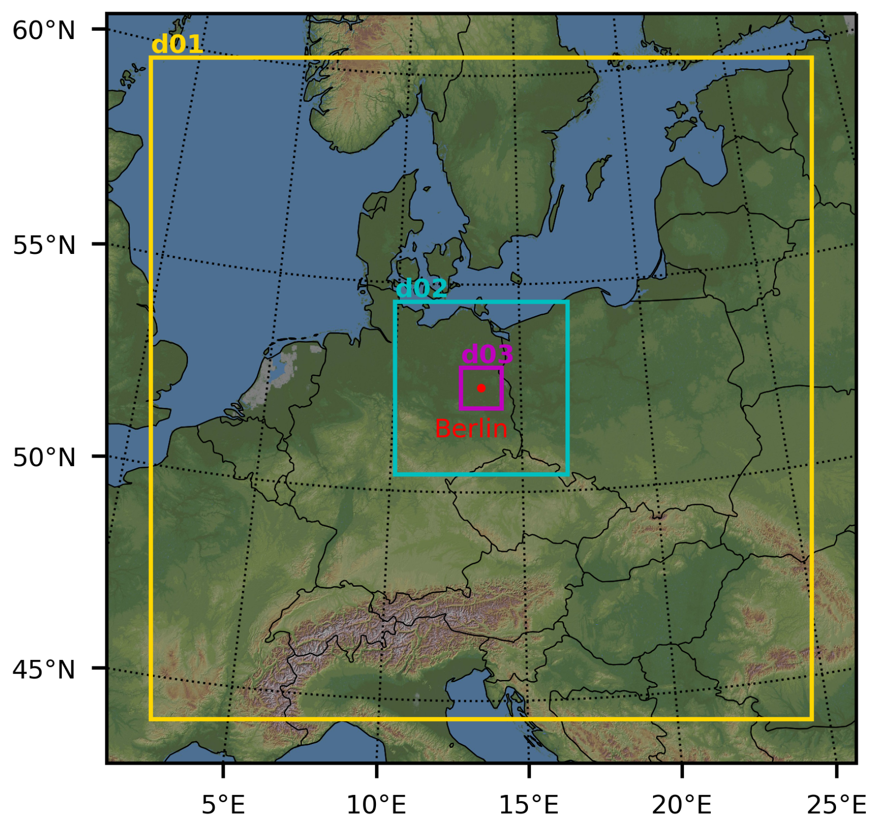
In this study, we present a meso-scale WRF simulation of the urban microclimate in Berlin, Germany. The objective is to derive an accurate estimation of the near-surface urban heat island while also retaining a good station-by-station accuracy (there are four urban and five rural stations). In comparison to previous microclimate studies of Berlin, the manuscript contains several novelties. In particular, (i) the use of the mid-resolution Copernicus Impervious Density data as urban fraction and the Corine Land Cover for the mapping of the urban fractions to the urban categories, (ii) the incorporation of a LUCY-based anthropogenic heat profile in the SLUCM, (iii) the use of high-resolution Berlin City Geography Markup Language (CityGML) data for the estimation of the building height densities required by the MLUCM and, finally, (iv) the comparison of several UHI intensity calculation methods. Section 2 describes the case study and the methodology. Section 3 contains the main simulation results and their discussion. Section 4 presents our conclusions and the future research outlook.

2. Methodology

We used the Weather Research and Forecasting (WRF) model and the WRF Preprocessing System (WPS), both in version 4.2, to generate locally resolved simulation data. The WRF model described by Skamarock et al. [2] is a community atmospheric modeling system that has been used for both atmospheric research and numerical weather prediction (NWP).

2.1. Physical Models

We first performed a preliminary selection of feasible physical models by looking at other similar studies by Jänicke et al. [23], Li et al. [26] and Kuik et al. [43]. To then select the best combination, we performed a small sensitivity study, in which we select an intitial configuration and do 1–2 variations per model type out of our preliminary selection of feasible models. The physical models available in WRF have all been described and referenced by Skamarock et al. [2].
For micro-physics, we mainly used the “WRF single-moment five-class scheme” (WSM5) and compared the results to the “Purdue Lin scheme” (Lin). For cumulus parameterization we used the “Kain Fritsch (new eta) scheme”, but only in the coarsest domain d01. For the planetary boundary layer (PBL), we used the local TKE scheme “Bougeault–Lacarrére” (BouLac) and compared it to the non-local “Yonsei University” (YSU) scheme. According to Skamarock et al. [2], the surface layer (SL) schemes are tied to certain PBL schemes: with the Boulac PBL scheme, we used the “Eta surface layer scheme (MYJ)” and with the YSU PBL scheme, we used the “Revised MM5 surface layer scheme” (RMM5). We also compared the “Noah Multi-Parameterization” (Noah-MP or N-MP) land surface model (LSM) to the classic “Noah” land surface model. For shortwave and longwave radiation, we tested the “Dudhia” (Dud) and “Rapid Radiative Transfer Model” (RRTM) schemes, respectively, and also compared results to using the global parameterization of the RRTM scheme (RRTMG) for both shortwave and longwave radiation. Finally, we tested all of the available urban parameterizations: the basic “Slab” approach, the “Single Layer Urban Canopy Model” (SLUCM) and the “Multilayer Urban Canopy Model” (MLUCM), which consisted of the Building Effect Parameterization (BEP) coupled to the Building Energy Model (BEM). All combinations of physical and urban models tested in this study are shown in Table 1.

2.2. Domain and Boundary Conditions

The simulation domain consisted of a region of 1785 k m × 1785 k m centered on the city of Berlin (13.44° E, 52.51° N). The city of Berlin had a population of 3.5 million inhabitants and covered an area of 892 km2 at the time. The Lambert conformal projection with true latitudes of 52.04° and 52.98°, and a standard longitude of 13.44° was used to define the simulation domain. The domain decomposition was similar to the one by Li et al. [26] with a main domain d01 and two nested domains d02 and d03 to better resolve the urban environment. The domains are shown in Figure 1.
To facilitate inter-study comparison, we simulated the summertime period from 21 June 2010 to 4 July 2010, which was originally selected by Li et al. [25] due to clear sky and calm wind situations. The first day was disregarded in the evaluation as simulation “spin-up” time. The initial conditions and lateral boundary conditions (forcing) were generated with the WPS from GFS analysis data with a resolution of 0.5° and 6 h time intervals [45].
The domain decomposition was based on the work by Li et al. [26], who specified the lateral grid spacing, the parent grid indices and the number of lateral grid points (which are identical for W-E and S-N direction). While the lateral resolution is the same for all models, we had to choose different vertical grids for the different urban models, as the Slab and SLUCM models do not resolve the urban canopy, while the MLUCM does resolve the urban canopy. To define the vertical resolution for the Slab and SLUCM models, we specified the first-layer thickness of 50 m and used the automatic stretching of WRF to generate a total of 35 layers up to a top-level pressure of 5000 Pa . For the MLUCM model, we manually specified the 51 η levels defined by Salamanca et al. [41]. These levels led to finer vertical grid sizes with approximate thicknesses of 5 m, 15 m, 25 m, 35 m and 45 m in the first few layers. The parameters specifying the domain decomposition are given in Table 2.

2.3. Land Use/Land Cover

The WRF model used land use/land cover data to categorize urban and rural surface properties. By default, the Moderate Resolution Imaging Spectroradiometer (MODIS) land use data set with 30 s resolution was used. The 17 categories were defined by the International Geosphere–Biosphere Programme (IGBP) and an additional category 21 for lakes was used by WRF. In addition, we implemented the CORINE Land Cover (CLC) data 2012 with 100 m resolution from the European Union’s Earth Observation Programme Copernicus. The CORINE Land Cover data was also used to derive three urban categories for use with the urban models implemented in WRF. A workflow was established using QGIS (with GRASS and GDAL libraries) and custom Python scripts to convert the data to the format needed by WRF. Firstly, we changed the projection from the source coordinate system (EPSG:3035) to the coordinate system used by WRF (EPSG:4326). Secondly, we converted the classification from CORINE Land Cover into MODIS IGBP categories. Finally, we transformed the data from the GeoTiff format into tiled binary files that can be read by WRF.
The conversion of categories from CORINE to the classification by the United States Geological Survery (USGS) was adapted from Jänicke et al. [23], who modified the original conversion table of Pineda et al. [46]. The conversion from USGS to MODIS IGBP was done according to the WRF model documentation [47]. The resulting reclassification from CORINE Land Cover to MODIS IGBP (including lakes and urban categories) is presented in Table 3. In the urbanized WRF simulations with the SLUCM or MLUCM, the urban categories 31 to 33 allowed a more detailed description of the urban morphology. In the Slab model, only the single urban category 13 was used.
As the CLC data only covered countries of the European Union, we used WRF’s capability to blend different data sets. This way, the default MODIS data set was used where the higher resolved CLC data was not available. The resulting land use data of the main domain d01 and the nested domains d02 and d03 is shown in Figure 2.
For one of our evaluation methods to determine the UHI intensity, which is described in Section 3.2, we used a virtual rural reference simulation. In this hypthetical scenario, the urban area was replaced by a fictitious rural area. Therefore, in the original CORINE landcover dataset, all urban categories were replaced by rural categories as follows: Urban category 31 was remapped to rural category 12, category 32 was remapped to category 5 and category 33 was remapped to category 1. The resulting land use map of the virtual rural reference simulation in domain d03 is also shown in Figure 2.

2.4. Urban Morphology

The accuracy of the urban models additionally depends on the urban morphology of the city. While in the Slab model the urban morphology was not included, the UCM models needed several parameters: both the SLUCM and MLUCM needed the mean urban fraction λ U , the mean building width l ¯ and the mean road width w ¯ . The SLUCM model also used the mean building height H ¯ and its standard deviation σ H . The MLUCM model, however, used a more detailed statistical representation of building heights: the probability γ H that a building with a certain height occurs. The urban morphology parameters are presented in Table 4.
To implement the detailed urban fraction map into the WRF model, we used the Copernicus Impervious Density (IMD) 2015 data with 100 m × 100 m resolution. On the one hand, this data was interpolated by WRF onto the grid tiles and used in the UCM simulations. On the other hand, we derived the median urban fraction λ U for each of the three urban classes of the CLC 2012 dataset within the region of the city of Berlin.
To calculate the mean building heights H ¯ and their standard deviations σ H , which were needed for the SLUCM, we used the CityGML data of Berlin rastered to a digital surface model (DSM) with a resolution of 1 m × 1 m . This data was originally generated during the study of Heldens et al. [48]. An alternative was the coarser resolved Copernicus Urban Atlas Building Height 2012 (DHM2012) data with 100 m × 100 m resolution, which led to similar results in preliminary tests. To obtain the statistical representation of building heights γ H for the MLUCM model, the building heights were separated into several bins and the fraction of the occurrence of each bin was counted. We evaluated heights in the range from 2.5 m to 37.5 m and separated them into 7 bins of 5 m width. Values smaller than the lower bound of 2.5 m were discarded, but values larger than the upper bound of 37.5 m were included in the last bin. The bins were then representative of the heights 5, 10, 15, 20, 25, 30 and 35 m .
To obtain the mean building widths l ¯ and mean street widths w ¯ , we ran the Morphometric Calculator from the Urban Multi-scale Environmental Predictor (UMEP) by Lindberg et al. [49] as plugin in QGIS 3. This tool also used the rastered CityGML data of Berlin by Heldens et al. [48] as a DSM. In the setup of the UMEP Morphometric Calculator, we set the wind direction search interval to 15 deg. From the output, we only evaluated the isotropic results, which were calculated by UMEP by integrating the results of all wind directions. The Morphometric Calculator needed a user specified vector grid. We tested three different grids with different resolutions and selected the medium grid with 250 m × 250 m tiles. We only regarded the grid tiles that were inside the city boundary of Berlin. Finally we disaggregated the grid into the three urban categories specified by CLC and kept only tiles, which were fully occupied by DSM data of the currently investigated urban category. From the output, we used the plan area index λ P and the frontal area index λ F to approximate the mean building widths l ¯ and road widths w ¯ on the basis of the equations introduced by Kanda et al. [50] in the form given by Afshari and Ramirez [51]:
l ¯ = H ¯ · λ P λ F w ¯ = l ¯ · ( 1 λ P 1 ) .
In addition to the urban morphology parameters, urbanized WRF simulations (using the SLUCM or MLUCM) needed several building properties. While these properties could be specified for each category, the values we found in the literature were independent of the urban category. The urbanized WRF setup included default values that we partially adjusted to more realistic values for the city of Berlin. The values we believed to be important are given in Table 5.

2.5. Anthropogenic Heat

To estimate the anthropogenic heat generated in the city, we ran the LUCY QF model from the UMEP plugin for QGIS. The methodology of the model was described by Allen et al. [17]. The resulting values of anthropogenic heat were used in the SLUCM model.
The LUCY QF model needed the mean daily temperatures for the investigated time period specified in Section 2.2. We chose to take the mean value of the temperature measurements from the four urban stations operated by the Deutsche Wetterdienst (DWD) listed in Table 9. We averaged the hourly values to obtain daily values for the simulation period regarded in this work. To spatially disaggregate the anthropogenic heat by population, the model needed the absolute population on a vector grid in shapefile format. We defined a grid with 100 m by 100 m resolution and used the population values from the Urban Atlas 2012 dataset. To scale this data to the desired vector grid, we first calculated the population density per 10,000 m2 for every shape in the original Urban Atlas data. Then, we rastered the shapes to the target grid of 100 m by 100 m resolution, which resulted in the total population per grid tile. The LUCY model also needed several parameters from a namelist file, where we retained the default values. Finally, the LUCY model read further values from a global national energy use database, in which we updated the default values for Germany by publicly available energy use data for the year 2010. The updated values are listed in Table 6.
The LUCY model calculated the anthropogenic heat flux Q separated into three sources (buildings, motorized traffic and metabolism). The model produced results for every hour of the investigated period and every grid tile. We used the spatial resolution to aggregate the anthropogenic heat flux into the three different urban categories specified by CLC. Then we calculated daily profiles of the mean anthropogenic heat flux Q ¯ for each category. To prepare the data for the WRF model, we calculated the maximum values of total anthropogenic heat Q ¯ max for each category, see Table 7. However, the LUCY model calculated the total anthropogenic heat flux Q for the whole area of the provided grid tiles and, during the simulation, WRF would multiply these values by the urban fraction of the grid tile. Hence, WRF would actually interpret the values as anthropogenic heat per urban area. For this reason, we divided the anthropogenic heat by the values of urban fraction given in Table 4 to obtain the anthropogenic heat per urban area Q / λ U . However, we noticed that the value for category 33 was unexpectedly low. The explanation for that was that the LUCY model scaled the anthropogenic heat mainly based on population data. The population data was based on the number of registered inhabitants, which was understandably low in urban areas categorized as commercial, industrial or transporation. To obtain a better representation, we would actually need the average number of people habitually occupying each given urban region, but these numbers were not available. Consequently, we decided to use the mean value for all urban categories, which is also provided in Table 7.
Using the maximum values, a normalized mean profile Q ¯ / Q ¯ max was created. The normalized anthropogenic heat Q ¯ / Q ¯ max is shown in Figure 3 and the numerical values used in WRF are given in Table 8.
In the MLUCM model, only the building anthropogenic heat was considered—which was also seen as dominant in the LUCY estimation method used above for SLUCM. However, this anthropogenic heat in MLUCM was calculated by a dynamic building energy model (BEM). Among the BEM parameters, we mostly retained the default values—with the exception of the fraction of buildings equipped with airconditioning systems which were taken from a study by the German Umweltbundesamt [53]. According to this study, approximately 1% to 2% of the residential buildings and 50% of commercial and administrative buildings were equipped with A/C systems. We adopted these values for setting the “building A/C fraction” for the three different categories in the BEM model: 1% for category 31, 2% for category 32 and 50% for category 33.

3. Results and Discussion

We focused on two different investigations: (i) the first step was an assessment of the sensitivity of model accuracy to variations of physical and urban parameterizations, which led us to select the combination that produces the most accurate estimation of the UHI intensity; (ii) the second step was a comparison of different UHI intensity evaluation methods.

3.1. Sensitivity Analysis

To evaluate model accuracy, we used data for the period of interest from nine meteorological monitoring stations operated by Deutscher Wetterdienst (DWD) [54] in hourly resolution. We evaluated temperature measurements at 2 m height ( T 2   m ) from four urban and four rural stations, and wind speed measurements at 10 m height ( U 10   m ) from two urban and two rural stations. Our selection of DWD stations is compiled in Table 9.
To compare the WRF model to DWD measurement data, we used the Mean Bias Error (MBE) and the Root Mean Square Error (RMSE) as error metrics:
M B E = 1 N i = 1 N y WRF ( t i ) y DWD ( t i ) R M S E = 1 N i = 1 N y WRF ( t i ) y DWD ( t i ) 2 .
To evaluate the performance of different physical and urban parameterizations, we tested several feasible combinations. The WRF simulation results were evaluated at the nine locations of the monitoring stations given in Table 9 and compared to their measurements. The evaluation period starts after the first day has passed at 22 June 2010 00:00 UTC, since the first day was regarded as spin-up period.
We tested several combinations of physical parameterization schemes by varying the microphysics (M-P) scheme, the planetary boundary layer (PBL) and associated surface layer (SL) schemes, the land surface model (LSM), and the shortwave (SW) and longwave (LW) radiation schemes. For this initial sensitivity analysis, the urban canopy was parameterized using the SLUCM model. The resulting error metrics for the different combinations are shown for T 2   m and U 10   m in Table 10. On the one hand, we calculated the RMSE including all measurement stations as a primary metric. On the other hand, we calculated the MBE separately for urban and rural stations to see if there is a difference in bias between simulating urban and rural regions, because such a bias would wrongly increase the UHI intensity.
Based on the results of this first stage, we decided to retain the combination “P1” in Table 10, because this combination led to the lowest overall RMSE and acceptable MBE for urban and rural DWD stations. In the next stage, we analyzed different urban schemes, i.e., the slab model, the single-layer urban canopy model (SLUCM) and the multilayer urban canopy model (MLUCM), which consisted of the Building Effect Parameterization (BEP) coupled to the Building Energy Model (BEM). It should be noted that the results for the urban parameterizations may differ using a different combination of physical schemes. These results correspond to a predominantly dry and low-wind period. The error metrics for the different urban options are shown in Table 11. Within the city, the T 2   m results are best overall for the slab scheme while all three UCMs underestimate U 10   m . It should be noted that in the multi-layer UCM case, the modeled wind speed actually corresponds to the lowest layer, i.e., in our case, the 5 m layer. That explains, to some extent, its higher RMSE when compared to measurements at 10 m . For comparison, Li et al. [26] obtained an overall average RMSE of 1.76 K in their simulation of T 2   m for Berlin. Despite its slight under-performance in T 2   m estimations, the MLUCM performs better than the other schemes when it comes to estimating the UHI intensity, as will be shown in the following.
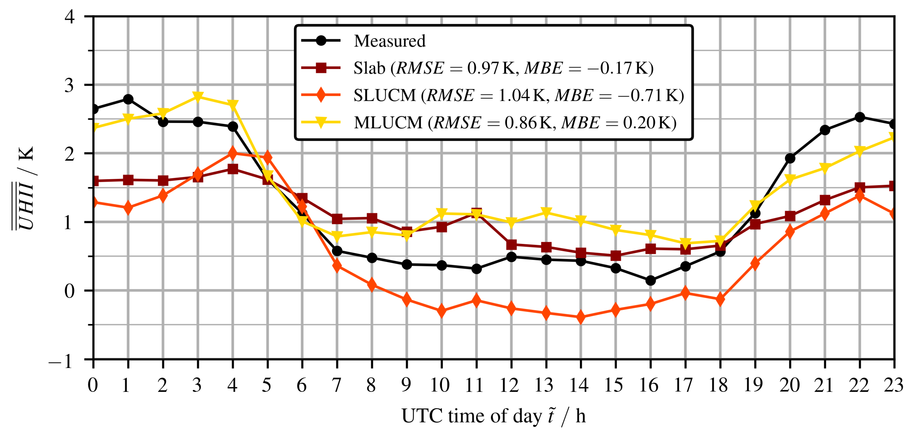
Since our main focus lies on the UHI, we evaluated the model’s ability to predict the UHI intensity variation over an average day. This was done by comparing results from the three urban models to measurements of the DWD monitoring stations. In this analysis, the UHI intensity was assumed to be equal to the difference between the urban T 2   m (taken as the average of the 4 urban stations) and the rural T 2   m (taken as the average of the four rural stations). This corresponds to the “cardinal rural reference” method described in the next section. Equation (6) was used to calculate the UHI intensity profile for an average day, which is shown in Figure 4. The values of MBE and RMSE provided in the Figure, however, are calculated for the entire simulation period and not only for the average day.
With respect to the UHI intensity profile of an average day, the MLUCM model showed the best model/measurement agreement with an RMSE of 0.86 K and an MBE of 0.20 K . The MLUCM also showed a superior qualitative agreement with a significant change from diurnal to nocturnal UHI intensity values. For these reasons, and although the MLUCM slightly underperformed in the error metrics shown in Table 11, we selected this model for the UHI evaluation analysis to be performed in Section 3.2.
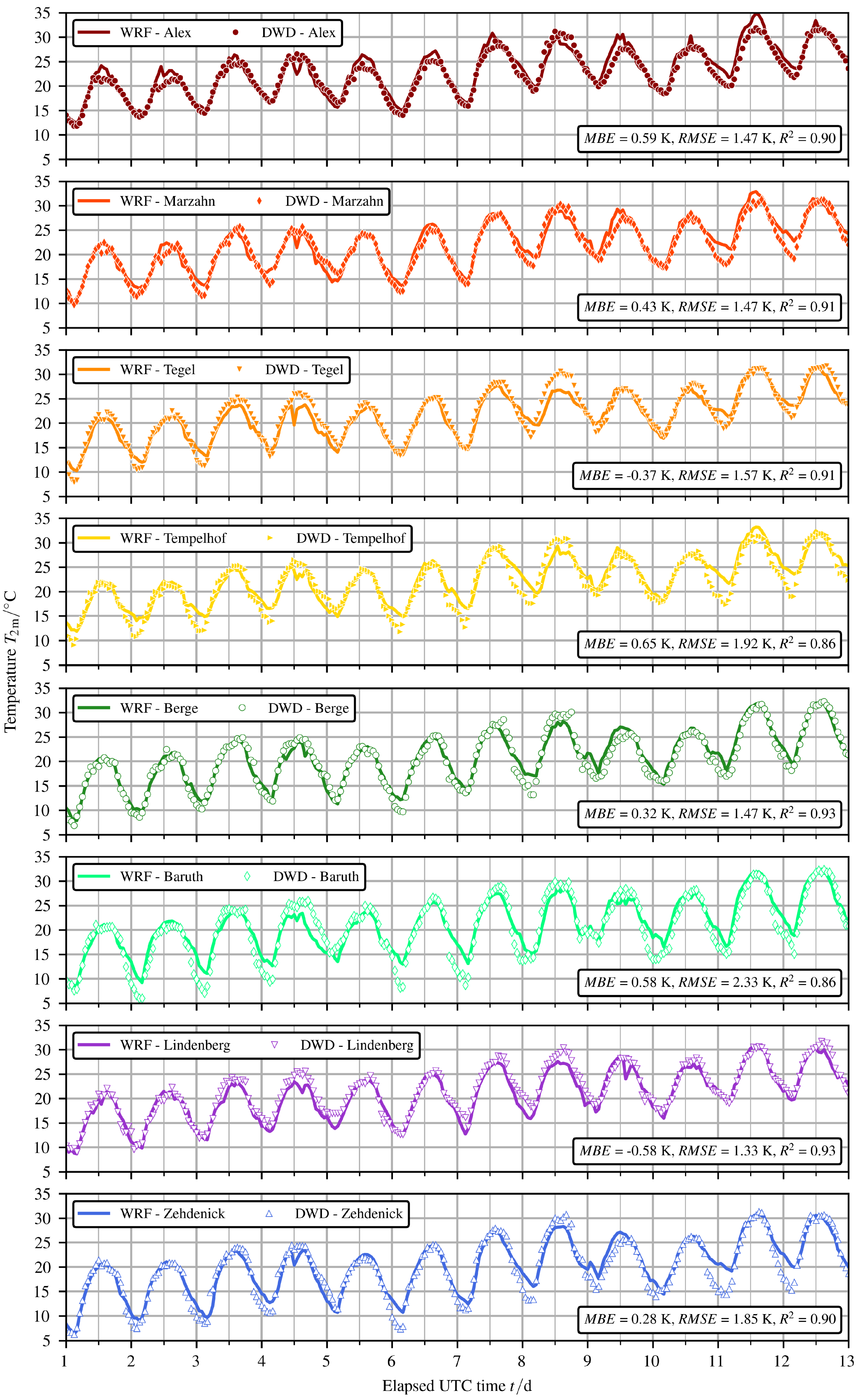
In order to demonstrate the accuracy of the selected UCM for each individual station, the simulated T 2   m values were evaluated at the probe locations of the four urban DWD measurement stations (Alexanderplatz, Marzahn, Tegel and Tempelhof) and the four rural DWD measurement stations (Berge, Baruth, Lindenberg and Zehdenick). The comparison of T 2   m for all stations is shown in Figure 5.
Finally, we want to illustrate the spatial variation of temporally averaged temperatures and wind speeds in the nested domains d02 and d03. The average T 2   m using colored contours and the average U 10   m using velocity vectors are shown in Figure 6. Omitting the first day, a total of 12 days of simulation time were averaged.
We observed higher temperatures in the city of Berlin compared to the immediate surrounding and a predominant north-easterly wind. We would expect the warmer urban air to be advected downstream. Indeed, in d03 the temperatures seem to be elevated downstream of the city. However, if we take a look at d02, we can also see elevated temperatures in a large region south-west of the city well beyond d03, which seems to be rather a synoptic weather pattern than an urban influence. Therefore, special care has to be taken regarding the selection of a rural reference method for UHI intensity evaluation.

3.2. UHI Intensity Evaluation

In order to compare different UHI intensity evaluation methods, we proceeded with a lapse rate correction: temperatures were adjusted to a reference elevation of 56 m above sea level. This corresponds to the mean elevation of all T 2   m probes at the eight urban and rural DWD stations. A dry adiabatic lapse rate of −9.8 × 10⁻³ K m−1 was used.
To assess the UHI intensity, we tested four different methods, among which the first two (described further down) are well known: comparing T 2   m at specific urban and rural locations corresponding to existing monitoring stations. In the third method, herein referred to as the “ring rural reference” method, the rural reference is the spatially averaged T 2   m temperature within a ring surrounding the city and having the same area as the city. In the fourth method, herein referred to as the “virtual rural reference” method, the rural reference is calculated from a fictitious simulation, in which the urban surfaces were replaced with a type of vegetation that is similar to the surrounding rural area. This means that, in contrast with methods 1 and 2, the estimation of the UHI intensity according to methods 3 and 4 cannot be directly compared to measurements, either because it is impractical to measure the average T 2   m temperature of a large ring (method 3) or because the rural reference area does not actually exist and corresponds to a hypothetical scenario (method 4).
Hereafter, T urban refers to T 2   m at selected urban tiles while T rural refers to T 2   m at selected rural tiles. The selection of urban and rural tiles to be considered depends on the rural reference methods that are described below and summarized in Table 12. The spatial average of the UHI intensity is ( · represents a spatial averaging):
U H I I ( t ) = T urban ( t ) T rural ( t ) .
According to the first method, herein referred to as the “cardinal rural reference” (CRR) method, the rural probe locations to be averaged must be approximately in the four cardinal directions relative to the urban area. In our case, the urban probe locations used in the calculation of T urban correspond to the 4 DWD urban stations: Alexanderplatz, Marzahn, Tegel and Tempelhof. The four rural probe locations used in the calculation of T rural correspond to the 4 DWD rural stations: Baruth, Berge, Zehdenick and Lindenberg.
In the second method, herein referred to as the “upstream rural reference” (URR) method, T urban corresponds to one representative urban reference location and T rural corresponds to one upwind rural reference location. In our case, we used the DWD station Alexanderplatz as the urban reference location and the DWD station Zehdenick as the rural reference location.
According to the third method, the “ring rural reference” (RRR) method, the reference rural tiles used for calculating T rural correspond to a ring surrounding the city perimeter, while T urban is calculated using all urban tiles within the city perimeter. The ring was specified as follows: the inner radius of the ring was 26 k m and the ring thickness was 3.765 k m 
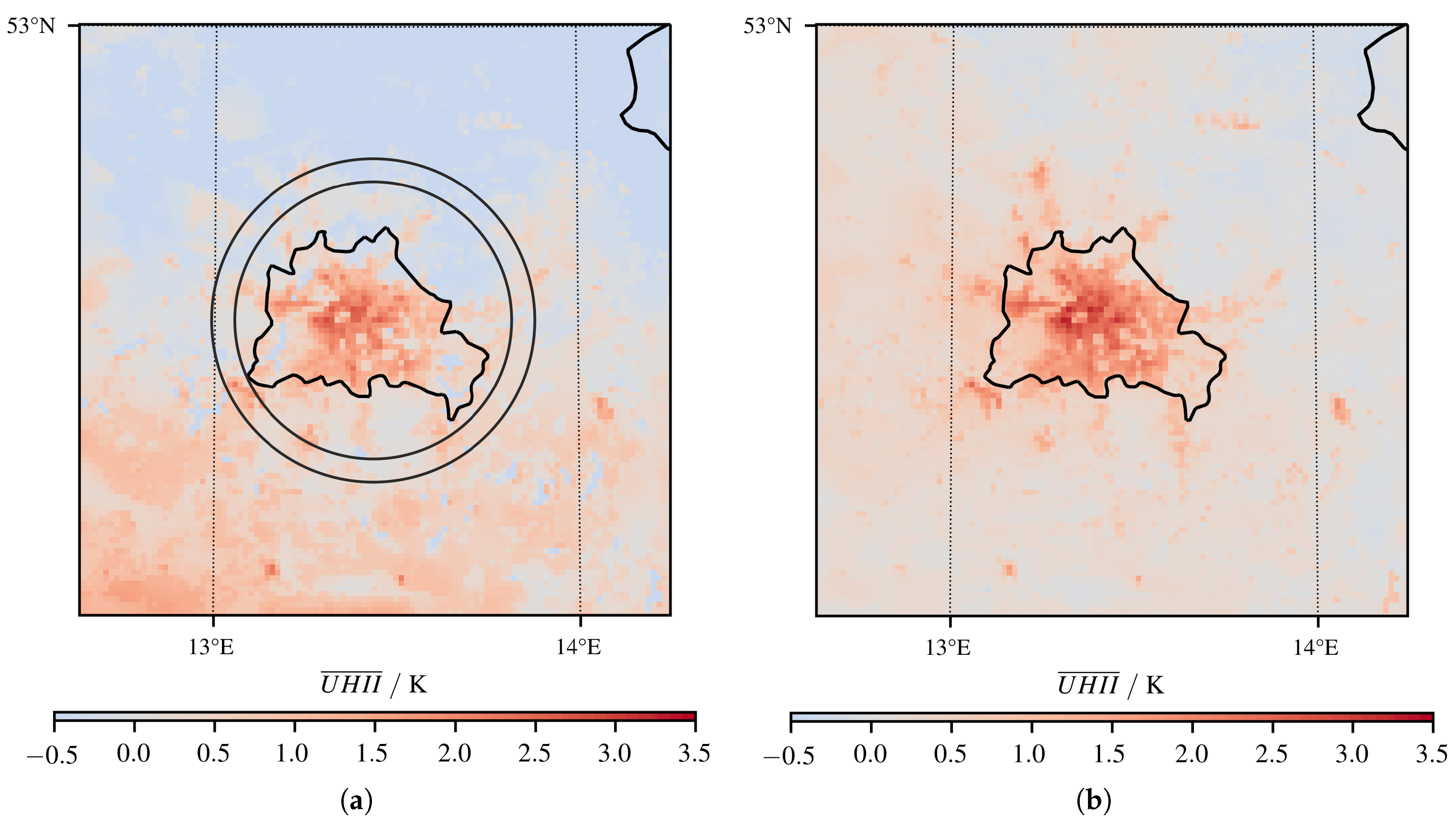
. This way, the ring included 565 tiles, which was the same as the number of urban tiles within the city limits. While the spatially averaged UHI intensity may be calculated according to Equation (3), in order to represent the UHI intensity for each grid tile in a 2D map, we have to use the following equation:
U H I I ( t ) = T urban ( t ) T rural ( t )
According to the RRR method we display U H I I ¯ , which is the time-averaged value of U H I I ( t ) from Equation (4), in Figure 7a.
For the fourth method, the “virtual rural reference” (VRR) method, we compared our base simulation to an alternative simulation corresponding to a hypothetical scenario, where the urban area was replaced by a fictitious rural area, using the modified land-use dataset described in Section 2.3. In this method, we evaluated only the 565 urban tiles located within the city limits for both the base and the hypothetical scenarios. T urban was calculated using the urban tiles in the base scenario. T rural was calculated using the fictitious rural tiles from the hypothetical scenario described above. While the spatially averaged UHI intensity may be calculated according to Equation (3), in order to represent the UHII for each grid tile in a 2D map, we used the following equation:
U H I I ( t ) = T urban ( t ) T rural ( t ) .
According to the VRR method we display U H I I ¯ , which is the time-averaged value of U H I I ( t ) from Equation (5), in Figure 7b. Here, we can clearly observe that the UHI intensity is only high in urban areas, while it is low in rural surroundings. Synoptic weather phenomena do not adversely impact the UHII evaluated according to this method, as they are included in the base case as well as in the fictitious rural scenario.
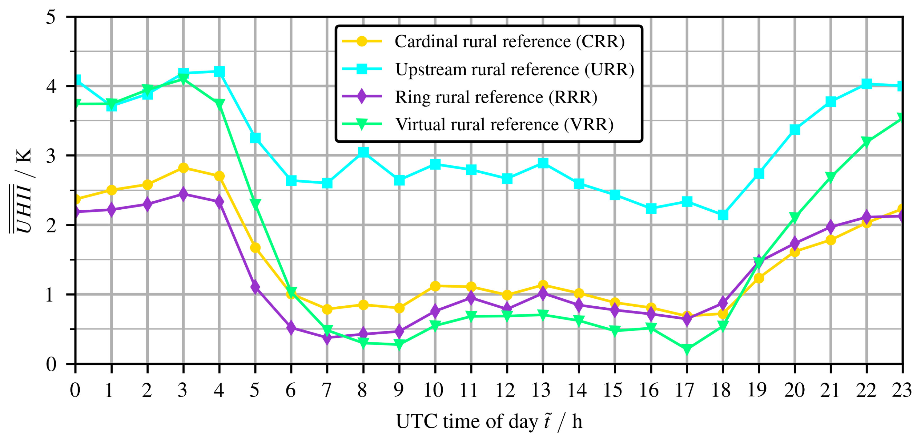
Finally, we compared the UHI intensity profiles for an average day resulting from the four methods described above. These were calculated by averaging the UHI intensity for every hourly time of day t ˜ = 0 , 1 , . . . , 23 over all investigated days N d :
U H I I ¯ ¯ ( t ˜ ) = 1 N d i = 1 N d T urban ( t ˜ + 24 i ) T rural ( t ˜ + 24 i ) .
The resulting U H I I ¯ ¯ profiles for an average day comparing the 4 methods are shown in Figure 8; Table 12 additionally lists the mean, min and max values.
While the UHI intensity profile produced by the ring (RRR) method is very similar to the one calculated by the cardinal (CRR) method, with an average UHII of 1.30 K for RRR and 1.48 K for CRR, the upstream (URR) method delivered consistenly higher UHI intensity values throughout the day, with a min value exceeding 2 K . The average URR UHI intensity of 3.13 K is the highest among the four approaches. One explanation may be that the urban station Alexanderplatz, having a very high urban density, has an overall higher UHII than the other urban locations. Moreover, the upwind rural station could have been biased by including synoptic weather differences. In the CRR method, both these phenomena are decreased by averaging several urban and rural probes. This averaging effect is even stronger in the RRR method, where many more values are used. However, one advantage of the URR method was that the upstream rural probe was not biased by the downstream advection of the elevated urban temperatures. Finally, the virtual rural (VRR) method produced intermediate values, nocturnal results similar to the URR method and diurnal results similar to the CRR (or RRR) method. The average VRR UHII is 1.73 K . We believe that the VRR method is superior to the other methods, as it removed the bias created by synoptic weather impact and also benefitted from a strong averaging effect. Furthermore, conceptually, it corresponds more closely to the theoretical definition of the urban heat island (i.e., the idea of the ‘urban increment’ in comparison to a pre-urban situation).
In order to assess whether the selected VRR rural cover appropriately represents the actual rural cover observed in the area immediately surrounding the city, we looked more closely at the results of VRR simulation, i.e., the simulation performed after replacing urban land cover with rural land cover. Specifically, we calculated the overall average T 2   m temperature within the city as well as within the ring (defined previously for the RRR method). Similarly, we calculated the standard deviation σ T 2   m of the spatial dispersion of both temperature values in their respective regions of analysis. The results are 20.15 ± 0.62 °C for the virtual rural region and 20.41 ± 0.44 °C for the actual rural region (ring). This indicates that temperature and standard deviation in the two regions are close. Of course, this can be improved since the virtual rural region’s average temperature is slightly lower and its dispersion slightly higher. Future research is required to find an optimal approach to populating the city with the most representative rural land cover in the VRR method.
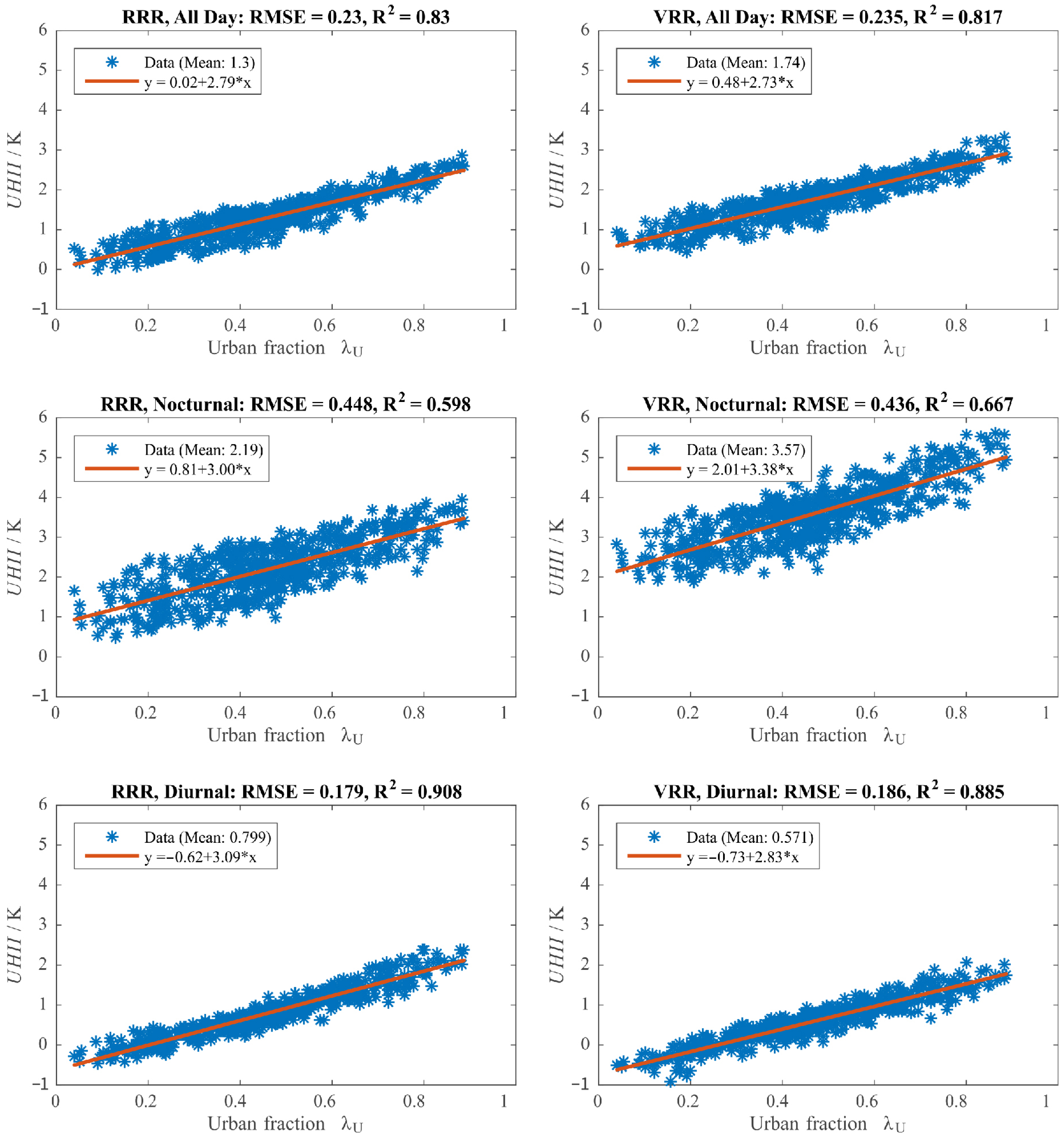
Finally, we studied the dependence of the average UHI intensity on the urban fraction (in the urban region) for the RRR and VRR methods. We estimated linear regression fits for different time periods. The results are shown in Figure 9. The first row corresponds to the overall average UHII (‘All Day’), while the second and third rows correspond to night-time (‘Nocturnal’) and day-time (‘Diurnal’) averages. The fit of the overall average UHII is quite good for both RRR and VRR methods with R 2 values exceeding 0.80. The intercept value of the fitted regression line is almost zero for RRR. This means that tiles with zero urban fraction (e.g., parks) located within the city are expected to have negligible UHII. On the other hand, the intercept value of the fitted regression line is close to 0.5 K for VRR. So, according to this method, there is a residual UHII within the city, even in tiles with zero urban fraction. It seems reasonable to assume that the residual UHII for fully vegetated urban tiles cannot be nil since they are surrounded by, or adjacent to, tiles with non-zero urban fraction displaying a clearly positive UHII. This result speaks in favor of the VRR method. Interestingly, the slopes of both lines are almost the same, meaning that, despite the differing baseline (intercept) values, the rate of increase of UHII with the urban fraction is similar in both cases. Looking at the nigh-time data points (second row of plots), it is obvious that there is much more dispersion around the regression line, for both methods. However, the VRR method results in a better fit: R 2 = 0.677 instead of R 2 = 0.598 . The RMSE is also smaller in the VRR method. The generally higher dispersion of data points around the regression line is indicative of the fact that the urban fraction alone does not fully explain the nocturnal UHI. There are other parameters that should be included in the fit. For instance, the rate of nocturnal long-wave radiative release of urban heat is highly dependent on the sky view factor (more so than the diurnal short-wave radiative heat gain); in other words, the actual 3D configuration of the built-up area matters more at night [55,56]. This contrasts with the diurnal regression (third row of plots) where the dispersion is small and the R 2 is high, indicating that the urban fraction is the predominant explanatory factor.

4. Conclusions

We presented a meso-scale simulation of the urban microclimate in Berlin during the summer period 21 June 2010 to 4 July 2010. The objective of our study was to derive an accurate estimate of the UHI intensity. We compared different physical schemes, different urban canopy schemes and different methods for estimating the UHI intensity. The urban fraction of each urban category was derived using the Copernicus Impervious Density data and the CORINE Land Cover data. High-resolution CityGML data was used to estimate the building height densities required by the MLUCM. Within the SLUCM, a LUCY-based anthropogenic heat profile was implemented. The optimal model configuration was found to be a combination of the WSM5 microphysics scheme, the Bougeault-Lacarrère planetary boundary layer scheme, the eta similarity (MYJ) surface layer scheme, the Noah-MP land surface model, the Dudhia/RRTM radiation schemes and the MLUCM (BEP + BEM). Our UHI intensity results agreed well with measurements (root mean squared error of 0.86 K and mean bias error of 0.20 K ).
We compared several UHI intensity calculation methods: the “cardinal rural reference” (CRR) method, the “upstream rural reference” (URR) method, the “ring rural reference” (RRR) method and the “virtual rural reference” (VRR) method. The URR method delivered consistently higher UHI intensity values throughout the day while the CRR and RRR methods were biased by the downstream advection of the elevated urban temperatures. We concluded the superiority of the VRR method, as it removed the bias created by synoptic weather impact and also benefitted from a strong averaging effect. We also analyzed the dependence of UHII on urban fractions for the RRR and VRR methods. The dependence of the overall average UHII on λ U was strong with R 2 values exceeding 0.80 for both linear fits. However, in the RRR case, the linear fit implied a negligible UHII in urban tiles with zero urban fraction while the VRR case indicated a non-zero residual UHII. We argued that this fact spoke in favor of the VRR method, since the urban tiles with zero urban fraction are bound to be influenced by the positive average UHI of the neighboring tiles with non-zero λ U . Although the choice of the fictitious rural vegetation type is, necessarily, somewhat arbitrary, we showed that the near-surface air temperature and the standard deviation of its spatial dispersion calculated within the city as well as within the ring (defined for the RRR method) are close.
Suggested future research tracks include (i) optimal approach to populating the city with the most representative rural land cover in the VRR method, (ii) extension of the sensitivity analysis to urban morphology and building parameters to better understand their impact on UHI intensity, (iii) inclusion of locational urban explanatory factors other than the urban fraction (for instance, building height, the ratio of building height over street width, proximity to the city center, average wind speed, average air humidity, water surface area, etc.) in the regression of average UHII, (iv) improvement of the LUCY anthropogenic heat flux estimate for the commercial/industrial urban category and (v) a more accurate estimation of the soil moisture initial conditions.

Author Contributions

Conceptualization, A.A.; methodology, J.V. and A.A.; software, J.V.; validation, J.V. and A.A.; formal analysis, J.V.; investigation, J.V.; writing—original draft preparation, J.V. and A.A.; writing—review and editing, J.V. and A.A.; visualization, J.V.; supervision, A.A.; project administration, A.A.; funding acquisition, A.A. All authors have read and agreed to the published version of the manuscript.

Funding

This research was supported by the Fraunhofer Internal Programs under Grant No. Attract 003-695033.

Acknowledgments

The authors acknowledge the support of Sebastian Stadler in preparing the WRF input datasets and the support of Alberto Martilli and Fei Chen in the configuration of the urban canopy schemes. The authors acknowledge the use of imagery from the NASA Worldview application (https://worldview.earthdata.nasa.gov), part of the NASA Earth Observing System Data and Information System (EOSDIS).

Conflicts of Interest

The authors declare no conflict of interest. The funders had no role in the design of the study; in the collection, analyses, or interpretation of data; in the writing of the manuscript, or in the decision to publish the results.

Abbreviations

The following abbreviations are used in this manuscript:
BEMBuilding Energy Model
BEPBuilding Environment Parameterization
BouLacBougeault–Lacarrére
BUBBLEBasel Urban Boundary Layer Experiment
CORINECoordination of Information on the Environment
COSMOConsortium for Small-Scale Modeling
CRRCardinal Rural Reference
DCEPDouble Canyon Effect Parametrization
DWDDeutscher Wetterdienst
EPSGEuropean Petroleum Survey Group Geodesy
GISGeographic Information System
IEAInternational Energy Agency
IGBPInternational Geosphere-Biosphere Programme
LCZLocal Climate Zones
LSMLand Surface Model
LUCYLarge Scale Urban Consumption of Energy
MLUCMMulti-Layer UCM
M-PMicrophysics
MYJMellor-Yamada-Janjić
Noah-MP, N-MPNoah Multi-Parameterization
NWPNumerical Weather Prediction
PBLPlanetary Boundary Layer
RRRRing Rural Reference
RRTMRapid Radiative Transfer Model
SLSurface Layer
SLUCMSingle-Layer UCM
UCMUrban Canopy Model
UHIUrban Heat Island
UHIIUrban Heat Island Intensity
URRUpstream Rural Reference
USGSUnited States Geological Survey
USGSUS Geological Survey
VRRVirtual Rural Reference
WPSWRF Preprocessing System
WRFWeather Research and Forecasting
WUDAPTWorld Urban Database and Access Portal Tool
YSUYonsei University

References

  1. Barlow, J.F. Progress in observing and modelling the urban boundary layer. Urban Clim. 2014, 10, 216–240. [Google Scholar] [CrossRef] [Green Version]
  2. Skamarock, W.C.; Klemp, J.B.; Dudhia, J.; Gill, D.O.; Liu, Z.; Berner, J.; Wang, W.; Powers, J.G.; Duda, M.G.; Barker, D.; et al. A Description of the Advanced Research WRF Model Version 4; Technical Report NCAR/TN-556+STR; UCAR/NCAR: Boulder, CO, USA, 2019. [Google Scholar] [CrossRef]
  3. Baldauf, M.; Seifert, A.; Förstner, J.; Majewski, D.; Raschendorfer, M.; Reinhardt, T. Operational Convective-Scale Numerical Weather Prediction with the COSMO Model: Description and Sensitivities. Mon. Weather Rev. 2011, 139, 3887–3905. [Google Scholar] [CrossRef]
  4. Liu, Y.; Chen, F.; Warner, T.; Basara, J. Verification of a Mesoscale Data-Assimilation and Forecasting System for the Oklahoma City Area during the Joint Urban 2003 Field Project. J. Appl. Meteorol. Climatol. 2006, 45, 912–929. [Google Scholar] [CrossRef]
  5. Taha, H. Modifying a Mesoscale Meteorological Model to Better Incorporate Urban Heat Storage: A Bulk-Parameterization Approach. J. Appl. Meteorol. 1999, 38, 466–473. [Google Scholar] [CrossRef]
  6. Masson, V. Urban surface modeling and the meso-scale impact of cities. Theor. Appl. Climatol. 2006, 84, 35–45. [Google Scholar] [CrossRef]
  7. Best, M.J. Representing urban areas within operational numerical weather prediction models. Bound. Layer Meteorol. 2005, 114, 91–109. [Google Scholar] [CrossRef]
  8. Grimmond, C.S.B.; Blackett, M.; Best, M.J.; Barlow, J.; Baik, J.J.; Belcher, S.E.; Bohnenstengel, S.I.; Calmet, I.; Chen, F.; Dandou, A.; et al. The International Urban Energy Balance Models Comparison Project: First Results from Phase 1. J. Appl. Meteorol. Climatol. 2010, 49, 1268–1292. [Google Scholar] [CrossRef]
  9. Grimmond, C.S.B.; Blackett, M.; Best, M.J.; Baik, J.J.; Belcher, S.E.; Beringer, J.; Bohnenstengel, S.I.; Calmet, I.; Chen, F.; Coutts, A.; et al. Initial results from Phase 2 of the international urban energy balance model comparison. Int. J. Climatol. 2011, 31, 244–272. [Google Scholar] [CrossRef] [Green Version]
  10. Masson, V. A Physically-Based Scheme For The Urban Energy Budget In Atmospheric Models. Bound. Layer Meteorol. 2000, 94, 357–397. [Google Scholar] [CrossRef]
  11. Kusaka, H.; Kondo, H.; Kikegawa, Y.; Kimura, F. A Simple Single-Layer Urban Canopy Model For Atmospheric Models: Comparison With Multi-Layer And Slab Models. Bound. Layer Meteorol. 2000, 101, 329–358. [Google Scholar] [CrossRef]
  12. Martilli, A.; Clappier, A.; Rotach, M.W. An Urban Surface Exchange Parameterisation for Mesoscale Models. Bound. Layer Meteorol. 2002, 104, 261–304. [Google Scholar] [CrossRef]
  13. Schubert, S.; Grossman-Clarke, S.; Martilli, A. A Double-Canyon Radiation Scheme for Multi-Layer Urban Canopy Models. Bound. Layer Meteorol. 2012, 145, 439–468. [Google Scholar] [CrossRef]
  14. Salamanca, F.; Martilli, A. A new Building Energy Model coupled with an Urban Canopy Parameterization for urban climate simulations—Part II. Validation with one dimension off-line simulations. Theor. Appl. Climatol. 2010, 99, 345–356. [Google Scholar] [CrossRef]
  15. Jin, L.; Schubert, S.; Fenner, D.; Meier, F.; Schneider, C. Integration of a Building Energy Model in an Urban Climate Model and its Application. Bound. Layer Meteorol. 2020. [Google Scholar] [CrossRef]
  16. Sailor, D.J. A review of methods for estimating anthropogenic heat and moisture emissions in the urban environment. Int. J. Climatol. 2011, 31, 189–199. [Google Scholar] [CrossRef]
  17. Allen, L.; Lindberg, F.; Grimmond, C.S.B. Global to city scale urban anthropogenic heat flux: Model and variability. Int. J. Climatol. 2011, 31, 1990–2005. [Google Scholar] [CrossRef]
  18. Salamanca, F.; Georgescu, M.; Mahalov, A.; Moustaoui, M. Summertime Response of Temperature and Cooling Energy Demand to Urban Expansion in a Semiarid Environment. J. Appl. Meteorol. Climatol. 2015, 54, 1756–1772. [Google Scholar] [CrossRef]
  19. Oke, T.R.; Mills, G.; Christen, A.; Voogt, J.A. Urban Climates; Cambridge University Press: Cambridge, UK, 2017. [Google Scholar] [CrossRef] [Green Version]
  20. Salamanca, F.; Martilli, A.; Tewari, M.; Chen, F. A Study of the Urban Boundary Layer Using Different Urban Parameterizations and High-Resolution Urban Canopy Parameters with WRF. J. Appl. Meteorol. Climatol. 2011, 50, 1107–1128. [Google Scholar] [CrossRef]
  21. Bohnenstengel, S.I.; Evans, S.; Clark, P.A.; Belcher, S. Simulations of the London urban heat island. Q. J. R. Meteorol. Soc. 2011, 137, 1625–1640. [Google Scholar] [CrossRef]
  22. Wyngaard, J.C. Toward Numerical Modeling in the “Terra Incognita”. J. Atmos. Sci. 2004, 61, 1816–1826. [Google Scholar] [CrossRef]
  23. Jänicke, B.; Meier, F.; Fenner, D.; Fehrenbach, U.; Holtmann, A.; Scherer, D. Urban-rural differences in near-surface air temperature as resolved by the Central Europe Refined analysis (CER): Sensitivity to planetary boundary layer schemes and urban canopy models. Int. J. Climatol. 2017, 37, 2063–2079. [Google Scholar] [CrossRef]
  24. Nemunaitis-Berry, K.L.; Klein, P.M.; Basara, J.B.; Fedorovich, E. Sensitivity of Predictions of the Urban Surface Energy Balance and Heat Island to Variations of Urban Canopy Parameters in Simulations with the WRF Model. J. Appl. Meteorol. Climatol. 2017, 56, 573–595. [Google Scholar] [CrossRef] [Green Version]
  25. Li, H.; Wolter, M.; Wang, X.; Sodoudi, S. Impact of land cover data on the simulation of urban heat island for Berlin using WRF coupled with bulk approach of Noah-LSM. Theor. Appl. Climatol. 2018, 134, 67–81. [Google Scholar] [CrossRef]
  26. Li, H.; Zhou, Y.; Wang, X.; Zhou, X.; Zhang, H.; Sodoudi, S. Quantifying urban heat island intensity and its physical mechanism using WRF/UCM. Sci. Total Environ. 2019, 650, 3110–3119. [Google Scholar] [CrossRef]
  27. Hammerberg, K.; Brousse, O.; Martilli, A.; Mahdavi, A. Implications of employing detailed urban canopy parameters for mesoscale climate modelling: A comparison between WUDAPT and GIS databases over Vienna, Austria. Int. J. Climatol. 2018, 38, e1241–e1257. [Google Scholar] [CrossRef] [Green Version]
  28. Wong, M.M.F.; Fung, J.C.H.; Ching, J.; Yeung, P.P.S.; Tse, J.W.P.; Ren, C.; Wang, R.; Cai, M. Evaluation of uWRF performance and modeling guidance based on WUDAPT and NUDAPT UCP datasets for Hong Kong. Urban Clim. 2019, 28, 100460. [Google Scholar] [CrossRef] [Green Version]
  29. Salamanca, F.; Zhang, Y.; Barlage, M.; Chen, F.; Mahalov, A.; Miao, S. Evaluation of the WRF-Urban Modeling System Coupled to Noah and Noah-MP Land Surface Models Over a Semiarid Urban Environment. J. Geophys. Res. Atmos. 2018, 123, 2387–2408. [Google Scholar] [CrossRef]
  30. Kusaka, H.; Chen, F.; Tewari, M.; Dudhia, J.; Gill, D.O.; Duda, M.G.; Wang, W.; Miya, Y. Numerical Simulation of Urban Heat Island Effect by the WRF Model with 4-km Grid Increment: An Inter-Comparison Study between the Urban Canopy Model and Slab Model. J. Meteorol. Soc. Jpn. Ser. II 2012, 90B, 33–45. [Google Scholar] [CrossRef] [Green Version]
  31. Schubert, S.; Grossman-Clarke, S. Evaluation of the coupled COSMO-CLM/DCEP model with observations from BUBBLE. Q. J. R. Meteorol. Soc. 2014, 140, 2465–2483. [Google Scholar] [CrossRef]
  32. Trusilova, K.; Schubert, S.; Wouters, H.; Früh, B.; Grossman-Clarke, S.; Demuzere, M.; Becker, P. The urban land use in the COSMO-CLM model: A comparison of three parameterizations for Berlin. Meteorol. Z. 2016, 25, 231–244. [Google Scholar] [CrossRef]
  33. Jandaghian, Z.; Berardi, U. Comparing urban canopy models for microclimate simulations in Weather Research and Forecasting Models. Sustain. Cities Soc. 2020, 55, 102025. [Google Scholar] [CrossRef]
  34. Teixeira, J.C.; Fallmann, J.; Carvalho, A.C.; Rocha, A. Surface to boundary layer coupling in the urban area of Lisbon comparing different urban canopy models in WRF. Urban Clim. 2019, 28, 100454. [Google Scholar] [CrossRef]
  35. Loridan, T.; Grimmond, C. Multi-site evaluation of an urban land-surface model: Intra-urban heterogeneity, seasonality and parameter complexity requirements. Q. J. R. Meteorol. Soc. 2012, 138, 1094–1113. [Google Scholar] [CrossRef] [Green Version]
  36. Kusaka, H.; Kimura, F. Coupling a Single-Layer Urban Canopy Model with a Simple Atmospheric Model: Impact on Urban Heat Island Simulation for an Idealized Case. J. Meteorol. Soc. Jpn. Ser. II 2004, 82, 67–80. [Google Scholar] [CrossRef] [Green Version]
  37. Miao, S.; Chen, F.; LeMone, M.A.; Tewari, M.; Li, Q.; Wang, Y. An Observational and Modeling Study of Characteristics of Urban Heat Island and Boundary Layer Structures in Beijing. J. Appl. Meteorol. Climatol. 2009, 48, 484–501. [Google Scholar] [CrossRef]
  38. Schubert, S.; Grossman-Clarke, S. The Influence of green areas and roof albedos on air temperatures during Extreme Heat Events in Berlin, Germany. Meteorol. Z. 2013, 22, 131–143. [Google Scholar] [CrossRef] [Green Version]
  39. Morini, E.; Touchaei, A.; Castellani, B.; Rossi, F.; Cotana, F. The Impact of Albedo Increase to Mitigate the Urban Heat Island in Terni (Italy) Using the WRF Model. Sustainability 2016, 8, 999. [Google Scholar] [CrossRef] [Green Version]
  40. Fallmann, J.; Emeis, S.; Suppan, P. Mitigation of urban heat stress—A modelling case study for the area of Stuttgart. DIE ERDE 2013, 144, 202–216. [Google Scholar]
  41. Salamanca, F.; Martilli, A.; Yagüe, C. A numerical study of the Urban Heat Island over Madrid during the DESIREX (2008) campaign with WRF and an evaluation of simple mitigation strategies. Int. J. Climatol. 2012, 32, 2372–2386. [Google Scholar] [CrossRef]
  42. Jin, L.; Schubert, S.; Salim, M.H.; Schneider, C. Impact of Air Conditioning Systems on the Outdoor Thermal Environment during Summer in Berlin, Germany. Int. J. Environ. Res. Public Health 2020, 17, 4645. [Google Scholar] [CrossRef]
  43. Kuik, F.; Lauer, A.; Churkina, G.; van der Denier Gon, H.A.C.; Fenner, D.; Mar, K.A.; Butler, T.M. Air quality modelling in the Berlin–Brandenburg region using WRF-Chem v3.7.1: Sensitivity to resolution of model grid and input data. Geosci. Model Dev. 2016, 9, 4339–4363. [Google Scholar] [CrossRef] [Green Version]
  44. NASA. NASA Worldview Application, Part of the NASA Earth Observing System Data and Information System (EOSDIS). 2020. Available online: https://worldview.earthdata.nasa.gov (accessed on 9 December 2020).
  45. National Centers for Environmental Prediction. Global Forecast System Analysis Data (GFS-ANL) with 0.5 Degree Resolution. 2020. Available online: https://www.ncei.noaa.gov/data/global-forecast-system/access/grid-004-0.5-degree/analysis/ (accessed on 9 December 2020).
  46. Pineda, N.; Jorba, O.; Jorge, J.; Baldasano, J.M. Using NOAA AVHRR and SPOT VGT data to estimate surface parameters: Application to a mesoscale meteorological model. Int. J. Remote Sens. 2004, 25, 129–143. [Google Scholar] [CrossRef]
  47. NCAR. WRF-ARW Model; NCAR: Boulder, CO, USA, 2019. [Google Scholar] [CrossRef]
  48. Heldens, W.; Burmeister, C.; Kanani-Sühring, F.; Maronga, B.; Pavlik, D.; Sühring, M.; Zeidler, J.; Esch, T. Geospatial input data for the PALM model system 6.0: Model requirements, data sources, and processing. Geosci. Model Dev. Discuss. 2020, 1–62. [Google Scholar] [CrossRef]
  49. Lindberg, F.; Grimmond, C.; Gabey, A.; Huang, B.; Kent, C.W.; Sun, T.; Theeuwes, N.E.; Järvi, L.; Ward, H.C.; Capel-Timms, I.; et al. Urban Multi-scale Environmental Predictor (UMEP): An integrated tool for city-based climate services. Environ. Model. Softw. 2018, 99, 70–87. [Google Scholar] [CrossRef]
  50. Kanda, M.; Kawai, T.; Kanega, M.; Moriwaki, R.; Narita, K.; Hagishima, A. A Simple Energy Balance Model for Regular Building Arrays. Bound. Layer Meteorol. 2005, 116, 423–443. [Google Scholar] [CrossRef]
  51. Afshari, A.; Ramirez, N. Improving the accuracy of simplified urban canopy models for arid regions using site-specific prior information. Urban Clim. 2021, 35, 100722. [Google Scholar] [CrossRef]
  52. Chen, F.; Kusaka, H.; Bornstein, R.; Ching, J.; Grimmond, C.S.B.; Grossman-Clarke, S.; Loridan, T.; Manning, K.W.; Martilli, A.; Miao, S.; et al. The integrated WRF/urban modelling system: Development, evaluation, and applications to urban environmental problems. Int. J. Climatol. 2011, 31, 273–288. [Google Scholar] [CrossRef]
  53. Bettgenhäuser, K.; Boermans, T.; Offermann, M.; Krechting, A.; Becker, D. Klimaschutz durch Reduzierung des Energiebedarfs für Gebäudekühlung; Umweltbundesamt: Dessau-Roßlau, Germany, 2011.
  54. Deutscher Wetterdienst. DWD Open Data-Server Climate Data Center (CDC). 2020. Available online: https://opendata.dwd.de/climate_environment/CDC/ (accessed on 9 December 2020).
  55. Lan, Y.; Zhan, Q. How do urban buildings impact summer air temperature? The effects of building configurations in space and time. Build. Environ. 2017, 125, 88–98. [Google Scholar] [CrossRef]
  56. Chun, B.; Guhathakurta, S. Daytime and nighttime urban heat islands statistical models for Atlanta. Environ. Plan B Urban Anal. City Sci. 2017, 44, 308–327. [Google Scholar] [CrossRef]
Figure 1. Main domain d01 and nested domains d02 and d03. The elevation is illustrated using the “ASTER Global Digital Elevation Map” from Nasa Worldview [44] as background image.
Atmosphere 11 01338 g001
Figure 2. Land use categories using the combined MODIS and CORINE Land Cover (CLC) datasets for the main domain d01 and the nested domains d02 and d03. For the inner domain d03, the modified land use data for the virtual rural reference method is additionally shown, see Section 3.2.
Atmosphere 11 01338 g002
Figure 3. Mean normalized anthropogenic heat profile calculated by the LUCY model. The total value as well as the contributions of buildings, traffic and human metabolism are shown.
Atmosphere 11 01338 g003
Figure 4. Urban heat island (UHI) intensity profiles for an average day comparing the three different urban models to measurements.
Atmosphere 11 01338 g004
Figure 5. Comparison of simulated and measured T 2   m at the probe locations of the four urban DWD measurement stations (Alexanderplatz, Marzahn, Tegel and Tempelhof) and the four rural DWD measurement stations (Berge, Baruth, Lindenberg and Zehdenick).
Atmosphere 11 01338 g005
Figure 6. Average T 2   m contours and U 10   m vectors in the nested domains d02 and d03.
Atmosphere 11 01338 g006
Figure 7. Time-averaged UHI intensity maps for the evaluation methods “ring rural reference” and “virtual rural reference”. (a) Ring rural reference. (b) Virtual rural reference.
Atmosphere 11 01338 g007
Figure 8. Comparison of the UHI intensity profiles of an average day using the four evaluation methods.
Atmosphere 11 01338 g008
Figure 9. Linear regression correlating UHII with urban fraction (left column: RRR, right column: VRR).
Atmosphere 11 01338 g009
Table 1. Combinations of physical and urban parameterizations of Weather Research and Forecasting (WRF) used in this study.
NameM-PPBLSLLSMRadiation SW/LWUrban Model
P1WSM5BouLacMYJN-MPDud/RRTMSLUCM
P2LinBouLacMYJN-MPDud/RRTMSLUCM
P3WSM5YSURMM5N-MPDud/RRTMSLUCM
P4WSM5BouLacMYJNoahDud/RRTMSLUCM
P5WSM5BouLacMYJN-MPRRTMGSLUCM
U1WSM5BouLacMYJN-MPDud/RRTMSlab
U2WSM5BouLacMYJN-MPDud/RRTMSLUCM
U3WSM5BouLacMYJN-MPDud/RRTMMLUCM
Table 2. Discretization parameters to define the three domains d01, d02 and d03. The vertical layers vary for different urban models, as the Slab and single-layer urban canopy model (SLUCM) models do not resolve the urban canopy, while the multi-layer urban canopy model (MLUCM) does resolve the urban canopy.
WRF Parameterd01d02d03
All models
Lateral grid spacing15 km3 km1 km
Starting index in parent grid14560
Number of lateral grid points120156112
Slab/SLUCM
Vertical first layer thickness50 m50 m50 m
Number of vertical grid points353535 
MLUCM
Vertical first layer thickness5 m5 m5 m
Number of vertical grid points515151
Table 3. Reclassification from CORINE land cover to Moderate Resolution Imaging Spectroradiometer (MODIS) International Geosphere–Biosphere Programme (IGBP) including lakes and three urban categories).
IDCORINE Land CoverMODIS IGBPID
1Continuous urban fabricHigh intensity residential32
2Discontinuous urban fabricLow intensity residential31
3–5Industrial/commercial, road and rail networks, port areasCommercial/industrial/transportation33
6AirportsCroplands12
7Mineral extraction sitesBarren or sparsely vegetated16
8,9dump sites, construction sitesCommercial/industrial/transportation33
10,11Green urban areas, sport and leisure facilitiesCropland/natural vegetation mosaic14
12–14Non-irrigated, permanently irrigated land, rice fieldsCroplands12
15–17Vineyards, fruit trees, olive grovesCropland/natural vegetation mosaic14
18PasturesCroplands12
19–22Annual crops, complex cultivation, agriculture, agro forestryCropland/natural vegetation mosaic14
23Broad-leaved forestDeciduous broadleaf forest4
24Coniferous forestEvergreen needleleaf forest1
25Mixed forestMixed forests5
26Natural grasslandsGrasslands10
27–29Moors, sclerophyllous vegetation, transitional woodland-shrubOpen shrublands7
30–33Beaches/dunes/sands, bare rocks, sparsely vegetated, burntBarren or sparsely vegetated16
34Glaciers and perpetual snowSnow and ice15
35–38Inland marshes, peat bogs, salt marshes, salinesPermanent wetlands11
39Intertidal flatsWater17
40–43Water courses, water bodies, coastal lagoons, estuariesLakes21
44Sea and oceanWater17
Table 4. Urban morphology parameters used in the urbanized WRF simulations (SLUCM or MLUCM).
ParameterSymbolUnitValue for Urban Category
313233
SLUCM and MLUCM
Urban fraction λ U %458675
Mean building width l ¯ m13.219.825.2
Mean road width w ¯ m17.612.427.4
SLUCM
Mean building height H ¯ m11.319.912.7
Std. dev. of building heights σ H m7.57.38.3
MLUCM
Building heights 5 m γ H = 5 %37927
Building heights 10 m γ H = 10 %25636
Building heights 15 m γ H = 15 %18817
Building heights 20 m γ H = 20 %144511
Building heights 25 m γ H = 25 %4276
Building heights 30 m γ H = 30 %143
Building heights 35 m γ H = 35 %111
Table 5. Building properties used in the urbanized WRF simulations (SLUCM or MLUCM).
ParameterSymbolValueSource
Thicknesses of the 4 roof and wall layers d r and d w 0.05, 0.05, 0.1, 0.2 mJänicke et al. [23]
Thicknesses of the 4 ground layers d g 0.05, 0.25, 0.50, 0.75 mWRF default
Vol. heat capacity of roof, wall and ground c r , c w and c g 2.3 × 10⁶ J m−3 K−1Jänicke et al. [23]
Thermal conductivity of roof and wall k r and k w 1.54 W m−1 K−1Jänicke et al. [23]
Thermal conductivity of ground k g 0.67 W m−1 K−1Jänicke et al. [23]
Surface albedo of roof and wall α r and α w 0.2Salamanca et al. [20]
Surface albedo of ground α g 0.15Salamanca et al. [20]
Surface emissivity of roof and wall ϵ r and ϵ w 0.9Martilli et al. [12]
Surface emissivity of ground ϵ g 0.95Martilli et al. [12]
Roughness length of roof and ground z 0 , r and z 0 , g 0.01 mChen et al. [52]
Roughness length of wall z 0 , w 0.0001 mChen et al. [52]
Lower boundary temperature for roof and wall T b , r and T b , w 20 °CWRF default
Lower boundary temperature for ground T b , g 10 °CJänicke et al. [23]
Table 6. Values added to the large scale urban consumption of energy (LUCY) database for Germany for the year 2010.
Data EntryValueSource
IEA total final consumption minus transport per year2,043,730 GW hHeadline Energy Data (www.iea.org)
Number of cars owned per 1000 inhabitants516.4Kraftfahrtbundesamt (KBA) Germany
Number of motorcycles owned per 1000 inhabitants46.5Kraftfahrtbundesamt (KBA) Germany
Number of freight vehicles owned per 1000 inhabitants58.0Kraftfahrtbundesamt (KBA) Germany
Total population80,827,000United Nations Population Division
Table 7. Maximum values of total anthropogenic heat emissions disaggregated by urban category.
ParameterUnitCategory 31Category 32Category 33All Cat.
Total anthropogenic heat Q ¯ max (LUCY)W m−224.259.25.5214.0
Total anthropogenic heat per urban area Q ¯ max / λ U W m−253.868.87.446.7
Table 8. Normalized daily profile of total anthropogenic heat emissions from the LUCY model.
ParameterHourly Values
t/h010203040506070809101112131415161718192021222324
Q ¯ / Q ¯ max /%1927405367798994999999100959080726558514336302419
Table 9. Measurement stations used for determining the accuracy of our model setups. The locations of the stations are indicated in the inner nested domain d03 on Figure 2.
Station NameCategoryLocationElevationMeasurement Used
AlexanderplatzUrban13.4057° E, 52.5198° N36 m T 2   m
MarzahnUrban13.5598° E, 52.5447° N60 m T 2   m
TegelUrban13.3088° E, 52.5644° N36 m T 2   m , U 10   m
TempelhofUrban13.4021° E, 52.4675° N48 m T 2   m , U 10   m
BergeRural12.7867° E, 52.6198° N40 m T 2   m
BaruthRural13.4996° E, 52.0614° N55 m T 2   m
LindenbergRural14.1180° E, 52.2085° N98 m T 2   m , U 10   m
MünchebergRural14.1232° E, 52.5176° N63 m U 10   m
ZehdenickRural13.3268° E, 52.9664° N51 m T 2   m
Table 10. Error metrics for temperature T 2   m (in K) and wind speed U 10   m (in m/s) comparing several combinations of physical models. The RMSE was calculated for all measurement stations; the MBE was calculated separately for urban and rural stations.
NamePhysical ModelsVariableRMSEMBE
M-PPBL/SLLSMRad. SW/LWAllUrbanRural
P1WSM5BouLac/MYJN-MPDud/RRTM T 2   m 1.53−0.700.0057
U 10   m 1.13−0.270.096 
P2LinBouLac/MYJN-MPDud/RRTM T 2   m 1.57−0.69−0.04
U 10   m 1.10−0.210.11 
P3WSM5YSU/RMM5N-MPDud/RRTM T 2   m 1.96−1.37−0.63
U 10   m 1.06−0.210.40 
P4WSM5BouLac/MYJNoahDud/RRTM T 2   m 2.15−1.34−1.22
U 10   m 0.99−0.270.05 
P5WSM5BouLac/MYJN-MPRRTMG T 2   m 1.620.381.15
U 10   m 1.15−0.080.27 
Table 11. Error metrics for temperature T 2   m (in K) and wind speed U 10   m (in m/s) comparing the three urban models: Slab, SLUCM and MLUCM (building environment parameterization (BEP)+building energy model (BEM)). The RMSE was calculated for all measurement stations; the MBE was calculated separately for urban and rural stations.
NameUrban ModelVariableRMSEMBE
AllUrbanRural
U1Slab T 2   m 1.49−0.0680.10
U 10   m 1.04−0.460.094 
U2SLUCM T 2   m 1.53−0.700.0057
U 10   m 1.13−0.270.096 
U3MLUCM T 2   m 1.690.280.093
U 10   m 1.23−0.47−0.025
Table 12. The four different evaluation methods and the mean, min and max values of the average day UHI intensity (in K).
MethodEvaluation MethodUHI Intensity
T urban T rural MeanMinMax
CRR4 urban probes4 rural probes1.480.692.82
URR1 urban probe1 upstream rural probe3.132.144.21
RRR565 urban tiles in city565 rural tiles in ring1.300.382.44
VRR565 urban tiles in city565 fictitious rural tiles in city1.740.214.10
Publisher’s Note: MDPI stays neutral with regard to jurisdictional claims in published maps and institutional affiliations.

