Article

Updating Real-World Profiles of Volatile Organic Compounds and Their Reactivity Estimation in Tunnels of Mexico City

by
Violeta Mugica-Álvarez
1,*,
Miguel Magaña-Reyes
2,
Adriana Martínez-Reyes
1,
Jesús Figueroa-Lara
1,
Salvador Blanco-Jiménez
2,
Valia Goytia-Leal
2,
Victor H. Páramo-Figueroa
3 and
Rocío García-Martínez
4
1
Basic Sciences, Universidad Autónoma Metropolitana-Azcapotzalco, Mexico City 02200, Mexico
2
Instituto Nacional de Ecología y Cambio Climático, Mexico City 14210, Mexico
3
Comisión Ambiental de la Megalópolis, Mexico City 11320, Mexico
4
Centro de Ciencias de la Atmósfera, Universidad Nacional Autónoma de México, Mexico City 02202, Mexico
*
Author to whom correspondence should be addressed.
Atmosphere 2020, 11(12), 1339; https://doi.org/10.3390/atmos11121339
Submission received: 31 October 2020 / Revised: 27 November 2020 / Accepted: 2 December 2020 / Published: 9 December 2020
(This article belongs to the Section Air Quality)

Abstract

:
The main objective of this work was to bring to date the exhaust and evaporative volatile organic compound (VOC) profiles from light-duty gasoline vehicles, carrying out a sampling and analysis campaign in two tunnels of Mexico City. The abundance of exhaust-emission VOC profiles was the same in 2018 as in 1998 (alkanes > aromatics > olefins > acetylene), albeit exhibiting large differences (67%, 17%, 12%, and 4% for 2018, and 50%, 26%, 16%, and 8% for 1998, respectively). An important reduction of 69% and 77% in VOC concentrations was registered inside and outside of the tunnel, respectively, in comparison with 1998. In the ambient air, alkanes accounted for 77%, since high concentrations of liquefied petroleum (LP) gas species are still present. Ethylene, propylene, 1-butene, and toluene from tunnel emissions contributed prominently to ozone formation, while the most reactive gasoline vapors were pentenes, pentanes, and butenes, although the ozone formation potential due to VOCs in tunnel emissions and ambient air also had a significant reduction. These results demonstrate that strategies carried out in the last 20 years were successful in achieving a better air quality, although the aromatic and olefin content in gasolines needs to be further reduced to lower the concentrations of toxic and reactive species.

1. Introduction

Volatile organic compounds (VOCs) constitute numerous organic chemicals displaying high vapor pressures under normal temperature conditions. VOCs are emitted from natural and anthropogenic sources such as vehicle exhausts, gasoline and solvent evaporation, industrial processes, and cleaning products, among other sources. Some VOCs have been classified as toxic causing assorted irritation of mucous membranes, eyes, skin, and the respiratory system; furthermore, to make matters worse, they also cause neurobehavioral effects, asthma, cardiovascular illnesses, and various metabolic and malignant diseases, including cancer [1,2,3]. A study in the Mexico City Metropolitan Area (MCMA) reported that a reduction in the annual average concentration of ozone to 0.05 ppm could prevent approximately 400 deaths per year [4]. Additionally, damages to surrounding crops have been documented due to high ozone concentrations [5]. Furthermore, the VOCs and nitrogen oxides (NOx) become precursors of ground-level ozone (O3) upon irradiation by solar light, through photochemical activity in polluted atmospheres.
Tropospheric ozone represents a severe risk to human health [6], as this pollutant is also a radiative forcer that contributes to climate change [7] and causes yield losses in crops at important agricultural regions [8]. The O3 formation rate varies depending on the amount and relative mixing ratios of VOCs and NOx, depicting a nonlinear behavior. Sometimes, O3 production can be controlled by reducing the VOCs (VOC-limited regime) and other times by reducing the NOx emissions (NOx-limited regime) [9]. When ozone formation occurs through the VOC-limited regime, the mechanism involves the formation of the hydroxyl radical (OH) in the atmosphere, which, due to photolysis with H2O followed by the VOC oxidation, prompts other radicals [10]; however, every VOC has different chemical behavior and, thus, their reactivities during ozone formation are also different. In order to evaluate the relative ozone-forming potential of each VOC species, Carter developed a scale of maximum incremental reactivity (MIR) to quantify the relative ground-level ozone impacts of the VOCs; this scale has been used in many places to assess the contribution of the individual VOCs to ozone formation [11].
For these and other reasons related to geography, weather, and sources, ozone has become one of the most difficult pollutants to control in megacities. An example of this is that, despite the confinement carried out around the world due to COVID-19 sanitary crisis, reports indicate that, in many cities, ozone levels did not drop as expected, while several other cities reported an increase in ozone concentrations, such as Rio de Janeiro [12] and cities in Great Britain, France, Germany, and Italy [13,14], and China [15], all of them with a VOC-limited regime. Those reports suggested that the main reason for this increase is the important decrease in NOx raising ozone accumulation. Reports from the Mexico City Environmental Ministry (SEDEMA, Spanish acronym) indicate a similar situation: ozone levels did not decrease, and concentrations after several days were greater than before the COVID-19 lockdown [16]. The Mexico City Metropolitan Area (MCMA) has, as the other cities mentioned, a VOC-limited O3 formation regime [17], for which it was predicted that a reduction of 20% in the NOx concentrations, without a reduction in VOCs, could increase the ozone peak up to 20% [18]. In this respect, Zavala et al. [19] showed that reductions in the NOx and CO could be associated with a 16.5% O3 increase from 2015 to 2019.
Ozone has been a main concerning pollutant for the MCMA in the last 30 years. Between 1990 and 2002, significant ozone reductions were achieved. However, despite severe control strategies applied from 2002 to 2010, which allowed a decrease in the VOC concentrations in the last 10 years [20], it has not been possible to significantly reduce ozone levels even after the enforcement of different control measures on vehicles, solvents, and other sources. Currently, the hourly and 8 h ozone standards (0.095 ppm and 0.70 ppm, respectively) are being exceeded 230 days each year in the MCMA [21]. Moreover, in March 2016, a pollution episode with high levels of ozone was registered for several days, which paralyzed the city through severe measures of mobility restriction aimed to protect the exposed population [22].
A monitoring network was installed in 2012 to obtain more information about VOCs and reduce ozone formation in the MCMA by performing an intense campaign during the ozone season from March to May that year [20,23]. For the reasons given, it is necessary to enhance knowledge about VOC sources, as well as their reactivities, in order to design new and effective ozone reduction strategies.
Road traffic is one of the major sources of anthropogenic VOCs in the MCMA, which may derive from both exhaust and non-exhaust sources, where the latter includes emissions from gasoline evaporation. In this sense, many of the undertaken measures in the last 20 years have addressed a reduction in vehicular VOCs trough the renewal of the bus fleets, the creation of a metrobus network (RTP, Spanish acronym), the improvement of diesel and gasoline, the strengthening of vehicle emission limits, and the enforcement of vehicular verification. In addition, the vehicular fleet was duplicated, which consequently changed the emission VOC profiles from vehicles [22]. The VOC profiles are used for source apportionment studies, photochemical modeling, and establishment of bottom-up VOC emission inventories [24,25].
On-road emissions can be characterized in roadway tunnel studies since they provide emission data under real driving conditions as tunnels constitute a relative urban enclosure, where it is factual that external environmental factors have minimal influence. In consequence, studies in tunnels have been conducted over many locations around the world for more than 30 years such as in Los Angeles, United States of America (USA) [26], Vancouver, Canada [27], Scandinavia [28], Seoul [29], and Taiwan [30]), and they continue being carried out to date due to their effectiveness in various places such as Mexico [31], Beirut [32], China [33,34,35], and other countries [36]. Approximately 20 years ago, Mugica et al. [37,38] determined the VOC profiles in the Chapultepec Mexico City tunnel, and their measurements have been applied for many years as inputs to photochemical modeling for the prediction of ozone concentrations across the MCMA. In that sense, a new study in the same tunnel would help to evaluate the efficiency of the different measures applied to reduce vehicular emissions and total VOC reactivity in the last decades. Accordingly, the overall objective of this research was to determine the VOC emission profiles in two Mexico City road tunnels and the composition of gasolines and head space vapors, as well as to determine the reactivity of different compounds to make a comparison with the previously conducted study in the older of the two mentioned tunnels.

2. Experiments

2.1. Sampling Sites

The collection of VOC samples was performed in two tunnels of Mexico City, the first one named “Chapultepec” tunnel, was constructed 50 years ago and has been studied previously [37,38]. The Chapultepec tunnel is close to the downtown area of the city and it is 365 m long. Most vehicles run from west-southwest to east-northeast on two lanes in a single bore, while another separate bore with smaller capacity, bears the opposite transit direction (Figure 1). The maximum speed during the sampling period was 25 km/h. The tunnel has no ventilation system, however, there are two vents at 60 m from the entrance and 67 m from the exit. In the last 50 m from the tunnel exit, there is an upward slope. At a short distance from the exit of the tunnel, a traffic light brings vehicles to a halt, which prompts the tunnel to get filled every 4 min. Average speed was around 10 to 25 km/h. The second tunnel of Mexico City, known as “Mixcoac” tunnel, is located southwest of the city at 9 km away from the Chapultepec tunnel; it is 1300 m long and was inaugurated in 2017. It has also two opposite transit bores with similar traffic loads. Although this tunnel has a ventilation system, it was not working during the sampling campaigns and the average speed was around 50–65 km/h. Only light duty vehicles are allowed in both tunnels, but it was observed that some heavy-duty vehicles passed through.

2.2. Sampling of Volatile Organic Compounds

Sampling campaigns were carried out on 17th, 18th and 19th January, and on 26th and 27th March of 2018 during the highest traffic peak in the early mornings (8:00–11:00 a.m.). The 22 VOC samples were collected in 6 L stainless steel Summa polished canisters (Graseby Andersen, Atlanta, GA) and two sampling methods were applied. The first consisted in two-hourly integrated samples where the canisters were connected to a Teflon sampling line installed 100 m before the tunnel exit, at 1.5 m from the wall and 2 m above the vehicles. A pre-calibrated mass-flow controller allowed performing 2 integrated-hour samplings. The second sampling method was instantaneous with a duration of about 2 min within the tunnel, also using canisters. Additionally, 2 samples were taken from the air environment each sampling day 2 blocks away, winds up from the tunnels, to obtain the VOC ambient air concentrations.
A total of 18 carbonyl samples were collected during 3 days in the Chapultepec tunnel drawing air for 2 h, through commercial DNPH-coated silica gel cartridges (Sep-Pak Silica, from Waters, Millipore Corp.). They had a flow rate of 1.5 L min−1, according to method TO-11A [39]. An ozone trap, consisting of a potassium iodide (KI) cartridge connected to the upstream end of the cartridge, was included. Duplicate samples were collected from 7–9 a.m., then from 9–11 a.m., and last from 11 a.m.–13 p.m.
The composition of the traffic was determined by direct vehicle counting at the exit of the tunnels for 15-min intervals during the sampling periods.

2.3. Analyses of Volatile Organic Compounds

The samples were analyzed with two chromatographs in accordance with US EPA methods TO-14A [40] and TO-15 [41], for a total of 54 compounds. The first gas chromatograph (HP 6890 series Plus) had a GS-Alumina POLT column (30 m, 0.53 mm ID), equipped with a flame ionization detector (FID) and a canister rack with a sample controller and a sample concentrator, following the method published elsewhere [20]. The second system had also a canister rack with a sample controller. It was used to analyze the toxic organic compounds according with the TO-15 protocol comprising a chromatograph (Agilent 6890N, fitted with a DB 5MS column, 60 m × 0.32 mm × ID × 1.0 µm film thickness) coupled to a mass spectrometer (Agilent 5975B). The system had a trap concentrator with Tenax and glass beads, where the sample passed from the canister to the concentrator and was cooled with liquid nitrogen at −150 °C, then it is desorbed at 180 °C and fed in the chromatograph for analysis.
The collected aldehydes in the cartridges were extracted with acetonitrile and then analyzed by a Shimadzu LC-20AD HPLC fitted with an ACE518 column (5 µm, 25 cm × 4.6 mm ID) and UV detection at 360 nm.

2.4. Gasoline and Head Space Analyses

The gas stations in Mexico City sell two types of gasoline: Magna with an octane index of 87 and Premium with an octane index of 92. Both kinds of gasoline were purchased in 2017 and 2018 in the 15 different gas stations brands offered currently. The gasolines were analyzed according with the ASTM D-6730 method, to obtain an overall gasoline profile in a Perkin Elmer system CLARUS 690 GC, equipped with a flame ionization detector (FID) and a DHA Analytical Colum, w/Precolumn, Perkin Elmer: 100 m length, 0.25 mm ID in the −60 °C to 340 °C temperature range. For the analysis, a DHA PIONA Restek Standard was employed to determine the retention times of the compounds that were compiled and analyzed with the Dragon DHA© software, which is an application that provides accurate identification of hydrocarbon components of fuels. In addition, the head space (HS) analysis was carried out on the gasolines in order to determine their evaporative profiles. Test tubes were half filled with gasoline and immersed in a water bath at 30 °C for 30 min to allow equilibrium; then, 10 μL were injected in the chromatograph.

2.5. Quality Control/Quality Assurance

Before sampling, the canisters were set for decontamination and heated under vacuum with an ENTECH system (Model 3000, Entech Instruments) and a funnel was used to prevent dust accumulation.
The calibration of HP 6890 series Plus chromatograph was carried out with a certified standard of a VOCs gas mixture (Sumitomo Seika Chemicals Co., Osaka, Japan) and the calibration curves were prepared with nitrogen (99.995%) using a dynamic gas diluter that displayed high linearity, accuracy, and precision (R2 > 0.99). The detection limits varied from 0.06 ppb for ipentane to 0.08 ppb for nhexane, whereas the quantification limits varied from 0.19 ppb for cis-2-pentene to 0.26 ppb for nhexane.
The calibration of the Agilent 6890N chromatograph was performed with a certified standard of a VOCs gas mixture containing 63 toxic VOC compounds (Linde Spectra Environmental Gases). The detection limits varied from 0.06 ppb for 3-methylhexane to 0.26 ppb for toluene, with high linearity, accuracy, and precision (R2 > 0.99).
The calibration curves for the HPLC were developed for each of the six analyzed aldehydes using certified standards (Sigma Aldricht). The detection and quantification limits were as follows: formaldehyde, 0.01 and 0.03 ppm; acetaldehyde, 0.01 and 0.03 ppm; 2-propenal (acrolein), 0.01 and 0.03; acetone, 0.01 and 0.03 ppm; propanal (propionaldehyde), 0.02 and 0.03 ppm; and 2-butenal (crotonaldehyde), 0.02 and 0.03 ppm. In all cases, the standard curves had a linearity between 0.9994 and 0.9996.

2.6. Statistical Analysis

The statistical analyses were performed with IBM SPSS Statistics 20 software to describe statistical parameters. As the results did not present normality, the non-parametric Mann–Whitney U test was employed for the median comparison, and the Spearman rank order correlation was applied to assess the association among the different carbonyls compounds and the acetylene. The confidence intervals were 95% in both tests.

2.7. Determination of Ozone Formation Potential

Applying the table of maximum incremental reactivities (MIR) developed and modified by Carter [11], the ozone formation potential (OFP) was determined for the measured compounds in the tunnel and ambient air, multiplying the concentration of each VOC by its corresponding MIR, see Equation (1), obtaining the grams of ozone formed per each gram of VOC in the gaseous mixture.
OFP = [ VOC ]   ×   MIR

3. Results

3.1. Concentrations of Volatile Organic Compounds in the Tunnel and in Ambient Air

The number of vehicles in the tunnel are displayed in Table 1 and compared with a similar study from 1998. The Chapultepec tunnel presented a fleet of 4576 to 5516 vehicles with a similar composition for all days, whereas in the Mixcoac tunnel the number of vehicles was approximately 35% smaller than in Chapultepec and the diesel buses were less than 0.2% of the overall fleet. In comparison with the number of vehicles that traversed the tunnels in 1998, the total considered fleet during sampling in 2018 is more than twice, since the population has doubled. It is interesting to note that for 2018 the number of vans and pick-ups increased five times because vans are the preferred family vehicles, whereas motorcycles increased more than eight times.
Figure 2 compares the ambient air and tunnel concentrations found in the two sampled tunnels, and the composition of different organic groups, showing variations between the tunnels. The alkanes are the most abundant compounds in both the tunnel and ambient air, followed by the aromatics and olefins.
The organic groups composition in the Chapultepec tunnel presented in Figure 3 had no significant difference in the Mann–Whitney test compared with the composition found in the Mixcoac tunnel (α < 0.05; p-value = 0.317), although in the case of ambient air, the aromatics exhibited significant differences between the two sites (α < 0.05; p-value = 0.037).

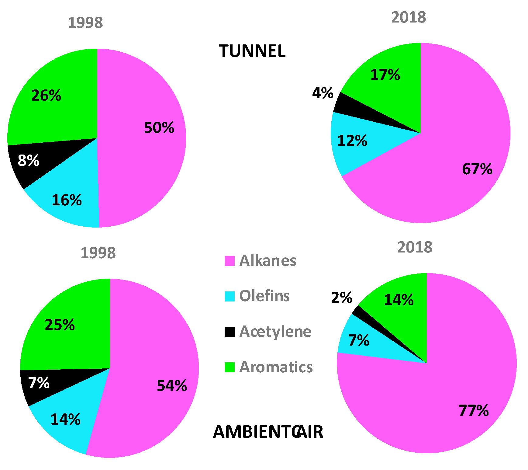
3.2. Exhaust Profiles of the Volatile Organic Compounds

A statistical study was carried out in order to determine the significant differences between the VOCs sampled in the two tunnels, and the differences between the two methods to collect the samples (instantaneous and 2 h-integrated). As the concentrations had significant variations, the composition of the species was obtained as wt%. The data were used for the Mann–Whitney test (α < 0.05) to determine possible significant differences. Data from instantaneous samples from the Mixcoac and Chapultepec tunnels were compared with the Chapultepec results of the 2 h-integrated samples. The comparison was made, first among the organic groups of which the results proved that there were no significant differences and then compound by compound (of the 54 analyzed) between the two groups (instantaneous and integrated samples). The results showed that there were no significant differences among the data in 95% of the compounds. Consequently, a unique tunnel emission profile was constructed. This profile represents a signature of the vehicular exhaust emissions.
The concentrations and compositions of the analyzed VOCs emitted by vehicles in the tunnel are shown in Table 2 and are compared with the VOC compositions in the ambient air, as well as with the concentrations and profiles obtained in 1998 by Mugica et al. [37,38]. Of the 54 compounds analyzed, only 46 proved to be consistent in the two periods. The VOC concentrations varied in every sampling due to the different number of vehicles. The tunnels concentrations were up to 9 times greater than those found in the ambient air, because the exhaust emission is concentrated in the confined area. The VOC concentrations in the Chapultepec tunnel were up to four times larger than in the Mixcoac tunnel, since the traffic in the first one was heavier. Most abundant VOCs in the tunnel were propane, nbutane, ipentane, toluene, and ethylene, while the most abundant compound in the ambient air was propane followed by toluene, ipentane, butane, and nhexane. In both cases, the abundances were different for 1998 and 2018, showing that the exhaust emission profiles have changed due to modifications in the vehicular technologies and gasoline composition. Despite that in 2018 the number of vehicles traversing during the experiment was 2.4 times higher than in 1998, the VOC concentration values decreased inside the tunnel from 3772 μgm−3 (1998) to 1167 μgm−3 (2018), while outside the tunnel decreased from 1165 μgm−3 to 263 μgm−3, which means that a better air quality was attained compared to 20 years ago. One of the most important reasons of high vehicular emissions in 1998 was that the age of many vehicles was more than 20 years, they had not catalytic converters and used the old carburetor technologies. The achievement in the reduction of emissions for air quality improvement is also due to different strategies such as the mandatory use of catalytic converters and the imposition of limits on fuel volatility to control the VOC emissions [19]. Another measure was the stringent automobile emission standards that in the case of hydrocarbons was reduced from 200–600 ppm (NOM-041-SEMARNAT-1999) to 100–300 ppm (NOM-041-SEMARNAT-2015). New parameters and methodologies to measure combustion efficiency and CO2 emissions in new light-duty vehicles (NOM-163-SEMARNAT-ENER-SCFI-2013) were introduced. In addition, the city implemented a mandatory twice-per-year vehicle verification, a circulation restriction to heavy load-vehicles and vehicular technological improvements. New public transport was also offered [20,23].
The isoprene was almost six times greater in the ambient air than in the tunnels, since this compound is produced by the vegetation. Inside the tunnels, the percentages of the ethylene, acetylene, propylene, benzene, ethylbenzene and xylenes, among others were 2.4, 2, 1.9, 1.7, 3.7, and 5.5 greater (respectively) than in the ambient air; these differences were also detected in 1998.
The high concentrations of propane, butene and ibutane which are components of LP gas, the fuel commonly used in residences and restaurants, were observed in both periods, although in 1998, the concentrations of those compounds were six times higher in the ambient air than in the tunnels. On the contrary, the concentrations of those compounds in 2018 were higher inside the tunnels, suggesting that the measures taken to reduce LP gas leaks during handling, transportation, and storage in homes and commerce tanks, succeeded. Nevertheless, more actions should be implemented to minimize the leaks since the high ratio of propane to nbutane and ibutane measured in the ambient air and in the tunnel, implies that LP gas leaks are still an important source of propane, as found by Zavala et al. [19].
The comparison of the light-duty gasoline VOC profiles with other studies is complicated, since results are reported in different units (ppb, ppbC, µg m‒3, wt%, v/v%, mg km‒1, among others). Additionally, every study reports different species, and some include unknowns or oxygenated compounds. Table 3 displays the comparison of the five most abundant VOCs in exhaust emissions determined in several tunnel studies. It is possible to observe that every profile is different, none of the species are repeated throughout the studies and the most recurrent is the ipentane, followed by ethylene and toluene, but ranked differently. These differences are due to the fuel compositions and combustion efficiency attributed to several factors, as well as interferences due to vehicular emissions from the use of other fuels, such as diesel or LP gas. The variation in only 13 species shows the relevance that each city determines its own vehicular emission profiles for designing strategies to improve air quality.

3.3. Carbonyl Compounds in Exhaust Emissions

Many carbonyls are highly reactive in the atmosphere, contributing to ozone formation, peroxyacyl nitrates, and other photochemical air pollutants [42]. The carbonyls are emitted by mobile, stationary, and area sources, such as graphic arts and painting facilities.
Table 4 displays the average concentration of the main carbonyl compounds from the 36 cartridges analyzed. The formaldehyde and acetaldehyde accounted in all cases for more than 80% of total measured carbonyls. The formaldehyde was the most abundant carbonyl in tunnel samples, followed by the acetaldehyde and 2-propenal, while in the ambient air the most abundant was acetaldehyde, on average. The formaldehyde has been typically the most abundant carbonyl found in vehicle emissions, although others, such as the acetaldehyde, could be present in similar or greater quantities [43,44,45]. The carbonyls inside the tunnel are primary exhaust emissions, then their composition represent the emission profile of these compounds from vehicles. The formaldehyde and acetone concentrations in the tunnel were 2.7 times greater than in the ambient air, but the acetaldehyde in the tunnel was only 1.2 times greater. The 2-propenal (acrolein), propanal (propionaldehyde), and 2-butenal (crotonaldehyde), presented concentrations a little higher inside than outside the tunnel, suggesting that near to the sampling site there could be one or more sources of those compounds.
The comparison with measured carbonyls in 1998 only includes formaldehyde, acetaldehyde, and acetone, having total average concentrations of 145 µg m−3 and 41.07 µg m−3 for the tunnel and ambient air, respectively, which are 2.9 and 1.5 times greater than the sum of these three compounds in the 2018 study. The decrease in the formaldehyde levels in Mexico City was reported by Gruter et al. [46], with ranges between 23.9 µg m−3 in February and 12.7 µg m−3 in October, since temperature and solar radiation affect the atmospheric formation of the carbonyls [44].

3.4. Gasoline and Head Space Profiles

The Kruskal–Wallis test showed that the 15 different gasoline brands of Magna had not significant differences among them, and the same result was obtained for the 15 Premium gasoline samples. The differences between the organic group content of the Magna and Premium gasolines are shown in Figure 4, where results are presented in v/v% since the Mexican Standard considers those units. The head space profiles are different from whole gasoline ones, due to the different vapor pressures of the diverse compounds and also presented differences between the Magna and Premium fuels. The isoalkanes content was increased in HS gasolines whereas there was a substantial reduction in the aromatics in the two gasoline types with 6% in the Magna HS and 5% in the Premium HS, showing the importance of including the heavy aromatic compounds with low vapor pressure to avoid evaporation.
The Mann–Whitney test (α < 0.05) showed significant differences among the Magna and Premium gasoline compositions presented in Table 5, since the p values were less than 0.05 in 48 compounds from the 60 considered, although the oxygenated species were excluded.
Although the Magna and Premium gasolines have the same content of olefins and oxygenated compounds, the Magna gasoline has a higher content of alkanes, isoalkanes, and naphthenes in comparison with the Premium gasoline. In opposite, the aromatic compounds content is greater in the Premium gasoline with 24% vs. 20% in the Magna. It was worrying to note that 4 of the 15 Premium samples characterized exceeded the aromatic limit content (24.85 ± 11.20 v/v%) recommended in the NOM-016-CRE-2016, in order to achieve the octane index of 92.
The 10 most abundant compounds in whole gasoline were the 2-methylpentane, ipentane, 2,2,4 trimethylpentane, toluene, npentane, 4-methyl-cis-2-pentene, nhexane, 1,3 dimethyl benzene, and 1,2,4 trimethylbenzene. Except for the last two, the same compounds were the most abundant for the gasoline vapors, although in a different order. The nbutane and 2,2, dimethylbutane were also in the first 10 more abundant compounds in the HS gasolines. In general, from the 60 most abundant compounds, 48 were in the 2 profiles (whole and HS), but in a different sequence. The differences between profiles are mainly related to the olefins, finding 10 of them in the most abundant 60 compounds of the HS gasolines because of their high vapor pressures, versus the five olefins found in the whole gasolines. Regarding the benzene content, it has decreased since 1998, and all analyzed gasolines met the standard (0.51% v/v and 0.49% v/v for the Magna and Premium, respectively), although this standard should be reduced within the next years because it is a well-known carcinogenic compound.
The NOM 016-CRE-2016 states that the oxygen content for the MCMA should be 1.087% maximum of the total mass (wt%), and no gasoline surpassed that value. The oxygenated species content was very variable in each gasoline. Therefore, they were not included in the statistical study to determine significant differences among the different gasolines. The most abundant oxygenated compound in all gasolines was the tert-amyl methyl ether, known as TAME, with an average content of 0.5 ± 0.5 wt% in the Magna and 0.4 ± 0.5 wt% in the Premium. The ethyl-tertbutyl-ether (ETBE) was the second oxygenated compound in abundance with 0.4 ± 0.1 wt% in the Magna whereas it was not present in the Premium, instead, the methyl tertbutyl-ether accounted for less than 0.05 wt%, and the third oxygenated compound was methanol with 0.1 ± 0.1 wt% in the Magna and 0.1 ± 0.1 wt% in the Premium. Other oxygenated compounds were found in minimal quantities in both types of gasolines, such as acetone, di-isopropyl ether, npropanol, and ethanol with minimum and maximum contents of 0–0.05 wt% and 0.01–0.04 wt% for the Magna and the Premium, respectively.
The composition of gasoline has important implications on air quality. First, because a fraction of the fuel is not burnt by the engine and goes directly to the catalytic converters, which even when they are highly efficient, still emit into the environment an uncatalyzed fraction. Second, the organic compounds having higher vapor pressures evaporate during filling of vehicle tanks, in spillages or leaks due to careless handling, and during overland transportation of fuels. In view of this, it is necessary to become acutely aware that some organic compounds are toxic. Third, a certain amount of ozone will be formed depending on the reactivity of components. The results obtained show that all gasolines sampled have the same composition; however, it is likely that in the next few years different gasoline compositions will begin to be distributed, so monitoring them will be essential. The formulation of new gasolines with lower content of toxic and reactive substances, such as olefins reduction should be part of the programs to improve air quality.

3.5. Ozone Formation Potential

Figure 5 depicts the relative contribution of different VOC groups to the OFP in the tunnels and in ambient air in the 1998 and 2018 campaigns, as well as the contributions of gasoline vapors in 2018. In the tunnels and HS gasolines, the olefins are the most significant VOCs for the production of ozone. The most evident difference in the contribution to the OFP during the two periods inside the tunnel was the decrease of the aromatic percent from 1998 (38%) to 2018 (29%) due to the changes in the gasoline compositions, then in 2018, OFP contributions of the alkanes, unsaturated (acetylene + olefins), and carbonyls increased. The great differences were observed for the ambient air, in 1998 the most reactive species were the aromatics followed by the olefins, while the carbonyls in 2018 displayed the highest contributions, showing again the effect of modifications to the composition of the gasolines. For the 1998 and 2018 campaigns, the total average OFP values inside the tunnels were 3.82 and 1.38 g O3 m−3 per gram of VOC, respectively, which means more than 60% an average of OFP, whereas in the ambient air the reduction was almost 67%, which also underlines the air quality improvement as a result of enforcing the strategies mentioned in the MCMA. Regarding the VOC groups contribution to the OFP in the HS gasoline that represents the gasoline evaporation, it is grievous to note that from 1998 to 2018, the aromatic and olefin contributions to ozone formation have increased from 3.8% to 9% and from 43.6% to 62%, respectively.
The ranking of main VOCs contributors from the HS to ozone production were as follows: 4-methyl-2-pentene, ipentane, xylenes, 2-methyl-pentane, 2-methyl-2-butene, and toluene [47]. Although the results obtained in the tunnels and in the ambient air showed that the OFP had a substantial diminishment, the ubiquitous aromatic compounds are considered important contributors to the secondary formation of organic aerosol (SOA) [48], then, more reductions are needed to achieve a better air quality. Thus, it could be possible to reduce these compounds and olefins by increasing some isoalkanes to maintain the octane index within the standard, which would be an exciting challenge to design less reactive and less toxic gasolines, as a new strategy.
The main contributing species to the photochemical formation of ozone emitted in the tunnels in 2018 were: ethylene, propylene, m/p xylene, 1-butene, toluene, 1,2,4 trimethylbenzene, propane, o-xylene, and ipentane, as can be seen in Figure 6 where their percentages are compared with the 22 most abundant VOCs, accounting for 80% of the exhaust emissions from the tunnels.

4. Discussion

4.1. Volatile Organic Compounds Profiles

The comparison of this research with the reported values of a similar study performed in the Chapultepec tunnel in 1998 [37], shows that the strategies applied in Mexico City related to mandatory incorporation of the catalytic converter, the fuel injection devices, and the annual engines verification and fuels improvement, have rendered the reduction of the olefins (from 16% to 12%), acetylene (from 8 to 4%), and aromatic compounds (from 26% to 17%) which are more toxic and reactive for the ozone formation.
The population increase from 16.7 million in 1998 to 21.4 million inhabitants in 2016 (last official report) [49], is reflected in a fleet increase from 2.7 million to 5.8 million vehicles [50]. The effectiveness of the last 20 years measures can also be gathered from the VOC concentrations reduction of around 70 and 75% inside and outside the tunnel, respectively. The main species from vehicle emissions measured in a Nanjing tunnel, in China, were ethane, ethylene, propane, ipentane, acetylene, and toluene that, except for ethane, the abundance of the VOCs are similar to those measured in this study; however, it is worrisome to note that the average of benzene and toluene concentrations in the MCMA tunnels were 4.4 and 6.4 times higher than those reported at the exit of that Chinese tunnel [35]. The same situation occurs when the results of this study are compared with the measured concentrations in 2015 at the exit of a tunnel in Hong Kong [51] and with the levels of quantified VOCs in other three Chinese tunnels in Beijing, Tianjin, and Nanjing [25]. The high concentrations of VOCs in the Chapultepec tunnel compared with those reported from other countries can be attributed to the low speeds of the vehicles in the tunnel, since at peak times the cars stop every 4 minutes by the traffic light located at short distance from the exit of the tunnel. A study performed in Hong Kong reported that the VOC emissions from light-duty gasoline vehicles were in average 2151 mg km−1 in the idle state, but when the speed was 25 km h‒1 and 50 km h−1, decreased to 29 and 7 mg km−1, respectively [52], the increase of emissions at low speeds had been reported in a tunnel study from California [53].
The case of toluene is interesting, since in 2018 the composition percent was 1.5% higher outside the tunnels than inside, unlike in 1998 where the abundance of toluene was 2.3% higher inside the tunnels than outside. This result is due to the reduction of toluene in gasolines and from other toluene sources, namely as solvent in paints and printing inks, which are more important sources of toluene in the air than in vehicular emissions [21]. Benzene average concentrations in the ambient air in 1998 were 17.66 µg m−3, and those high concentrations in the atmosphere were measured in the MCMA in 2000–2001 by Sosa et al. [54], with concentrations up to 19 µg m−3. Since 2001, the decrease of ambient air benzene and other aromatic compounds was reported by other researchers [20,23], which related this fact with the modification of fuels bearing now lower contents of aromatics and olefins, the installation of vapor recovery systems in fuel service stations, and improved car technology that brought about more efficient combustion, since most vehicles have fuel injection devices and other improvements, as reported recently [19]. Nevertheless, in comparison with other countries, the concentrations of aromatics in the MCMA are higher than those found in Austin, Texas in 2012 (up to 0.14 µg m−3 for benzene and up to 1.5 µg m−3 for toluene) [55].
The greater abundance of acetaldehyde than formaldehyde in the ambient air found in this study was reported by Kanjanasiranont et al. [45], who quantified an average of 43.13 µg m−3, and 17.44 µg m−3, respectively with larger standard deviations also in the ambient air during a exposure study of police personnel, while the propanal concentrations were 8.4 µg m−3; these 3 carbonyls had higher concentrations than those quantified in the tunnel observed here. Conversely, Aung et al. [56], measured formaldehyde concentrations from 3.7 to 7.4 µg m−3 and acetaldehyde concentrations from 2 to 4.7 µg m−3 in Myanmar, which are lower levels than those found in this study. Table 6 displays the correlations among the different carbonyl compounds in the tunnel with a significance level (α) of 0.05 by means of the r of Spearman. The positive strong correlations among them are observed (p < 0.05), thus pointing out at the same source; there is also a high correlation with the acetylene, a well-known vehicular exhaust marker, revealing the same origin. The exception was propanal (propionaldehyde) with a very weak positive correlation with the other carbonyls, that suggests other external sources, since its concentrations in the ambient air are quite similar to those in the tunnel. The formaldehyde/acetaldehyde ratios usually fluctuate from 1 to 2 in urban areas, though in rural ones the variation is around 10; the vehicular traffic is the primary source in winter while in summer, the carbonyls originate from the photochemical reactions in addition to exhaust emissions [57]. The mentioned ratio has been applied as an indicator of carbonyl-anthropogenic sources, although other authors indicate that ratios could vary broadly in urban sites [58]. In this study, the average formaldehyde/acetaldehyde in the tunnel was 1.6 ranging between 1 to 2.7, while in the ambient air the variations were large with an average of 1.1, ranging between 0.8 to 2.2; this last ratio in the ambient air is a little higher than the 0.99 reported for light duty vehicles in São Paulo, Brazil. In that country, fuels have different composition, like 75–80% gasoline and 20–25% ethanol [59]. A decrease of the formaldehyde/acetaldehyde ratio from 3.9 (1999) to 0.65 (2010) in a tunnel in California was attributed to the increased use of ethanol in fuels to 10% in 2010 [60,61].

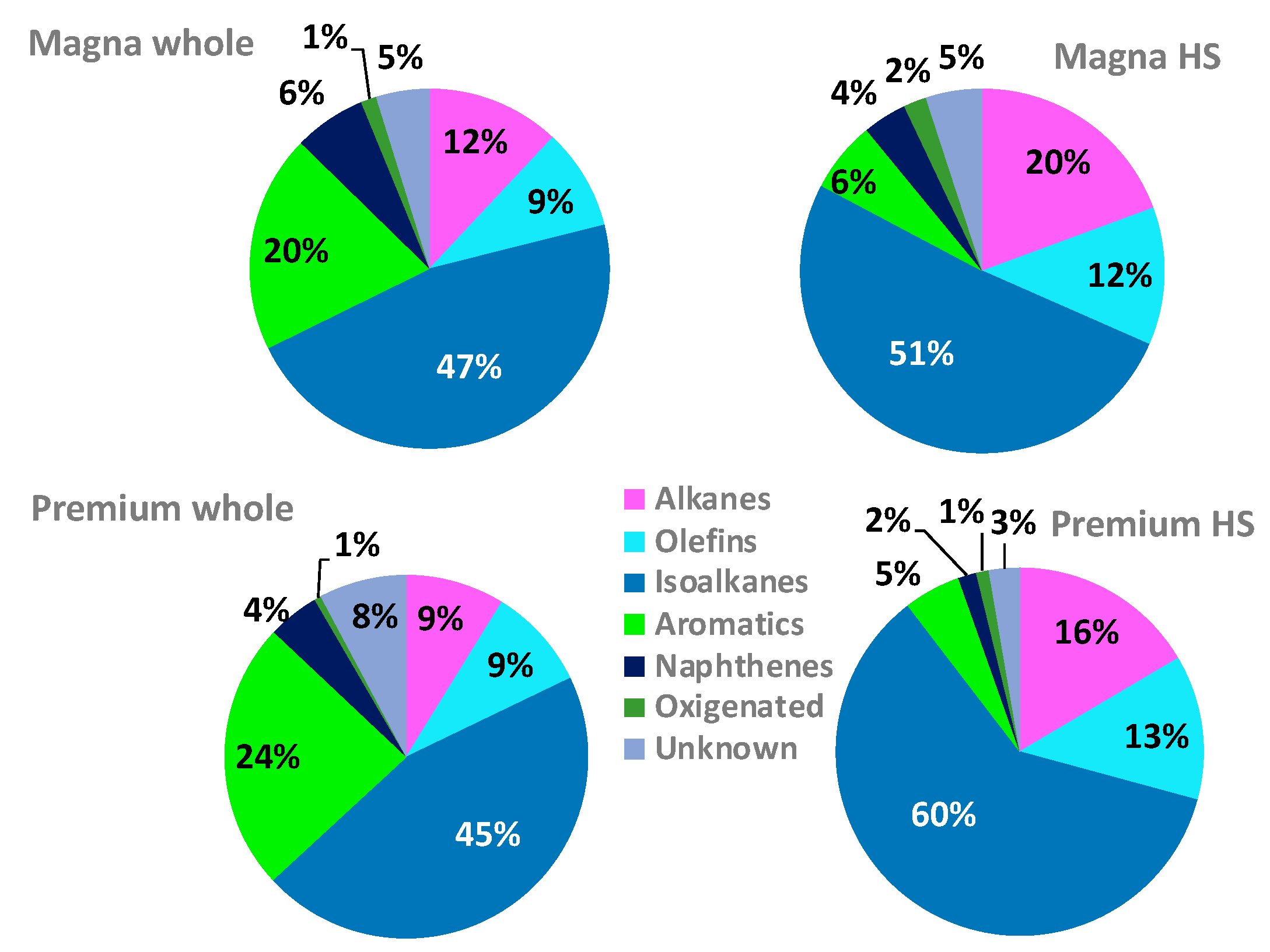
4.2. Gasoline and Head Space Profiles

In comparison with the Magna Sin gasoline in 1998, the most important change was in the aromatics and olefins content in order to attain lower VOC emissions. The aromatic content was 22.4% in the Magna Sin gasoline, albeit for 2018 it decreased to 20%; however, the olefins had an important increment from 3.4% to 9%. Nonetheless, the most toxic aromatic compounds: benzene, toluene, ethylbenzene, and xylenes, decreased their content from 1.1% to 0.6%, from 7.5% to 5%, from 1.3% to 1.2%, and from 7.1% to 4.8%, respectively, as a result of the changes in gasoline formulations. Several studies have shown that the reduction in the aromatic compounds in gasolines, lowers the VOC emissions, whereas a smaller effect is observed when the olefin content diminished; moreover, another gasoline reformulation action taken in the MCMA after 2010 was the reduction of sulfur content to 30 ppm to improve the performance of the catalytic converters [62].

4.3. Ozone Formation Potential

The most critical VOCs for the ozone production in 1998 and 2018 are shown in Figure 7. The ethylene was the highest contributor for the OFP in the tunnels exhaust emissions in both years followed by the toluene in 1998, but by the propylene in 2018, since the reduction of toluene in gasolines was one of the government strategies. The next compounds were m/p xylenes; 1-butene ranked 20 in 1998, but 4th in 2018 showing an important modification resulting from the new composition of gasolines. A study conducted in a tunnel in Southern China, reported that the VOCs making the most considerable contribution to OFP were the ethylene, propylene, m/p xylene, and toluene [35], which are also the most important contributors in this study.
Concerning the VOCs in the ambient air, the most important compounds for ozone production in 2018 were: toluene, 1-butene, isoprene, ethylene, propylene, propane, ipentane, and nbutane, similar to the ranking in 1998. It should stand out that although the propane and butane MIRs are smaller (0.46 and 1.08 gO3/gVOC), in comparison with other compounds, they are always in the twelve top places of a reactivity rank-like scale, because apart from the fact that they are produced during combustion, they are the principal components of LP gas, a commodity fuel, as mentioned before. In general, these results agree with those reported in other studies in the MCMA, such as that performed in 2005–2006, where the highest contributors to the OFP were: propylene, toluene, cis-2-butene, ethylene and m-xylene [18,20], whereas [19] Zavala et al. (2020) reported the reduction of VOC-OH reactivity in the city, estimated from 2014 to 2018, in comparison with 2006 levels and attributed the effect to the reduction the VOC emissions from mobile sources, where the most important species for ozone production were toluene, ethylene, propylene, npropane, isoprene, other alkenes and aromatics.

5. Conclusions

The volatile organic compound concentrations and profiles measured in the MCMA tunnels in 2018 showed significant differences with those reported 20 years ago, showing an important improvement in the MCMA air quality, since total the VOC concentrations were reduced from 3772 to 1157 µg m−3 despite the duplicated vehicular fleet. Although LP gas components still have a relevant contribution to the total VOCs, unlike 1998 measurements, the amount inside the tunnels was higher than outside, showing that strategies designed to reduce leaks were efficacious.
The aromatic and olefin contents in exhaust emissions decrease in the last 20 years from 26 to 17% and from 16 to 12%, respectively, whereas acetylene content, a gasoline combustion marker, decreased from 8 to 4%. The carbonyls in the tunnel diminished almost 3 times and around 1.5 times in the ambient air. The current light-duty vehicular emissions composition is less toxic than 20 years ago, although it still represents a health risk for the population.
Despite the existence of a fuel opened marked in Mexico, there were no differences among different gasoline brands, although the differences between Magna and Premium gasolines were evident.
The ozone formation potential was also reduced by 64% and 68% in the tunnels and ambient air, respectively, from 1998, implying a less reactive urban atmosphere and a better air quality. The results of this study reveal that the programs, policies, and strategies put forward in the last 20 years for the air quality improvement were effective in reducing exhaust emissions and gasoline vapors. However, more aggressive measures should be taken, especially in the fuels composition to avoid the multiple ozone exceedances in the city every year.
Although the exhaust VOC mixture emitted has currently less photochemical reactivity as well as that of the VOC ambient air mixture, the reduction in olefins in exhaust emissions could be a significant achievement, through the design of new gasolines, with less olefin content, such as in California where the maximum allowed in liquid gasolines is 4%, as compared with the 10% allowed in Mexico. This action should be enacted and enforced not only to decrease ozone formation potency but to reduce the health risk for the MCMA inhabitants.

Author Contributions

Conceptualization, V.M.-Á., and V.H.P.-F.; validation, S.B.-J. and V.G.-L.; formal analysis, J.F.-L.; investigation, V.M.-Á. and A.M.-R.; conducted VOCs analysis, M.M.-R.; conducted monitoring, gasoline, and HS analyses A.M.-R; conducted carbonyl analyses, R.G.-M.; conducted the project administration and funding acquisition V.M.-Á. All authors have read and agreed to the published version of the manuscript.

Funding

This research was funded by the Secretary of Education, Science, Technology and Innovation of Mexico City (SECTEI by its Spanish acronym), grant number 099/2017 and A.M.-R. thanks for her graduate scholarship from CONACYT.

Acknowledgments

Authors thank the contribution of Jorge Palma and Nathaly Tello for help in monitoring and analyses.

Conflicts of Interest

The authors declare no conflict of interest.

References

  1. Rumchev, K.; Spickett, J.; Bulsara, M.; Phillips, M.; Stick, S. Association of domestic exposure to volatile organic compounds with asthma in young children. Thorax 2004, 59, 746–751. [Google Scholar] [CrossRef] [PubMed] [Green Version]
  2. Jerrett, M.; Burnett, R.T.; Pope, C.A., 3rd; Ito, K.; Thurston, G.; Krewski, D.; Shi, Y.; Calle, E.; Thun, M. Long-term ozone exposure and mortality. N. Engl. J. Med. 2009, 360, 1085–1095. [Google Scholar] [CrossRef] [PubMed] [Green Version]
  3. Haick, H.; Broza, Y.Y.; Mochalski, P.; Ruzsanyi, V.; Amann, A. Assessment, origin, and implementation of breath volatile cancer markers. Chem. Soc. Rev. 2014, 43, 1423–1449. [Google Scholar] [CrossRef] [PubMed] [Green Version]
  4. Riojas-Rodriguez, H.; Álamo-Hernández, U.; Texcalac-Sangrador, J.L.; Romieu, I. Health impact assessment of decreases in PM10 and ozone concentrations in the Mexico City Metropolitan Area. A basis for a new air quality management program. Salud Publica Mex. 2014, 56, 579–591. [Google Scholar] [CrossRef]
  5. Feng, Z.; Hu, E.; Wang, X.; Jiang, L.; Liu, X. Ground-level O3 pollution and its impacts on food crops in China: A review. Environ. Pollut. 2015, 199, 42–80. [Google Scholar] [CrossRef] [PubMed]
  6. Cohen, A.J.; Brauer, M.; Burnett, R.; Anderson, R.; Frostad, J.; Estep, K.; Balakrishnan, K.; Brunekreef, B.; Dandona, L.; Dandona, R.; et al. Estimates and 25-year trends of the global burden of disease attributable to ambient air pollution: An analysis of data from the Global Burden of Diseases Study 2015. Lancet 2017, 389, 1907–1918. [Google Scholar] [CrossRef] [Green Version]
  7. Zhong, L.; Lee, C.S.; Haghighat, F. Indoor ozone and climate change. Sustain. Cities Soc. 2017, 28, 466–472. [Google Scholar] [CrossRef]
  8. Maas, R.; Grennfelt, P. (Eds.) Towards Cleaner Air Scientific Assessment Report 2016 EMEP Steering Body and Working Group on Effects of the Convention on Long-Range Transboundary Air Pollution; RIVM: Oslo, Norway, 2016. [Google Scholar]
  9. Fujita, M.E.; Campbell, E.D.; Zielinska, B.; Chow, C.J.; Lindhjem, E.C.; DenBleyker, A.; Bishop, A.G.; Schuchman, G.B.; Stedman, H.D.; Lawson, D. Comparison of the MOVES2010a, MOBILE6.2, and EMFAC2007 mobile source emission models with on-road traffic tunnel and remote sensing measurements. J. Air Waste Manag. 2012, 62, 1134–1149. [Google Scholar] [CrossRef] [Green Version]
  10. Duncan, B.N.; Yoshida, Y.; Olson, J.R.; Sillman, S.; Martin, R.V.; Lamsal, L.; Hu, Y.; Pickering, K.E.; Retscher, C.; Allen, D.J.; et al. Application of OMI observations to a space-based indicator of NOx and VOC controls on surface ozone formation. Atmos. Environ. 2010, 44, 2213–2223. [Google Scholar] [CrossRef] [Green Version]
  11. Carter, W.P.L. Development of the SAPRC-7 Chemical Mechanism and Updated Ozone Reactivity Sales: Final Report to the California Air Resources Board Contract No. 03-318; University of California: Riverside, CA, USA, 2009. [Google Scholar]
  12. Siciliano, B.; Dantas, G.; da Silva, C.M.; Arbilla, G. Increased ozone levels during the COVID-19 lockdown: Analysis for the city of Rio de Janeiro, Brazil. Sci. Total Environ. 2020, 737, 139765. [Google Scholar] [CrossRef]
  13. Sicard, P.; De Marco, A.; Agathokleous, E.; Feng, Z.; Xu, X.; Paoletti, E.; Rodriguez, J.J.D.; Calatayud, V. Amplified ozone pollution in cities during the COVID-19 lockdown. Sci. Total Environ. 2020, 735, 139542. [Google Scholar] [CrossRef] [PubMed]
  14. Ordóñez, J.M.; Garrido-Perez, R.; García-Herrera, R. Early spring near-surface ozone in Europe during the COVID-19 shutdown: Meteorological effects outweigh emission changes. Sci. Total Environ. 2020, 747, 141322. [Google Scholar] [CrossRef] [PubMed]
  15. Shi, X.; Brasseur, G.P. The response in air quality to the reduction of Chinese economic activities during the COVID-19 outbreak. Geophys. Res. Lett. 2020, 47, 1–8. [Google Scholar] [CrossRef] [PubMed]
  16. SEDEMA. Secretaría del Medio Ambiente. Bases de datos—Red Automática de Monitoreo Atmosférico (RAMA). Secretaría de Medio Ambiente, Mexico City. (Mexico City Database of the Automatic Atmospheric Monitoring Network). 2020. Available online: http://www.aire.cdmx.gob.mx/default.php (accessed on 22 September 2020).
  17. Kanda, I.; Basaldud, R.; Magaña, M.; Retama, A.; Kubo, R. Comparison of ozone production regimes between two Mexican cities: Guadalajara and Mexico City. Atmosphere 2016, 7, 91. [Google Scholar] [CrossRef] [Green Version]
  18. Jaimes-Palomera, M. Diseño del Monitoreo de Compuestos Precursores de Ozono en la Atmósfera de la Ciudad de México y su Área Metropolitana. Ph.D. Thesis, UNAM, Mexico City, Mexico, 18 January 2017. [Google Scholar]
  19. Zavala, M.; Brune, W.H.; Velasco, E.; Retama, A.; Cruz-Alavez, L.A.; Molina, L.T. Changes in ozone production and VOC reactivity in the atmosphere of the Mexico City Metropolitan area. Atmos. Environ. 2020, 238, 117747. [Google Scholar] [CrossRef]
  20. Garzón, J.P.; Huertas, J.I.; Magaña, M.; Huertas, M.E.; Cárdenas, B.; Watanabe, T.; Maeda, T.; Wakamatsu, S.; Blanco, S. Volatile organic compounds in the atmosphere of Mexico City. Atmos. Environ. 2015, 119, 415–429. [Google Scholar] [CrossRef] [Green Version]
  21. SEDEMA. Secretaría del Medio Ambiente. Calidad del Aire en la Ciudad de México. Informe 2017. (Air Quality Report in Mexico City). 2017. Available online: http://www.aire.cdmx.gob.mx/descargas/publicaciones/flippingbook/informe_anual_calidad_aire_2017/mobile/#p=8 (accessed on 12 August 2020).
  22. Velasco, E.; Retama, A. Ozone’s threat hits back Mexico City. Sustain. Cities Soc. 2017, 31, 260–263. [Google Scholar] [CrossRef]
  23. Jaimes-Palomera, M.; Retama, A.; Elias-Castro, G.; Neria-Hernández, A.; Rivera-Hernández, O.; Velasco, E. Non-methane hydrocarbons in the atmosphere of Mexico City: Results of the 2012 ozone-season campaign. Atmos. Environ. 2016, 132, 258–275. [Google Scholar] [CrossRef] [Green Version]
  24. Watson, J.G.; Chow, J.; Pace, T.G. Chemical mass balance. In Receptor Modeling for Air Quality Management, Data Handling; Science and Technology; Hopke, P.K., Ed.; Elsevier Science: New York, NY, USA, 1991. [Google Scholar]
  25. Song, C.; Liu, Y.; Sun, L.; Zhang, Q.; Mao, H. Emissions of volatile organic compounds (VOCs) from gasoline- and liquified natural gas (LNG)-fueled vehicles in tunnel studies. Atmos. Environ. 2020, 234, 117626. [Google Scholar] [CrossRef]
  26. Lonneman, W.A.; Seila, R.L.; Meeks, S.A. Non-methane organic composition in the Lincoln Tunnel. Environ. Sci. Technol. 1986, 20, 790. [Google Scholar] [CrossRef]
  27. McLaren, R.; Gertler, A.W.; Wittorff, D.N.; Belzer, W.; Dann, T.; Singleton, D.L. Real world measurements of exhaust and evaporative emissions in the Cassiar Tunnel predicted by chemical mass balance modeling. Environ. Sci. Technol. 1996, 30, 300–310. [Google Scholar] [CrossRef] [Green Version]
  28. Barrefors, G.; Petersson, G. Volatile hazardous hydrocarbons in a Scandinavian urban road tunnel. Chemosphere 1992, 25, 691–696. [Google Scholar] [CrossRef] [Green Version]
  29. Na, K.; Kim, Y.P.; Moon, I.; Moon, K.C. Chemical composition of major VOC emission sources in the Seoul atmosphere. Chemosphere 2004, 55, 585–594. [Google Scholar] [CrossRef] [PubMed]
  30. Lai, C.H.; Peng, Y.P. Volatile hydrocarbon emissions from vehicles and vertical ventilations in the Hsuehshan traffic tunnel, Taiwan. Environ. Monit. Assess. 2012, 184, 4015–4028. [Google Scholar] [CrossRef]
  31. Araizaga, A.; Mancilla, Y.; Mendoza, A. Volatile organic compound emissions from light-duty vehicles in Monterrey, Mexico: A tunnel study. Int. J. Environ. Res. 2013, 7, 277–292. [Google Scholar]
  32. Salameh, T.; Afif, C.; Sauvage, S.; Borbon, A.; Locoge, N. Speciation of non-methane hydrocarbons (NMHCs) from anthropogenic sources in Beirut, Lebanon. Environ. Sci. Pollut. Res. 2014, 21, 10867–10877. [Google Scholar] [CrossRef]
  33. Deng, C.; Zhang, M.; Liu, X.; Yu, Z. Emission characteristics of VOCs from on-road vehicles in an urban tunnel in eastern china and predictions for 2017–2026. Aerosol Air Qual. Res. 2018, 18, 3025–3034. [Google Scholar] [CrossRef]
  34. Huang, C.; Tao, S.S.; Lou, Q.; Hu, H.; Wang, Q.; Wang, L.; Li, H.; Wang, J.; Liu, Q.; Zhou, L. Evaluation of emission factors for light-duty gasoline vehicles based on chassis dynamometer and tunnel studies in Shanghai, China. Atmos. Environ. 2017, 169, 203. [Google Scholar] [CrossRef]
  35. Zhang, Y.; Yang, W.; Simpson, I.; Huang, X.; Yu, J.; Huang, Z.; Wang, Z.; Zhang, Z.; Liu, D.; Huang, Z.; et al. Decadal changes in emissions of volatile organic compounds (VOCs) from on-road vehicles with intensified automobile pollution control: Case study in a busy urban tunnel in south China. Environ. Pollut. 2018, 233, 806–819. [Google Scholar] [CrossRef]
  36. Marinello, S.; Lolli, F.; Gamberini, R. Roadway tunnels: A critical review of air pollutant concentrations and vehicular emissions. Transp. Res. D 2020, 86, 102478. [Google Scholar] [CrossRef]
  37. Mugica, V.; Vega, E.; Arriaga, J.L.; Ruiz, M.E. Determination of motor vehicle profiles for non-methane organic compounds in the Mexico City Metropolitan Area. J. Air Waste Manag. 1998, 48, 1060–1068. [Google Scholar] [CrossRef] [PubMed] [Green Version]
  38. Mugica, V.; Vega, E.; Ruiz, H.; Sánchez, G.; Reyes, E.C.A. Photochemical reactivity and sources of individual VOCS in Mexico City. Air Pollut. 2002, X, 209–217. [Google Scholar]
  39. USEPA. Compendium Method TO-11A. Determination of Formaldehyde in Ambient Air Using Adsorbent Cartridge Followed by High Performance Liquid Chromatography (HPLC); U.S. Environmental Protection Agency: Cincinnati, OH, USA, 1999.
  40. USEPA. Compendium Method TO-14A. Determination of Volatile Organic Compounds (VOCs) in Ambient Air Using Specially Prepared Canisters with Subsequent Analysis by Gas Chromatography; U.S. Environmental Protection Agency: Cincinnati, OH, USA, 1999.
  41. USEPA. Compendium Method TO-15. Determination of Volatile Organic Compounds (VOCs) in Air Collected in Specially-Prepared Canisters and Analyzed by Gas Chromatography/Mass Spectrometry (GC/MS); U.S. Environmental Protection Agency: Cincinnati, OH, USA, 1999.
  42. Atkinson, R. Atmospheric chemistry of VOCs and NOx. Atmos. Environ. 2000, 34, 2063–2101. [Google Scholar] [CrossRef]
  43. Wagner, T.; Wyszyński, M.L. Aldehydes and ketones in engine exhaust emissions—A review. Proc. Inst. Mech. Eng. Part D J. Automob. Eng. 1996, 210, 109–122. [Google Scholar] [CrossRef]
  44. Ho, K.F.; Lee, S.C.; Tsai, W.Y. Carbonyl compounds in the roadside environment of Hong Kong. J. Hazard. Mater. 2006, 133, 24–29. [Google Scholar] [CrossRef] [PubMed]
  45. Kanjanasiranont, N.; Prueksasit, T.; Morknoy, D. Inhalation exposure and health risk levels to BTEX and carbonyl compounds of traffic policeman working in the inner city of Bangkok, Thailand. Atmos. Environ. 2017, 152, 111–120. [Google Scholar] [CrossRef]
  46. Grutter, M.; Flores, E.; Andraca-Ayala, G.; Báez, A. Formaldehyde levels in downtown Mexico City during 2003. Atmos. Environ. 2005, 39, 1027–1034. [Google Scholar] [CrossRef]
  47. Mugica-Álvarez, V.; Martínez-Reyes, C.A.; Santiago-Tello, N.M.; Martínez-Rodríguez, I.; Gutiérrez-Arzaluz, M.; Figueroa-Lara, J.J. Evaporative volatile organic compounds from gasoline in Mexico City: Characterization and atmospheric reactivity. Energy Rep. 2020, 6, 825–830. [Google Scholar] [CrossRef]
  48. Wu, W.; Zhao, B.; Wang, S.; Hao, J. Ozone and secondary organic aerosol formation potential from anthropogenic volatile organic compounds emissions in China. J. Environ. Sci. 2017, 53, 224–237. [Google Scholar] [CrossRef]
  49. SEDEMA. Secretaría del Medio Ambiente. Inventario de Emisiones de la CDMX 2016. Secretaría de Medio Ambiente. 2016. Available online: http://www.aire.cdmx.gob.mx/descargas/publicaciones/flippingbook/inventario-emisiones-2016/mobile/ (accessed on 15 March 2020).
  50. INEGI. Parque Vehicular. Instituto Nacional de Estadística, Geografía e Informática. 2019. Available online: https://www.inegi.org.mx/temas/vehiculos (accessed on 10 October 2019).
  51. Cui, L.; Wang, X.L.; Ho, K.F.; Gao, Y.; Liu, C.; Hang, H.S.S.; Li, H.W.; Lee, S.C.; Wang, X.M.; Jiang, B.Q.; et al. Decrease of VOC emissions from vehicular emissions in Hong Kong from 2003 to 2015: Results from a tunnel study. Atmos. Environ. 2018, 177, 64–74. [Google Scholar] [CrossRef]
  52. Guo, H.; Zou, S.C.; Tsai, W.Y.; Chan, L.Y.; Blake, D.R. Emission characteristics of nonmethane hydrocarbons from private cars and taxis at different driving speeds in Hong Kong. Atmos. Environ. 2011, 45, 2711–2721. [Google Scholar] [CrossRef] [Green Version]
  53. Kean, A.J.; Harley, R.A.; Kendall, G.R. Effects of vehicle speed and engine. Load on motor vehicle emissions. Environ. Sci. Technol. 2003, 37, 3739–3746. [Google Scholar] [CrossRef] [PubMed] [Green Version]
  54. Sosa, E.R.; Bravo, A.H.; Mugica, A.V.; Sanchez, A.P.; Bueno, L.E.; Krupa, S. Levels and source apportionment of volatile organic compounds in Southwestern area of Mexico City. Environ. Pollut. 2009, 157, 1038–1044. [Google Scholar] [CrossRef] [PubMed]
  55. Durrenberger, C.J.; Spinhirne, J.P.; McGaughey, G.; McDonald-Buller, E.C. VOC Monitoring in the Austin Area: 2012; Center for Energy and Environmental Resources of the University of Texas: Austin, TX, USA, 2013. [Google Scholar]
  56. Aung, W.Y.; Noguchi, M.; Yi, E.E.P.N.; Thant, Z.; Uchiyama, S.; Shwe, T.T.W.; Kunugita, N.; Mar, O. Preliminary assessment of outdoor and indoor air quality in Yangon city, Myanmar. Atmos. Pollut. Res. 2019, 10, 722–730. [Google Scholar] [CrossRef]
  57. Possanzini, M.; Di Palo, V.; Petricca, M.; Fratarcangeli, R.; Brocco, D. Measurement of formaldehyde and acetaldehyde in the urban ambient air. Atmos. Environ. 1996, 30, 3757–3764. [Google Scholar] [CrossRef]
  58. Grosjean, D.; Grosjean, E. Airborne carbonyls from motor vehicle emissions in two highway tunnels. Res. Rep. Health Eff. Inst. 2002, 107, 5778. [Google Scholar]
  59. Nogueira, T.; de Souza, K.F.; Fornaro, A.; de Fatima Andrade, M.; de Carvalho, L.R.F. On-road emissions of carbonyls from vehicles powered by biofuel blends in traffic tunnels in the Metropolitan Area of Sao Paulo, Brazil. Atmos. Environ. 2015, 108, 88–97. [Google Scholar] [CrossRef]
  60. Kean, A.J.; Grosjean, E.; Grosjean, D.; Harley, R.A. On-road measurement of carbonyls in California light-duty vehicle emissions. Environ. Sci. Technol. 2001, 35, 4198–4204. [Google Scholar] [CrossRef] [Green Version]
  61. Gentner, D.R.; Worton, D.R.; Isaacman, G.; Davis, L.C.; Dallmann, T.R.; Wood, E.C.; Herndon, S.C.; Goldstein, A.H.; Harley, R.A. Chemical composition of gas phase organic carbon emissions from motor vehicles and implications for ozone production. Environ. Sci. Technol. 2013, 47, 11837–11848. [Google Scholar] [CrossRef]
  62. Schifter, I.; Díaz, L.; González, U.; González-Macías, C. Fuel formulation for recent model light duty vehicles in Mexico base on a model for predicting gasoline emissions. Fuel 2013, 107, 371–381. [Google Scholar] [CrossRef]
Figure 1. Location of the sampled tunnels.
Atmosphere 11 01339 g001
Figure 2. Concentration of the organic groups in the tunnels and ambient air.
Atmosphere 11 01339 g002
Figure 3. Comparison of the organic group compositions (wt%) in the Chapultepec tunnel and ambient air in 1998 [37] and 2018.
Atmosphere 11 01339 g003
Figure 4. General composition of whole and head space Magna and Premium gasoline v/v%.
Atmosphere 11 01339 g004
Figure 5. Contribution to ozone formation potential in tunnels and ambient air.
Atmosphere 11 01339 g005
Figure 6. Contributions of the most abundant compounds to ozone formation potential (OFP) measured in tunnels.
Atmosphere 11 01339 g006
Figure 7. Main VOC contributors to photochemical ozone formation in tunnels and ambient air.
Atmosphere 11 01339 g007
Table 1. Characteristics of the vehicular fleet.
Light Duty CarsVans and
Pick Ups
MotorcyclesBuses and
Diesel Trucks
Total Vehicles
Chapultepec
2018
Number%Number%Number%Number%
January 17372869.6100418.756010.45681.35360
January 18372867.6120021.85009.1881.65516
January 19301065.7887819.1959811.61902.14576
Average Chap3488.6 1027.4 553 82 5151
Mixcoac 2018
March 26222766.059817.754416.130.13372
March 27217768.474622.92738.640.133200
Average Mix220267.267220.3408.512.43.50.13286
2018.
Total Average
297467.5885.22049511.25114405
1998. Total Average
(3 days)
158887.71739.6442.460.31811
Table 2. Average and standard deviations of the concentrations and profiles.
CompoundTunnel 2018
Concentration Percent
Ambient Air 2018
Concentration Percent
Tunnel 1998 a
Concentration Percent
Ambient Air 1998 a
Concentration Percent
µg/m3%µg/m3%µg/m3%µg/m3%
ethane21.8 ± 9.41.9 ± 0.36.9 ± 0.92.6 ± 1.048.0 ± 12.11.3 ± 0.116.5 ± 7.21.4 ± 0.4
ethylene59.1 ± 23.35.1 ± 1.26.1 ± 3.32.1 ± 0.3201.4 ± 98.75.3 ± 0.432.4 ± 17.12.8 ± 0.3
propane258.6 ± 126.523.1 ± 6.591.0 ± 57.135.5 ± 10.5215.8 ± 106.75.7 ± 0.7258.0 ± 14722.2 ± 7.7
propylene30.2 ± 12.12.6 ± 0.73.9 ± 1.81.4 ± 0.3103.5 ± 23.62.7 ± 0.214.9 ± 3.61.3 ± 0.5
ibutane29.4 ± 11.22.5 ± 0.610.8 ± 4.74.1 ± 0.558.9 ± 13.21.6 ± 0.358.0 ± 13.74.9 ± 0.4
nbutane75.3 ± 27.66.5 ± 1.721.5 ± 7.48.3 ± 0.7180.0 ± 41.34.8 ± 0.7133.1 ± 61.911.4 ± 1.1
acetylene44.6 ± 19.23.8 ± 0.85.2 ± 1.91.9 ± 0.4380.8 ± 171.410.1 ± 1.248.7 ± 10.84.2 ± 0.3
1-butene27.6 ± 18.12.4 ± 0.87.2 ± 5.14.4 ± 3.610.6 ± 3.150.3 ± 0.010.6 ± 2.80.9 ± 0.3
trans-2-butene4.2 ± 2.50.4 ± 0.10.8±0.30.3±0.213.5 ± 2.90.4 ± 0.03.3 ± 6.00.3 ± 0.0
cis-2-butene3.4 ± 2.10.3 ± 0.10.8 ± 0.10.3 ± 0.211.5 ± 1.70.3 ± 0.03.9 ± 0.90.3 ± 0.0
ipentane73.2 ± 44.26.3 ± 1.318.9 ± 6.87.0 ± 4.9379.9 ± 19210.1 ± 1.2125.8 ± 71.410.8 ± 1.0
1-pentene4.3 ± 1.90.4 ± 0.11.2 ± 1.10.4 ± 0.311.4 ± 1.80.3 ± 0.02.9 ± 0.70.3 ± 0.0
nPentane36.0 ± 20.63.1 ± 0.68.9 ± 2.33.2 ± 2.0152.2 ± 65.74.0 ± 0.443.3 ± 9.93.7 ± 0.0
trans-2-pentene5.6 ± 3.10.5 ± 0.10.0 ± 0.00.0 ± 0.021.1 ± 4.60.6 ± 0.14.5 ± 0.90.4 ± 0.2
isoprene3.6 ± 1.00.3 ± 0.25.6 ± 3.91.8 ± 1.81.6 ± 0.50.1 ± 0.91.6 ± 0.40.1 ± 0.0
cis-2-pentene2.7 ± 1.40.2 ± 0.10.0 ± 0.00.0 ± 0.011.4 ± 3.90.3 ± 2.82.4 ± 0.50.2 ± 0.0
2,2-dimethylbutane3.3 ± 1.20.3 ± 0.10.3 ± 0.10.1 ± 0.03.2 ± 0.70.1 ± 0.05.6 ± 1.20.5 ± 0.0
cyclopentane12.2 ± 7.31.1 ± 0.22.2 ± 0.50.8 ± 0.411.6 ± 2.60.3 ± 0.32.4 ± 0.50.2 ± 0.0
2/3-methylpentane41.0 ± 26.03.5 ± 0.78.4 ± 3.12.9 ± 2.0155.7 ± 72.34.1 ± 0.230.0 ± 7.22.6 ± 0.0
nhexane33.1 ± 22.32.8 ± 0.610.0 ± 5.03.7 ± 2.7120.7 ± 48.73.2 ± 0.131.2 ± 7.12.7 ± 0.7
2,4-dimethylpentane10.5 ± 7.80.9 ± 0.30.5 ± 0.50.1 ± 0.138.8 ± 9.51.0 ± 0.03.4 ± 0.80.3 ± 0.0
methylcyclopentane16.0 ± 10.91.4 ± 0.32.3 ± 1.40.8 ± 0.65.5 ± 1.30.2 ± 0.06.8 ± 1.30.6 ± 0.1
benzene19.4 ± 10.51.7 ± 0.23.0 ± 0.71.0 ± 0.3119.7 ± 51.63.2 ± 0.217.7 ± 4.81.5 ± 0.1
2-methylhexane13.5 ± 9.11.2 ± 0.20.8 ± 0.30.3 ± 0.151.2 ± 12.61.4 ± 0.09.0 ± 2.10.8 ± 0.1
cyclohexane5.6 ± 3.30.5 ± 0.10.3 ± 0.30.1 ± 0.243.9 ± 16.51.2 ± 0.02.0 ± 0.50.2 ± 0.0
2,3-dimethylpentane11.9 ± 9.11.0 ± 0.30.4 ± 0.40.1 ± 0.145.2 ± 9.81.2 ± 0.04.3 ± 0.80.4 ± 0.0
3-methylhexane14.5 ± 9.91.2 ± 0.30.8 ± 0.40.2 ± 0.256.7 ± 7.51.5 ± 0.011.4 ± 2.71.0 ± 0.1
2,2,4-trimethylpentane58.1 ± 47.85.0 ± 1.75.1 ± 1.01.9 ± 0.8233.7 ± 114.36.2 ± 0.422.6 ± 5.31.9 ± 0.2
nheptane12.5 ± 8.21.1 ± 0.21.3 ± 1.20.5 ± 0.349.2 ± 12.01.3 ± 0.010.3 ± 3.00.9 ± 0.1
methylcyclohexane7.4 ± 5.30.6 ± 0.20.4 ± 0.40.1 ± 0.119.1 ± 2.40.5 ± 0.04.1 ± 1.30.3 ± 0.0
2,3,4-trimethylpentane19.0 ± 15.41.6 ± 0.50.8 ± 0.40.2 ± 0.293.9 ± 3.72.5 ± 0.111.0 ± 3.60.9 ± 0.1
2-methylheptane5.8 ± 4.60.5 ± 0.20.5 ±0.40.1 ± 0.121.9 ± 4.20.6 ± 0.14.1 ± 1.00.4 ± 0.0
toluene65.5 ± 41.105.6 ± 1.120.8 ± 15.17.1 ± 6.3347.7 ± 164.19.2 ± 0.279.9 ± 22.96.9 ± 0.2
3-methylheptane9.1 ± 6.70.8 ± 0.20.5 ± 0.40.1 ± 0.125.0 ± 6.40.7 ± 0.04.1 ± 0.80.4 ± 0.0
noctane6.5 ± 3.90.6 ± 0.20.8 ± 0.40.3 ± 0.228.1 ± 6.60.7 ± 0.46.2 ± 1.80.5 ± 0.0
ethylbenzene12.9 ± 7.41.1 ± 0.21.2 ± 1.00.3 ± 0.269.7 ± 15.01.9 ± 0.115.5 ± 4.61.3 ± 0.1
m/p-xylene40.5 ± 18.93.5 ± 0.62.8 ± 1.30.5 ± 0.5233.5 ± 123.76.2 ± 0.356.0 ± 18.14.8 ± 0.2
nnonane2.9 ± 1.20.3 ± 0.30.6 ± 0.60.2 ± 0.12.3 ± 0.60.1 ± 0.04.4 ± 1.50.4 ± 0.0
styrene2.9 ± 1.40.3 ± 0.31.0 ± 0.60.2 ± 0.213.3 ± 3.60.4 ± 0.03.6 ± 0.90.3 ± 0.0
o-xylene14.9 ± 9.51.3 ± 0.31.2 ± 1.10.3 ± 0.290.2 ± 23.72.4 ± 0.421.1 ± 6.81.8 ± 0.1
iprophylbenzene0.9 ± 0.70.1 ± 0.10.5 ± 0.50.1 ± 0.18.4 ± 2.00.2 ± 0.04.6 ± 2.30.4 ± 0.0
nprophylbenzene2.0 ± 1.80.2 ± 0.30.8 ± 0.40.2 ± 0.218.8 ± 4.30.5 ± 0.03.1 ± 2.00.3 ± 0.0
1,3,5 trimethylbenzene5.4 ± 3.30.46 ± 0.320.8 ± 0.70.2 ± 0.135.2 ± 7.70.9 ± 1.010.2 ± 3.60.9 ± 1.0
ndecane3.1 ± 2.90.26 ± 0.540.9 ± 0.50.3 ± 0.310.0 ± 2.60.3 ± 0.12.8 ± 1.50.2 ± 0.0
1,2,4-trimethylbenzene22.9 ± 16.62.0 ± 0.61.8 ± 1.10.5 ± 0.310.5 ± 3.60.3 ± 0.016.3 ± 4.91.4 ± 1.0
nundecane1.9 ± 1.50.2 ± 0.53.1 ± 2.31.5 ± 1.97.6 ± 1.60.2 ± 0.11.3 ± 0.60.1 ± 0.0
Total1156.6 262.7 3771.5 1165.3
a Mugica et al. [37,38].
Table 3. Comparison of most abundant volatile organic compounds (VOCs) in exhaust emissions in tunnel studies.
CityCountryAbundance
Ranking 1
Abundance
Ranking 2
Abundance
Ranking 3
Abundance
Ranking 4
Abundance
Ranking 5
Reference and Publication Year
SeoulKoreanbutaneethylenetolueneibutanem/p xylene[29] 2004
TaipeiTaiwanethyleneipentanepropyleneacetylene1-butene[30] 2012
MonterreyMexicoethyleneacethyleneipentanetoluenenbutane[31] 2013
BeirutLebanonipentanenbutanetoluenem/p xyleneibutane[32] 2014
NanjingChinaethaneethylenepropaneipentaneacetylene[35] 2018
BeijingChinaethyleneipentanetolueneacethylenenbutane[25] 2020
Mexico CityMexicoacethyleneipentanetoluene2,2,4 trimethylpentanem/p xylene[37] 1998
Mexico CityMexicopropanenbutaneipentanetolueneethyleneThis study
Table 4. Carbonyl compounds concentrations inside and outside the tunnel.
CompoundTunnel Concentrations
µg m−3
Composition
Tunnel
Ambient air Concentrations
µg m−3
Composition
Tunnel
Mean ± SDMin–Maxwt%Mean ± SDMin–Maxwt%
Formaldehyde30.3 ± 15.810.8–58.651.5 ± 6.111.3 ± 5.84.7–21.439.4 ± 10.5
Acetaldehyde19.2 ± 8.58.5–40.335.1 ± 2.616.2 ± 14.43.2–47.341.9 ± 1.3
2-Propenal3.8 ± 12.01.5–8.56.4 ± 0.83.4 ± 2.91–8.78.2 ± 4.7
Acetone1.1 ± 0.70.4–3.11.8 ± 0.050.4 ± 0.40.1–1.31.2 ± 0.7
Propanal1.8 ± 0.40.4–2.64.1 ± 0.211.6 ± 1.40.1–4.67.9 ± 6.2
2-Butenal0.7 ± 0.50.2–2.11.1 ± 0.150.5 ± 1.00.0–4.41.3 ± 1.5
∑carbonyls58.9 ± 3325.8–148.3 33.4 ± 22.69.9–81.8
Table 5. Composition of the whole and head space (HS) gasolines expended in Mexico City.
Compoundswt%
Magna
wt%
Premium
wt%
Magna HS
wt%
Premium HS
nbutane0.9 ± 0.40.8 ± 0.35.21 ± 2.95.5 ± 2.7
trans-2-butene0.1 ± 0.00.1 ± 0.10.3 ± 0.20.1 ± 0.1
ipentane7.1 ± 1.89.3 ± 3.621.1 ± 8.734.5 ± 9.1
2-methyl-1-butene0.3 ± 0.10.4 ± 0.20.0 ± 0.01.1 ± 0.3
1-pentene0.1 ± 0.00.2 ± 0.10.9 ± 0.50.5 ± 0.2
npentane4.1 ± 1.23.0 ± 1.09.3 ± 3.87.9 ± 2.8
trans-2-pentene0.4 ± 0.20.6 ± 0.20.8 ± 0.41.7 ± 0.3
cis-2-pentene0.2 ± 0.10.3 ± 0.10.5 ± 0.20.7 ± 0.2
trans-2-butene0.1 ± 0.00.1 ± 0.10.3 ± 0.20.4 ± 0.3
2-methyl-2-butene0.7±0.20.9±0.41.1±0.62.1±0.5
2,2-dimethylbutane0.7±0.50.7±0.31.6±1.40.9±0.4
cyclopentene0.1±0.00.1±0.00.3±0.20.2±0.1
2-methylpentane9.4 ± 1.99.4 ± 2.612.7 ± 4.414.0 ± 3.4
4-methyl-cis 2-pentene3.5 ± 0.73.1 ± 1.03.9 ± 1.53.7 ± 1.0
3-methylpentane2.2 ± 0.41.8 ± 0.62.2 ± 0.81.8 ± 0.6
nhexane2.8 ± 0.71.7 ± 0.82.3 ± 0.81.5 ± 0.6
3-methyl-cIs-2-pentene0.2 ± 0.10.2 ± 0.00.2 ± 0.20.2 ± 0.1
3,3-dimethylpentene-10.2 ± 0.10.3 ± 0.10.2 ± 0.10.2 ± 0.1
methylcyclopentane1.5 ± 0.31.0 ± 0.41.2 ± 0.40.8 ± 0.3
2,4-dimethylpentane1.1 ± 0.30.9 ± 0.30.7 ± 0.30.6 ± 0.2
1-methylcyclopentene0.2 ± 0.10.2 ± 0.10.2 ± 0.10.2 ± 0.0
benzene0.6 ± 0.10.6 ± 0.30.5 ± 0.20.4 ± 0.1
2-methylhexane1.6 ± 0.31.1 ± 0.50.8 ± 0.40.5 ± 0.2
cyclohexane0.8 ± 0.30.4 ± 0.20.6 ± 0.30.2 ± 0.1
t-amylmethyether0.5 ± 0.50.4 ± 0.40.4 ± 0.40.2 ± 0.1
2,3-dimethylpentane1.3 ± 0.40.9 ± 0.30.8 ± 0.40.4 ± 0.2
1t,3,dimethylcyclopentane0.5 ± 0.10.3 ± 0.10.3 ± 0.20.1 ± 0.0
3-methylhexane1.8 ± 0.31.2 ± 0.50.9 ± 0.40.5 ± 0.2
1c,3,dimethylcyclopentane0.3 ± 0.10.3 ± 0.10.3 ± 0.90.1 ± 0.0
2,2,4-trimethylpentane7.4 ± 3.96.8 ± 2.73.8 ± 2.32.5 ± 1.3
nheptane1.8 ± 0.31.0 ± 0.40.8 ± 0.40.3 ± 0.2
1,2-dimethylbenzene1.7 ± 0.42.2 ± 0.60.5 ± 0.70.3 ± 0.3
methylcyclohexane1.1 ± 0.40.6 ± 0.20.4 ± 0.30.2 ± 0.1
2,5-dimethylhexane1.0 ± 0.21.0 ± 0.30.4 ± 0.20.3 ± 0.2
2,4-dimethylhexane1.1 ± 0.31.2 ± 0.40.5 ± 0.30.3 ± 0.3
2,3,3-trimethylpentane2.2 ± 0.63.2 ± 1.60.9 ± 1.20.8 ± 0.7
2,3,4- trimethylpentane2.2 ± 0.62.7 ± 1.10.8 ± 0.60.7 ± 0.6
2-methyheptane0.8 ± 0.20.6 ± 0.20.3 ± 0.20.1 ± 0.1
2,2,5-trimethylhexane0.9 ± 0.30.8 ± 0.30.3 ± 0.30.2 ± 0.2
toluene5.0 ± 1.05.9 ± 1.71.9 ± 1.31.8 ± 1.3
2,3-dimethyhexane0.7 ± 0.20.7 ± 0.20.2 ± 0.20.2 ± 0.1
3-methyheptane0.7 ± 0.20.6 ± 0.20.3 ± 0.20.1 ± 0.1
noctane0.9 ± 0.20.6 ± 0.20.3 ± 0.30.1 ± 0.1
ethylbenzene1.2 ± 0.31.7 ± 0.50.4 ± 0.40.3 ± 0.3
1,3-dimethylbenzene3.0 ± 0.73.9 ± 1.21.0 ± 1.00.8 ± 0.8
1,4-dimethylbencene1.2 ± 0.31.4 ± 0.50.4 ± 0.40.4 ± 0.4
nnonane0.4 ± 0.20.3 ± 0.10.2 ± 0.10.1 ± 0.0
1,2-dimethylbencene0.6 ± 0.22.2 ± 0.60.5 ± 0.30.5 ± 0.5
ipropylbenzene0.1 ± 0.00.2 ± 0.10.0 ± 0.00.0 ± 0.0
npropylbenzene0.5 ± 0.10.5 ± 0.20.0 ± 0.00.1 ± 0.0
m-xylene1.6 ± 0.41.7 ± 0.80.5 ± 0.70.3 ± 0.3
p-xylene0.7 ± 0.20.8 ± 0.30.3 ± 0.30.2 ± 0.2
o-xylene0.6 ± 0.20.6 ± 0.30.2 ± 0.20.1 ± 0.1
1,3,5-tri-MeBenzene0.7 ± 0.20.8 ± 0.40.3 ± 0.30.2 ± 0.2
2-methylnonane0.4 ± 0.20.3 ± 0.20.2 ± 0.20.1 ± 0.1
ndecane0.2 ± 0.10.1 ± 0.10.1 ± 0.10.0 ± 0.0
1,2,4-trimethylbenzene2.5 ± 0.62.8 ± 1.40.7 ± 40.5 ± 0.6
1,2,3-trimethylbenzene0.6 ± 0.20.6 ± 0.30.2 ± 0.20.1 ± 0.1
1,3-diethylbenzene0.2 ± 0.00.2 ± 0.10.1 ± 0.00.0 ± 0.0
1,4-diethylbenzene0.3 ± 0.10.3 ± 0.20.1 ± 0.10.1 ± 0.0
Table 6. Spearman correlation (α < 0.05) among different carbonyls and acetylene in the tunnel.
FAAA2PAPA2B
Formaldehyde (FA)1.00
Acetaldehyde (AA)0.861.00
2-propenal (2P)0.920.831.00
Acetone (A)0.880.740.851.00
Propanal (PA)0.110.340.130.291.00
2-butenal (2B)0.920.830.890.820.281.00
Acetylene0.910.870.760.780.110.79
Statistically significant correlations with r > 0.7 are highlighted.
Publisher’s Note: MDPI stays neutral with regard to jurisdictional claims in published maps and institutional affiliations.

