Numerical Study on the Influence of Weir Construction on Near-Surface Atmospheric Conditions

Abstract

Changes in land use/land cover (LULC) have an impact on weather and climate. Gumi Weir in the Nakdong River Basin of South Korea was built and led to changes of LULC in the river in which the width of the river was extended by 300 m on average from land to water. In this study, in order to analyze the effect of the LULC change on weather variables, the Large Eddy Simulation of Weather Research and Forecasting model was used based on the LULC before and after weir construction. The expanded river width increased the latent heat flux (LHF) and mixing ratio (q). The changes in the sensible heat flux (SHF) subsequently influenced the changes in the air temperature (Ta) around the river, where the LULC was directly changed. The distance of affected area due to the LULC change was investigated using a paired t-test. The results of the paired t-test revealed that an increase in the Nakdong river width led to a noticeable change in Ta and q with the mean distance of affected area up to 1100 m from the river shores. The results of this study could offer an understanding of the effects of small weir construction on local weather changes.

1. Introduction

Large-scale land modifications such as dam or weir construction can have substantial impact on local weather and climate in various ways. The artificially expanded water body is an important source of atmospheric moisture through evaporation from the water surface [1,2]. Due to the physical properties of water, the water body can become significantly cooler or warmer than the surrounding land [3,4]. Consequently, the temperature contrast between the land and large water body can cause a lake breeze circulation [5]. The evaporation combined with a strong air temperature gradient above the warm water surface can lead to formation of fog [6,7]. Besides the decrease in atmospheric visibility, the fog affects the surface radiation budget, particularly by reducing the incoming solar radiation and by enhancing the downward long-wave radiation [8]. Changing land to a water body also results in the change of surface roughness which affects the wind profiles within the planetary boundary layer (PBL). Moreover, smaller surface albedo and greater heat capacity of water lead to an increase in seasonal heat storage.

Analyses of impacts of water bodies on the local weather or climate using in-situ measurements are limited mainly by the spatial coverage of observations. Another issue related to in-situ measurements is that detailed observation often does not precede a large-scale land modification. Some previous studies have dealt with the insufficiency in data coverage by employing a numerical weather prediction model. For example, Bates et al. [9] used the National Center for Atmospheric Research–Penn State University (NCAR- PSU) Mesoscale Model Version 4 and showed that the Great Lakes increase air temperature, mixing ratio, and daily precipitation in the winter. Jeon et al. [10] used the NCAR- PSU Mesoscale Model Version 5 to demonstrate that the reservoir of Andong Dam caused an increase in air temperature and mixing ratio during the day, and an increase in latent heat flux and a decrease in sensible heat flux during the night. Samuelsson et al. [11] used the Rossby Centre regional climate model RCA3.5 coupled with the FLake model to investigate the impacts of lakes on the European climate, and they concluded that lakes induce warming effect on 2 m open-land air temperature over northern Europe and affected convective precipitation over southern Finland. Stivari et al. [5] analyzed the effects of construction of the Itaipu Dam using Topographic Vorticity Model and concluded that the presence of a lake can force a strong lake-breeze circulation. The Weather Research and Forecasting (WRF) model [12] has been widely used to analyze the effect of land-use change. Byon et al. [13] reported that the formation of the lake caused a reduction in air temperatures, as well as a decrease in wind speed in the afternoon over Daecheong Lake. Park et al. [14] showed that surface air temperature increased in summer and decreased in winter by land-use change in the Shihwa Lake region. In addition, Cao et al. [15] showed that land-use change affected the sensible and latent heat fluxes, as well as air temperature.

However, previous studies did not fully investigate the horizontal range of the affected area. Furthermore, research concerning potential impacts of smaller water bodies on local weather and climate is rarely studied [16].

The main goal of this study is to demonstrate and quantify potential impacts of land use/cover change (LULC) due to midstream Gumi Weir, constructed on Nakdong River (South Korea), on local meteorological characteristics. For this task, we conducted high-resolution numerical simulations of two study cases with two scenarios of river morphology before and after weir construction using the WRF model.

This paper is organized as follows. In Section 2, materials such as model configuration, observation and LULC dataset, study area, and a paired t-test method used in this study are described. The result of model evaluation and impacts of changing LULC on meteorological fields are introduced in Section 3. The limitations of the current study are discussed in Section 4. Finally, the conclusions are presented in Section 5.

2. Data and Methodology

2.1. Model Configuration

To accurately simulate the turbulence over the complex terrain, we used the Large Eddy Simulation (LES) mode of WRF model version 3.7.1 (WRF-LES). The LES mode explicitly calculates large turbulent eddies that carry most of the turbulent kinetic energy, and only the net effects of the small-scale component of turbulence are parameterized [17,18,19,20]. The mother domain (Domain1) was simulated using the Yonsei University PBL scheme [21], and the nested domain (Domain2) was simulated using the LES mode. In LES, the large three-dimensional turbulent flows are directly represented, and the effect of smaller-scale motions is modeled. To do so, the LES applies a low pass filter to decompose the state variables into a sum of resolved (filtered) component and subgrid-scale (residual) component. The evolution equations of the resolved component are derived from standard Navier–Stokes equations. The resolved component equations are solved numerically, which provides an approximation to the large eddy motion. The closure is obtained by modeling the subgrid-scale stress tensor [22]. In this study, we applied the turbulent kinetic energy (TKE) 1.5 order of closure subgrid-scale model. The coefficients for the subgrid-scale TKE equation were set to default WRF values [23]. Compare to the PBL scheme approach, LES should provide more accurate turbulent motion. Moreover, for our study case, LES is also beneficial to resolve the small-scale features related to river morphology, but with respect to the horizontal resolution of the model’s grid [19]. The horizontal resolution of Domain1 is 600 m and covers the area of the Gyeongsang district (4432 km²). Domain2 with horizontal resolution 200 m covers the area of Gumi Weir in the Nakdong River (900 km²; Figure 1). The dynamical nesting was established using two-way interaction strategy. The LULC at a specific grid point was determined by the dominant LULC from the high-resolution categorical field. The vertical grid is stretched up to 50 hPa with 40 layers. The large number of vertical grid points and the vertical stretching allow fine resolution near the ground, with the first layer’s height approximately 50 m. The initial and lateral boundary conditions were provided by Local Data Assimilation and Prediction System (LDAPS). LDAPS is based on the Met Office Unified Model [24] forecasts run by Korea Meteorological Administration (KMA) with 1.5 km horizontal resolution and 70 vertical layers. The water surface temperature in the WRF model was set to observed mean water temperature and was kept spatially and temporally constant. The simulation period of two study cases covers a 72 h period and includes 24 h of spin up time. The configuration of WRF simulation is summarized in

Table 1. Summary of Weather Research and Forecasting (WRF) configuration.

	Domain1	Domain2
Initial and boundary conditions	Local Data Assimilation and Prediction System (LDAPS) analysis data
LULC dataset	30 m horizontal resolution data (1.5 km)
Horizontal resolution	600 m (360 × 342)	200 m (150 × 150)
Vertical resolution	40 layers (up to 50 hPa)
Turbulent fluxes	Yonsei University PBL [21]	Large Eddy Simulation [17,18,19,20]
Land surface model (LSM)	Noah LSM [25]
Microphysics	WRF Double-Moment 6-class [26]
Long-wave radiation	Rapid Radiative Transfer Model for GCMs [27]
Shortwave radiation	Goddard short wave [28]

.

2.2. Observation Site and Observation Dataset

The Gumi Weir was installed on Nakdong River in South Korea and began operating in 2013. The river width was expanded an average of 300 m from 150 m to 450 m by construction of the weir. The riverbank is mainly surrounded by farmlands and hills at the south, west, and northwest (Figure 1, right).

The observation data were collected from six automatic weather stations (AWSs) installed across the Nakdong River basin with a distance of approximately 250 m between each observation site (S1–S3) and approximately 550 m between each observation site (S3–S6) (Figure 1, right). Meteorological elements recorded by AWSs consist of 2 m height air temperature (Ta) and relative humidity, and 10 m height wind speed and wind direction. Observation mixing ratio (q) for model evaluation was calculated using Ta, relative humidity and air pressure observed in each observation site. Moreover, the water surface temperature (Tw) was measured near the Gumi Weir using a water temperature sensor at W (Figure 1, right). The selection of the studied period was based on the sky conditions using total cloud cover obtained from the closest KMA observatory.

2.3. LULC Dataset of Weir Construction Scenarios

The default geographical input dataset for the WRF model includes LULC data from the United States Geological Survey (USGS). However, according to USGS data, the prevailing LULC type in the studied region is unrealistically classified as savanna [29]. To obtain a more realistic representation of LULC, we used high-resolution data derived from the satellite imagery provided by the Korean Ministry of Environment [30]. The LULC dataset with 30 m spatial resolution and 41 LULC categories was reclassified according to 23 USGS LULC types. In this study, we used two LULC scenarios (Figure 2). Since the most recently available LULC dataset refers to conditions in year 2007, before the Gumi Weir construction, the data were used for the initial river scenario (River). In the second scenario, the LULC map was manually modified according to current river morphology after weir construction (Wide_River).

2.4. Study Cases

Two study cases, one for summer and the other for winter season, were selected according to sky condition with maximum daily total cloud cover less than 30% and with the daily mean wind speed less than 2 m s⁻¹. The summer case (Case1) covers a period from 00:00 LST 13 August 2013 to 00:00 LST 15 August 2013, and the winter case (Case2) covers the period from 00:00 LST 23 December 2013 to 00:00 LST 25 December 2013 (Figure 3). Figure 3 shows the time-series of Ta, wind speed, wind direction, relative humidity, and Tw in Case1 and Case2 observed at S1.

Case1 represents a hot and humid weather condition when the daily maximum Ta reached 34.8 °C and the minimum temperature was 23.7 °C. The relative humidity varied between 49.5 and 95.8%. The wind condition in Case1 was northwesterly wind during the daytime with maximum wind speed = 4.7 m s⁻¹ and southwesterly wind at night.

Case2 represents a cold and relatively dry winter case with daily maximum Ta = 5.4 °C and minimum Ta = −7.5 °C. The relative humidity varied between 30.5 and 74.7%. The diurnal variation of wind direction in Case2 shows a pattern similar to Case1. An exception was the situation during the daytime on 24 December, when the area was affected by the northeasterly wind with wind speed above 2.0 m s⁻¹. The maximum wind speed in Case2 was 5.8 m s⁻¹.

The mean Tw was 31.6 °C in Case1 and 3.2 °C in Case2. These two values were used to setup the Tw in the numerical simulations of two study cases.

2.5. Paired t-Test

The paired t-test is a statistical verification method that determines whether there is a difference between means of two populations. In our case, the two populations are represented by analyzed meteorological variables of each grid in River (X₁) and Wide_River (X₂) scenarios. The t-statistics are computed as

$$t=\frac{\overline{∆}-{\mu }_{∆}}{\sqrt{\frac{s_{∆}^2}{n}}}$$

where $\overline{∆}$ is the mean of sample difference ($\overline{∆}=\frac{1}{n}{{\displaystyle \sum }}_{i=1}^n(X_1-X_2)$), s_Δ is the standard deviation of the difference and the sample size n is the number of compared times per grid point. The corresponding population mean µ_Δ is set to zero.

The null hypothesis is that there is no difference between the River and Wide_River scenarios, and the alternative hypothesis, if there is a difference between the scenarios. The probability of t gives a p-value. If the p-value is below the significance level of 0.05 (p-value < 0.05), the null hypothesis is rejected. More details about paired t-test can be found in [31].

3. Results

3.1. Model Evaluation

Before simulation of the River scenario, the performance of WRF-LES for the Wide_River scenario was evaluated using observation data from six AWSs. Figure 4 shows the relationship between the measured and simulated Ta and q.

In Case1, the model overestimated the Ta, but the results in Ta showed a good correlation with r = 0.97. The mean bias error (MBE) was 1.6 °C, and root mean square error (RMSE) was 2.9 °C. The simulated q was underestimated with an MBE of −3.96 g kg⁻¹, and the RMSE was 4.61 g kg⁻¹. The daily variability of the simulated q showed a larger range (8.41~18.85 g kg⁻¹) compare with the observed q (16.40~21.17 g kg⁻¹), and the correlation coefficient shows 0.46.

In Case2, the model simulated the Ta well but sometimes underestimated the lower Ta below 0 °C, thus resulting in MBE of −2.4 °C and RMSE of 2.6 °C. In addition, the correlation coefficient in Ta was 0.90. The simulated q was underestimated with an MBE of −0.58 g kg⁻¹, and the RMSE was 0.78 g kg⁻¹. The daily variability of the model q showed a smaller range (0.80~2.37 g kg⁻¹) than the observed q (1.32~3.68 g kg⁻¹), and the correlation coefficient shows 0.51.

Overall, considering the performance of the model, we concluded that despite biases, the WRF-LES performed reasonably well and was acceptable for the next analyses.

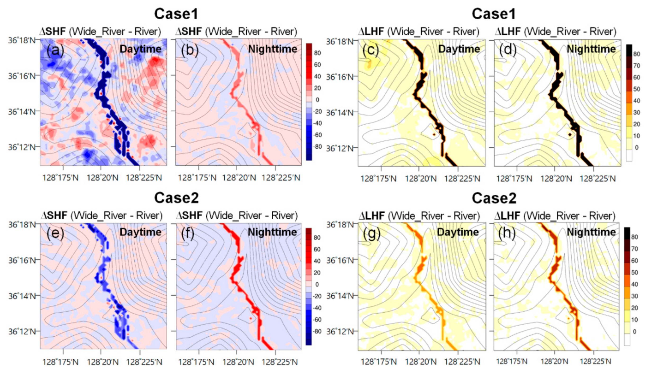
3.2. Changes of Meteorological Environment by Weir

Figure 5 shows mean differences between the Wide_River and River scenarios for Ta (∆Ta) and q (∆q) during the daytime (09:00~18:00 LST) and nighttime (19:00~06:00 LST) for Case1 and Case2.

In both cases ∆Ta, the highest difference in Ta indicated in areas, where the land was converted to water, with negative ∆Ta in daytime and positive ∆Ta at night. In Case1, the ∆Ta showed up to −2.5 °C for area with conversion from land to water and varied between −0.8 and 0.8 °C in the surroundings of the river in daytime (Figure 5a). The highest positive ∆Ta (2 °C) was shown in some areas changed from land to water at night. The expanded river caused an increase in Ta on the river and bank on the contrary to daytime, but the impact was notably weaker compared to daytime (Figure 5b). In Case2, the change amount of ∆Ta at daytime was smaller compared to nighttime (2 °C) in areas converted from land to river. The surroundings of the river showed a slight change in Ta between −0.2 and 0.2 °C in day and night (Figure 5e,f). It shows that the river increased its role as a cold source during the daytime and as a heat source during the nighttime. During the day, the land heats and during the night cools more rapidly than water mainly due to smaller heat capacity, and results in surface temperature difference between water and land during the day and night. Moreover, water bodies can mitigate temperature variation due to their evaporation [32]. It is consistent with the study by Oke [33], which shows that the high evaporation from water surface plays an important role in reducing the surrounding surface air temperature.

In the case of q, prevailing positive Δq in daytime proved that expanding the river can lead to increase in q, not only above water surface but also above surrounding land in both cases (Figure 5c,d,g,h). In Case1, the maximum Δq was 6 g kg⁻¹ during daytime and 1.4 g kg⁻¹ at night over the areas of modified LULC. In Case2, the distribution of ∆q revealed to be similar during day and night. In Case2, the distribution of ∆q revealed to be similar during day and night, in which maximum ∆q showed 0.6 g kg⁻¹ for area with conversion from land to water and the surroundings of the river varied ∆q between −0.2 and 0.2 g kg⁻¹. The ∆q is a variable along the major axis of the river, but it does not correlate to the elevation around the river nor with specific LULC type. It appears that the ∆q around the river was high at areas where a larger part of the land was converted to water, which expands the evaporation source.

The Ta and q changes can be explained as changes in the sensible heat flux (SHF) and latent heat flux (LHF), respectively. Mean differences between the Wide_River and River scenarios for SHF (∆SHF) and LHF (∆LHF) in daytime and nighttime of Case1 and Case2 are shown in Figure 6.

In both cases, the expanded river made a decrease (an increase) in SHF above areas which land was converted to water in daytime (nighttime); also, the ∆SHF changes were affected even in the surroundings of the river (Figure 6a,b,e,f). The negative ∆SHF in daytime showed maximum 400 W m⁻², and SHF at night increased up to 90 W m⁻² over the areas of modified LULC in Case1. In Case2, the change of ∆SHF was more pronounced at night than in the daytime. These SHF changes can explain the change of Ta that the negative ∆SHF leads to a decrease in daytime Ta and the positive ∆SHF makes an increase in nighttime Ta.

The LHF increased after river expansion, and the increase is greater in the area where the land has converted the water than surrounding the river in both cases (Figure 6c,d,g,h). The maximum ∆LHF in daytime (nighttime) was 280 W m⁻² (140 W m⁻²) in Case1, and the maximum ∆LHF in daytime (nighttime) was 30 W m⁻² (60 W m⁻²) in Case2. An increase in vapor sources caused by the expansion of the water surface leads to an increase in LHF that can explain an increase in the q. Although the increase in LHF was greater in nighttime than in the daytime, the increase in q was greater during the daytime in Case1. The atmosphere increases its capacity holding water vapor at high temperatures. Accordingly, the amount of the q increases as the LHF increases at near surface during the daytime. On the other hand, the q at night does not increase as much it does in the daytime, because condensation promptly occurs when the atmosphere becomes saturated above the open water surface. In the simulation, this leads to formation of liquid water content above the river during the night (not shown).

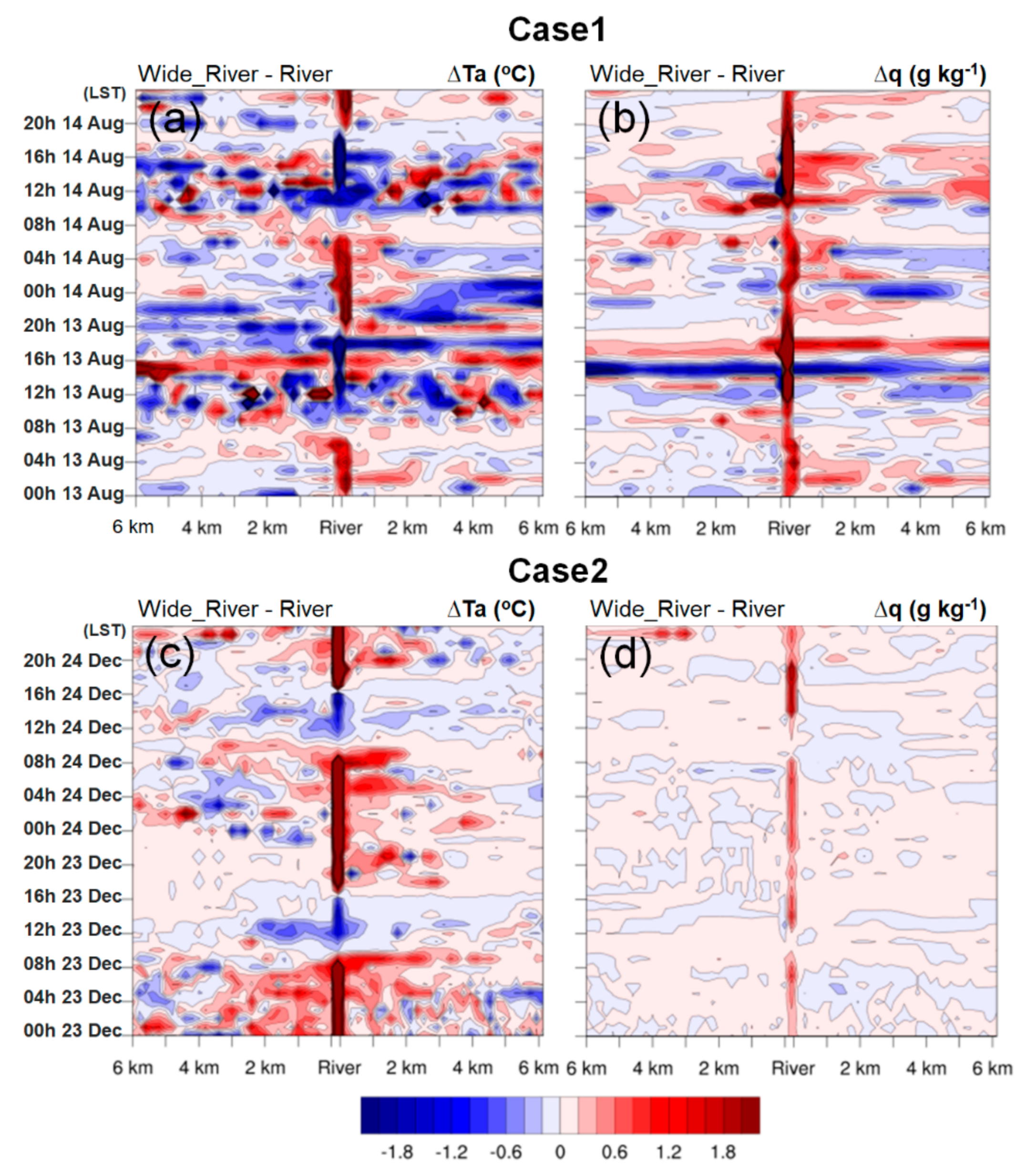
3.3. Range of Affected Area

A Hovmölller diagram and a paired t-test were used to investigate the distance from the river up to where the LULC change affected the meteorological fields in the simulation (hereafter “distance of affected area”). Rather than finding the absolute distance of potential impact, we estimate the relative distance to the magnitude of the impact.

Figure 7 presents the Hovmöller diagrams of the ∆Ta and ∆q with distance up to 6 km from the river (abscissa-axis) and time (ordinate-axis). The location of the cross section is indicated by the line between points A and B in Figure 2b.

The distance of the affected area of ∆Ta and ∆q varied with the time of day. In Case1, the distance of affected area of ∆Ta was relatively large during the daytime due to the significant ∆SHF (see Figure 6a) and strong wind conditions. The distribution of ∆Ta between 8:00 and 15:00 was horizontally inhomogeneous. In contrast, very homogeneous distributions of ∆Ta along abscissa-axis with a long distance of affected area and strong magnitude can be distinguished between 15:00 and 19:00, but only on 13 August. Surprisingly, the ∆Ta suddenly changed from positive to negative at 18:00 which corresponds to the time of shading effect onset due to local topography before the sunset. However, the distribution of ∆Ta between 15:00 and 19:00 in 14 August was different. ∆Ta was horizontally homogeneous but with a much weaker magnitude than in 13 August. During nighttime, the distance of affected area of ∆Ta was relatively small. The smallest distance of affected area was found in early mornings between 06:00 and 08:00, which can be related to calm wind conditions and small ∆SHF (see Figure 6b) during nights and early mornings. The ∆q in Case1 shows similar patterns as ∆Ta but with the opposite sign. The overall distribution of ∆q over the studied period was somehow more homogeneous than distribution of ∆Ta.

In contrast to Case1, in Case2 the distance of affected area of ∆Ta was largest in nighttime and smallest in daytime. This demonstrates the role of the river as a warming source in winter and a cooling source in summer. In Case2, ∆q shows very small variation with time, small magnitude and very short distance of affected area. The minimum effect of the river was found between 08:00 and 12:00 on 23 and 24 December, which corresponds with small ∆LHF in daytime (see Figure 6g).

The Hovmöller diagram is a convenient tool to investigate the change of affected area over the studied period but only for a specific cross-section of a region. To define a representative value of the distance of affected area, the paired t-test was applied. The method calculates the statistical significance of change in meteorological fields over the whole domain. The representative value was computed as the mean distance of the affected area along the major river axis considering both sides of river.

The distance of affected area at a single point of river was considered as a length of consecutive grid cells with statistically significant change (p < 0.05) from the point. Figure 8 and Figure 9 show the ∆Ta and ∆q for Case1 and Case2, respectively. The area with p < 0.05 was marked by red color.

The results of Case1 shown in Figure 8 revealed that most of the influence, in the regions with negative ∆Ta (indicated in Figure 5a), is statistically significant which proves the enhancement of the cooling effect by extending of the river width in summer, but the mean distance of affected area was only 234 m from the river. In nighttime the mean distance of significant warming effect of the wide river was even smaller (145 m) than in daytime. The mean distance of affected area by positive ∆q was larger, accounting for 341 m in daytime and 1059 m at night. Moreover, the east side of the river was continuously significant, caused by northwesterly winds at night (not shown).

The overall smallest mean distance of affected area was found to be 19 m in the negative ∆Ta in daytime of Case2 (Figure 9a). On the other hand, the largest mean distance of the affected area 1100 m belongs to the positive ∆Ta in nighttime of Case2 (Figure 9b) which proves the significant enhancement of the warming effect by extending of the river width in winter. The mean distance of the affected area with statistically significant positive ∆q was 527 m in daytime and 361 m in nighttime. The maximum and mean distances of the affected area from the river are summarized in

Table 2. Summary of the maximum and mean distances of the affected area from the river.

		Day		Night
		Max (m)	Mean (m)	Max (m)	Mean (m)
Case1	Air temperature	2000	234	1200	145
	Mixing ratio	2400	341	4000	1059
Case2	Air temperature	565	19	4600	1100
	Mixing ratio	3200	527	2600	361

.

4. Discussion

It is important to note that the numerical simulation in our study has several limitations. For example, we use uniform temporal and spatial distribution of Tw-based observational data in the simulation. The WRF model offers an option for initialization of inland Tw by interpolating the sea surface temperature over the land. However, we found this approach may produce a nontrivial error which in our study could have a significant impact on the results. Therefore, the initial Tw was set using the observed Tw average over the studied period, and, for simplicity, the Tw was kept temporally constant. Another approach would be to update the Tw during the simulation at a certain interval, however, from the time-series of observed Tw (Figure 3), it is evident that the temporal variation in Tw was minimal, especially during the winter experiment. The standard deviations during summer (Case1) and winter (Case2) experiments were only 0.97 and 0.23 °C, respectively. Therefore, in our study, the constant averaged value provides a sufficiently accurate representation of Tw. For longer simulations, we highly recommend considering the temporal variation of Tw and updating the Tw value during the simulation.

Another limitation was the spatial uniformity Tw. Since Tw was measured only at a single point in the center of the weir, the spatial variability during experiments was unknown. In contrast to lakes, rivers are generally well mixed dynamic systems with minimal temperature variation along the major axis of the river. Although, in the real world, a horizontal temperature gradient may exist across the riverbank depending on the water depth, to obtain such information, a high-resolution remote sensing technique might need to be applied. It is also worthy to note, that during the Gumi Weir construction project, the river floor was dredged into a trapezoidal shape with steep slopes, resulting in almost uniform depth across the river. To account for the temperature differences that may exist at very narrow areas near the edges of the river, the model would have to be deployed with an ultra-fine resolution grid (for example 10 m or less), which would be another technical challenge. Therefore, considering data availability and horizontal resolution of our model’s grid, the spatial gradient was negligible, and Tw was set to uniform over the whole water body.

Lastly, the simulations were conducted only for two case studies, which are sunny clear days with high solar radiation, and only a few meteorological variables were considered. A long-term simulation, covering whole seasons could provide more generalized information about the influence of LULC on local meteorological conditions. Moreover, adding additional variables such as wind speed and wind direction could clarify the influence of a weir construction on local circulation patterns.

5. Concluding Remarks

The impact of LULC change on near-surface weather variables due to a weir construction was investigated based on a high-resolution WRF model and the range in which the weather change that occurred was analyzed using a paired t-test. An extension of the river width by 300 m on average showed the change in weather variables of Ta, q, SHF, and LHF, not only over the water surface of the river but also over surrounding land near the river. The change in Ta showed to be proportional to the change in SHF, and the q was increased due to evaporation for the extended water surface with an increase in LHF for each case study. The results of the paired t-test revealed that a 1.5 times increase in width in the Nakdong river led to a noticeable change in Ta and q with mean distance of the affected area up to 1100 m from the river shores. The results of this study could offer an understanding of the effects of small weir construction on local weather changes.

References

1. Hohli, A.; Frenken, K. Evaporation from Artificial Lakes and Reservoirs; FAO-Aquastat: Rome, Italy, 2015; p. 10. [Google Scholar]
2. Hogeboom, R.J.; Knook, L.; Hoekstra, A.Y. The blue water footprint of the world’s artificial reservoirs for hydroelectricity, irrigation, residential and industrial water supply, flood protection, fishing and recreation. Adv. Water Resour. 2018, 113, 285–294. [Google Scholar] [CrossRef]
3. Lee, C.B. Changes of fog days and cloud amount by artificial lakes in Chuncheon. Asia-Pac. J. Atmos. Sci. 1981, 17, 18–26. [Google Scholar]
4. Hong, S.G. Increase of the fogs in Andong due to the construction of Andong reservoir. Asia-Pac. J. Atmos. Sci. 1982, 18, 26–32. [Google Scholar]
5. Stivari, S.M.; de Oliveira, A.P.; Karam, H.A.; Soares, J. Patterns of local circulation in the Itaipu Lake area: Numerical simulations of lake reeze. J. Appl. Meteorol. 2003, 42, 37–50. [Google Scholar] [CrossRef]
6. Policarpo, C.; Salgado, R.; Costa, M.J. Numerical Simulations of Fog Events in Southern Portugal. Adv. Meteorol. 2017, 2017, 1–16. [Google Scholar] [CrossRef]
7. Vogel, J.L.; Huff, F.A. Fog Effects Resulting from Power Plant Cooling Lakes. J. Appl. Meteorol. 1975, 14, 868–872. [Google Scholar] [CrossRef] [Green Version]
8. Brant, G.; Oliphant, A.J.; Blesius, L. Impacts of coastal advection fog on the surface radiation regime. AGUFM 2008, 2008, A51H-0206. [Google Scholar]
9. Bates, G.T.; Giorgi, F.; Hostetler, S.W. Toward the Simulation of the Effects of the Great Lakes on Regional Climate. Mon. Weather. Rev. 1993, 121, 1373–1387. [Google Scholar] [CrossRef]
10. Jeon, B.I.; Lee, Y.M. A change of local meteorological environment according to dam construction of Nakdong-River: II. Estimation using numerical model. J. Environ. Sci. 2002, 11, 281–288. [Google Scholar] [CrossRef]
11. Samuelsson, P.; Kourzeneva, E.; Mironov, D. The impact of lakes on the European climate as simulated by a regional climate model. Boreal Environ. Res. 2010, 15, 113–129. [Google Scholar]
12. Skamarock, W.C.; Klemp, J.B.; Dudhia, J.; Gill, D.O.; Barker, D.M.; Wang, W.; Powers, J.G. A Description of the Advanced Research WRF Version 2 (No. NCAR/TN-468+ STR). National Center for Atmospheric Research Boulder Co Mesoscale and Microscale Meteorology Div. 2005. Available online: https://apps.dtic.mil/dtic/tr/fulltext/u2/a487419.pdf (accessed on 9 December 2020).
13. Byon, J.-Y.; Choi, Y.-J.; Seo, B.-K. Numerical Simulation of Local Circulation over the Daechung Lake Area by Using the Mesoscale Model. J. Korean Earth Sci. Soc. 2009, 30, 464–477. [Google Scholar] [CrossRef]
14. Park, S.K.; Kim, J.H. A study on changes in local meteorological fields due to a change in land use in the lake Shihwa region using synthetic land cover data and high-resolution mesoscale model. Atmosphere 2011, 21, 405–414. [Google Scholar] [CrossRef]
15. Cao, Q.; Yu, D.; Georgescu, M.; Han, Z.; Wu, J. Impacts of land use and land cover change on regional climate: A case study in the agro-pastoral transitional zone of China. Environ. Res. Lett. 2015, 10, 124025. [Google Scholar] [CrossRef]
16. Yun, J.I.; Hwang, K.H.; Chung, H.H.; Shin, M.Y.; Lim, J.T.; Shin, J.C. Effects of an artificial lake on the local climate and the crop production in Suncheon area. Asia-Pac. J. Atmos. Sci. 1997, 33, 409–427. [Google Scholar]
17. Catalano, F.; Moeng, C.-H. Large-Eddy Simulation of the Daytime Boundary Layer in an Idealized Valley Using the Weather Research and Forecasting Numerical Model. Bound. Layer Meteorol. 2010, 137, 49–75. [Google Scholar] [CrossRef] [Green Version]
18. Moeng, C.-H.; Dudhia, J.; Klemp, J.; Sullivan, P. Examining Two-Way Grid Nesting for Large Eddy Simulation of the PBL Using the WRF Model. Mon. Weather Rev. 2007, 135, 2295–2311. [Google Scholar] [CrossRef]
19. Talbot, C.; Bou-Zeid, E.; Smith, J. Nested Mesoscale Large-Eddy Simulations with WRF: Performance in Real Test Cases. J. Hydrometeorol. 2012, 13, 1421–1441. [Google Scholar] [CrossRef]
20. Kang, M.; Lim, Y.-K.; Cho, C.; Kim, K.R.; Park, J.S.; Kim, B.-J. The Sensitivity Analyses of Initial Condition and Data Assimilation for a Fog Event using the Mesoscale Meteorological Model. J. Korean Earth Sci. Soc. 2015, 36, 567–579. [Google Scholar] [CrossRef]
21. Hong, S.-Y.; Noh, Y.; Dudhia, J. A New Vertical Diffusion Package with an Explicit Treatment of Entrainment Processes. Mon. Weather Rev. 2006, 134, 2318–2341. [Google Scholar] [CrossRef] [Green Version]
22. Pope, S.B. Turbulent Flows; Cambridge University Press: Cambridge, UK, 2000; p. 771. [Google Scholar]
23. Skamarock, W.C.; Klemp, J.B.; Dudhia, J. A Description of the Advanced Research WRF Version 3; NCAR Tech. Note NCAR/TN–4751 STR: Boulder, CO, USA, 2008; p. 113. [Google Scholar]
24. Walters, D.; Boutle, I.; Brooks, M.; Melvin, T.; Stratton, R.; Vosper, S.B.; Wells, H.; Williams, K.; Wood, N.; Allen, T.; et al. The Met Office Unified Model Global Atmosphere 6.0/6.1 and JULES Global Land 6.0/6.1 configurations. Geosci. Model Dev. 2017, 10, 1487–1520. [Google Scholar] [CrossRef] [Green Version]
25. Chen, F.; Dudhia, J. Coupling an advanced land surface-hydrology model with the Penn State-NCAR MM5 modeling system. Part I: Model implementation and sensitivity. Mon. Weather Rev. 2001, 129, 569–585. [Google Scholar] [CrossRef] [Green Version]
26. Lim, K.-S.S.; Hong, S.-Y. Development of an Effective Double-Moment Cloud Microphysics Scheme with Prognostic Cloud Condensation Nuclei (CCN) for Weather and Climate Models. Mon. Weather Rev. 2010, 138, 1587–1612. [Google Scholar] [CrossRef] [Green Version]
27. Mlawer, E.J.; Taubman, S.J.; Brown, P.D.; Iacono, M.J.; Clough, S.A. Radiative transfer for inhomogeneous atmospheres: RRTM, a validated correlated-k model for the longwave. J. Geophys. Res. Space Phys. 1997, 102, 16663–16682. [Google Scholar] [CrossRef] [Green Version]
28. Chou, M.D.; Suarez, M.J. An efficient thermal infrared radiation parameterization for use in general circulation models. NASA Tech. Memo 1994, 104606, 1–85. [Google Scholar]
29. Kang, J.H.; Suh, M.S.; Kwak, C.H. A Comparison of the Land Cover Data Sets over Asian Region: USGS, IGBP, and UMd. Atmosphere 2007, 17, 159–169. [Google Scholar]
30. Ministry of Environment. Available online: Egis.me.go.kr/map/map.do?type=land (accessed on 17 September 2019).
31. Wilks, D.S. Statistical Methods in the Atmospheric Sciences; Academic Press: Cambridge, MA, USA, 2011; Volume 100. [Google Scholar]
32. Sun, R.; Chen, L. How can urban water bodies be designed for climate adaptation? Landsc. Urban Plan. 2012, 105, 27–33. [Google Scholar] [CrossRef]
33. Oke, T.R. Boundary Layer Climates; Routledge: London, UK, 1987. [Google Scholar]
Figure 1. Maps of topography height of Domain1 and Domain2 which cover the area of Gumi Weir in the Nakdong River. Domain2 includes 6 Automatic Weather Stations (circles) and the measurement site of water surface temperature (triangle).
Atmosphere 11 01337 g001
Figure 2. LULC map before (a) and after (b) the construction of the Gumi Weir. LULC data have a 30m horizontal resolution from the Korean Ministry of Environment. An unfilled square is an analysis area, and line A–B is used for range analysis of weather variables change.
Atmosphere 11 01337 g002
Figure 3. Time series of observed air temperature, relative humidity, wind speed, wind direction, and water temperature for (a) Case1 (13 August 2013) and (b) Case2 (23 December 2013) at S1.
Atmosphere 11 01337 g003
Figure 4. Scatter plots of simulated and observed hourly air temperature at 2 m (a,c) and mixing ratio (b,d) at 2 m for Case1 (a,b) and Case2 (c,d) of the Wide_River scenario. Each variable has different scales on the x and y axis.
Atmosphere 11 01337 g004
Figure 5. Horizontal distribution of the mean differences between Wide_River and River (Wide River minus River) scenario for air temperature (ΔTa; a,b,e,f) and mixing ratio (Δq; c,d,g,h) at day (a,c,e,g) and night (b,d,f,h) for Case1 (ad) and Case2 (eh). The unfilled contours indicate a terrain height from 40 to 340 at intervals of 20.
Atmosphere 11 01337 g005
Figure 6. Horizontal distribution of the mean differences between Wide_River and River (Wide River minus River) scenario for sensible heat flux (ΔSHF; a,b,e,f) and latent heat flux (ΔLHF; c,d,g,h) at day (a,c,e,g) and night (b,d,f,h) for Case1 (ad) and Case2 (eh). The unfilled contours indicate a terrain height from 40 to 340 at intervals of 20. Also, different figure scales are used in the ΔSHF and ΔLHF.
Atmosphere 11 01337 g006
Figure 7. The Hovmöller diagram of the ΔTa (a,c) and Δq (b,d) with distance up to 6 km from the river (abscissa–axis) and time (ordinate–axis) for Case1 (c) and Case2 (d). The location of the cross section is indicated by the line between points A and B in Figure 2b.
Atmosphere 11 01337 g007
Figure 8. Horizontal distribution of a paired t-test result for ΔTa (a,b) and Δq (c,d) in daytime (a,c) and nighttime (b,d) for Case1. Area with significant change (p < 0.05) is marked in red, and the water area after weir construction is marked in blue.
Atmosphere 11 01337 g008
Figure 9. Horizontal distribution of a paired t-test result for ΔTa (a,b) and Δq (c,d) in daytime (a,c) and nighttime (b,d) for Case2. Area with significant change (p < 0.05) is marked in red, and the water area after weir construction is marked in blue.
Atmosphere 11 01337 g009