Multifractal Cross Correlation Analysis of Agro-Meteorological Datasets (Including Reference Evapotranspiration) of California, United States

Abstract

The multifractal properties of six acknowledged agro-meteorological parameters, such as reference evapotranspiration (ET0), wind speed (U), incoming solar radiation (SR), air temperature (T), air pressure (P), and relative air humidity (RH) of five stations in California, USA were examined. The investigation of multifractality of datasets from stations with differing terrain conditions using the Multifractal Detrended Fluctuation Analysis (MFDFA) showed the existence of a long-term persistence and multifractality irrespective of the location. The scaling exponents of SR and T time series are found to be higher for stations with higher altitudes. Subsequently, this study proposed using the novel multifractal cross correlation (MFCCA) method to examine the multiscale-multifractal correlations properties between ET0 and other investigated variables. The MFCCA could successfully capture the scale dependent association of different variables and the dynamics in the nature of their associations from weekly to inter-annual time scales. The multifractal exponents of P and U are consistently lower than the exponents of ET0, irrespective of station location. This study found that joint scaling exponent was nearly the average of scaling exponents of individual series in different pairs of variables. Additionally, the α-values of joint multifractal spectrum were lower than the α values of both of the individual spectra, validating two universal properties in the MFCCA studies for agro-meteorological time series. The temporal evolution of cross-correlation determined by the MFCCA successfully captured the dynamics in the nature of associations in the P-ET0 link.

1. Introduction

Characterization of agro-meteorological time series is a major concern for irrigation and water resource planners. Agro-meteorological time series often possess non-linear, non-stationary and complex temporal scaling characteristics [1], which make the accurate prediction of their course difficult. Any improved understanding on the fluctuations and scaling characteristics of such time series may enhance the modeling efforts aimed at a fuller understanding of their structures. Many of agro-meteorological time series possesses multiple time scales ranging from sub-daily to yearly, in which the turbulence induces stochastic fluctuations at smaller scales, whereas the complex nonlinear interactions between variables induce fluctuations at larger scales. The atmospheric turbulence plays a key role in the scaling behavior of the agro-meteorological time series. The atmospheric turbulence in the inertial range can be statistically described by scale invariant processes, due to the fundamental symmetries of the Navier-Stokes equations [2]. The scale invariant processes do not have any characteristic scale over the scaling range, the energy fluxes may be conserved from a large to a small-scale and the interactions occur mainly between neighboring scales. This can lead to a cascade process, which is generally described as eddies breaking up into smaller sub-eddies, each of which receives a part of the flux of its parent body [3]. Fractals, a term coined by Benoit Mandelbrot, can be considered as a rough or fragmented geometric shape that can be subdivided in parts, each of which is (at least approximately) a reduced-size copy of the whole [4]. Many of the complex agro-meteorological time series often exhibit self-similarity or self-affinity and scale invariance over certain range of time scales which are typical characteristics of fractals. Thus the analogy of such signals with the stochastic cascade models in fully developed turbulence can lead to fractal behavior in them. To illustrate the above stated cascade phenomenon of flux transfer, the classical Kolmogorov and Corrsin-Obukhov scaling laws were proposed [5,6,7,8] which later on routed the determination fractal behavior of time series. But in many of the atmospheric variables, the scale by scale flux transfer need not be homogenous, instead it may be intermittent [9,10]. To address such issues the alternate scaling cascade models were proposed [11,12,13]. In short, such turbulence models were adapted to reproduce scale invariance properties through the use of fractal geometry and more on theoretical foundations of this issue can be found in literature [14,15,16].

The detailed conceptual framework on fractal behavior of time series was provided by Mandelbrot [4] and later on different methods were proposed to determine the fractal characteristics of the time series. The long-range dependency is closely related to the scaling property and fractality of the time series, as was noticed by Hurst [17], one of the earlier contributors in this field. The fractal property of the time-series is strongly associated with its persistence as the fractal dimension (D) and Hurst exponent (H) can be related to each other as D = 2–H [18]. A value of H between 0.5 and 1 indicates a series as long-term power law correlated and that between 0 and 0.5 indicates that the series is short term correlated. There are numerous methods to determine the fractal dimension or Hurst exponent of the time series including the classical Structure Function Analysis, Rescaled Range (R/S) method and Fourier spectrum [19,20]. However, later on it was found that a single fractal dimension was not sufficient to describe the whole phenomenon and many sophisticated models were proposed based on multifractal formalism since 1980 [21,22,23,24,25,26]. Hence, based on multifractal theory also Hurst exponent can be evaluated and the value of scaling exponent for the second order statistical moment is widely recognized as similar to the classical Hurst exponent by many researchers [27].

Multifractal Detrended Fluctuation analysis (MFDFA) propounded by Kantelhardt et al. [24], is one of the most popular approaches for the multifractal characterization of time series. The method was extensively applied for different hydrological like streamflow [28,29,30,31], meteorological time series such as rainfall, drought index, temperature, solar radiation and relative air humidity [32,33,34,35,36,37,38,39,40,41,42,43]. Even though some alternative methods like joint-multifractal analysis was proposed recently for the multifractal characterization of reference evapotranspiration (ET0) time series [35], no comprehensive study of global recognition was reported for the characterization of ET0 time series employing MFDFA and its extended cross correlation variants. One of the essential components for irrigation water management is the evapotranspiration (ET). ET is the simultaneous process of transfer of water to the atmosphere by transpiration and evaporation in a soil–plant system and its quantification is to be preceded by the estimation of reference evapotranspiration. ET0 has been defined as the rate of evapotranspiration from an extensive grassed area of 8–15 cm tall, uniform, actively growing, completely shading the ground and with adequate water [44]. Later on, Allen et al. [45] elaborated on the concept of ET0, by referring it to an ideal 12 cm high crop with a fixed surface resistance of 70 SD⁻¹ and an albedo of 0.23. Different meteorological variables influence the estimation of ET0 and they were considered as potential inputs for modeling of ET0 [46]. Numerous modeling practices ranging from conventional statistical approaches to hybrid decomposition algorithms and data driven techniques were proposed to model ET0 [47,48,49,50,51]. The complex structure of ET0 and other agro-meteorological variables makes the accurate modelling a challenging task. Therefore, any efforts for exploring alternative modeling practices which can contribute towards improving the accuracy in predictions of such variables are appreciable. Fractal or multifractal modeling is another promising approach which can be adopted for modeling complex systems, for which the characterization of such time series is an essential prerequisite to proceed with such modeling practices. Understanding the inherent features of different time-series and their lagged influence have vital role in the accuracy of modeling ET0 and other time series following different alternative approaches. Fractal signatures are such features which can disseminate proper knowledge on the predictability and complexity of the time-series, which may eventually help in accurate modeling of agro-meteorological time series. Multifractal modeling is one potential alternative modeling approach and proper understanding of the persistence and multifractal properties is to be determined a priori before proceeding with such modeling. Moreover, the multifractal properties of time series may distinctly differ depending on terrain conditions. Understanding such differences in multifractal properties from stations of diverse terrain conditions may provide necessary scientific insights to find the reason behind such variability.

The determination of fractal behavior basically involves the determination of whether the fluctuations of the time series decrease with the increase in scale, following a power law relationship with an exponent such as F(s)~s^H, or not. In that case, the data is said to be scaling in that range i.e., there exists a certain degree of statistical scale-invariance. Persistence can be defined as the existence of some statistical dependence among successive values of the same variable, or among successive occurrences of a given event [52]. The fractal theory quantifies the diminishing nature of correlations (dependence), the autocorrelation function declines as a power-law. Thus, the persistence properties of hydro-meteorological signals can give useful insights into the autocorrelation structure of the time-series [53], which in turn may help in predictor selection in time-series approach for modeling of the agro-meteorological variables.

An appropriate selection of the predictor variables is an important step for the reliable prediction of ET0 using statistical or data-driven methods. The variables like solar radiation, temperature, wind speed, relative air humidity, etc., were reported to be appropriate inputs for the prediction of ET0 [46]. All these time series possess multiscaling behavior and advanced multiscale spectral analysis procedures, such as Wavelet transform or Hilbert Huang Transform (HHT) are helpful for investigating the mutual association between these variables [54]. The determination of Pearson correlation is the typical procedure in the estimation of possible dependency between the two candidate variables even in such multiscale approaches. However, some studies reported that Pearson correlation estimation may not be robust and can be misleading if outliers are present, as in the real-world data characterized by a high degree of non-linearity and non-stationarity [55]. In this context, estimating the scale dependent link in a multifractal perspective may give a realistic estimate for such studies. Podobnik and Stanley [56] proposed the detrended cross-correlation analysis (DCCA), to investigate power-law cross correlations between two candidate non-stationarity time series in a multifractal framework. Multifractal extension of DCCA (namely MFDCCA) and its variant namely Multifractal Detrending Moving Average Cross Correlation Analysis (MFXDMA) was also proposed by researchers [57,58]. Later on Oświecimka et al. [59] propounded a more generalized version of cross correlation analysis namely Multifractal Cross Correlation Analysis (MFCCA) which can also incorporate the sign of fluctuation function to their generalized moments [60,61]. DCCA and the above stated variants were used successfully for investigating the power law cross-correlations between different pairs of hydrological and meteorological datasets [62,63,64,65,66,67,68,69]. It is expected that understanding the scale dependent relationship between the predictor variables will eventually help for developing hybrid decomposition models for prediction of complex time series dataset [50]. Also such multiscale investigation may help in providing insights to the physical processes and the role of different meteorological variables behind ET0. In this context, the determination of correlation between different causal meteorological variables with ET0 is of great significance in agro-meteorological modeling. However, such associations were never investigated in the past in a multiscale-multifractal perspective.

Therefore, the specific objectives of this work include: (i) to investigate the multifractal properties of ET0 and meteorological variables like wind speed, air pressure, solar radiation, air temperature, relative air humidity at five stations located at distinctly different terrain conditions in California, USA; (ii) to investigate the power law correlations of different meteorological variables with ET0 using the novel MFCCA approach. The next section presents the theoretical details of MFDFA and MFCCA methods. The details of data used in the study are presented in the section thereafter. Subsequently, results of MF analysis and MFCC are presented along with relevant discussions. The major conclusions drawn from the study are presented in the last section.

2. Materials and Methods

In this study, firstly MFDFA method is applied to examine the multifractality of different agro-meteorological time series of California. Subsequently, MFCCA method is used to investigate the mutual association of different contributory meteorological variables with ET0. As the nonlinear properties (i.e., the long-term volatility correlations and the width of the multifractal spectrum) are strongly affected by the periodicities in agro-meteorological time series, the periodic seasonal trends in all the studied time series have to be filtered out. To remove them, the Seasonal and Trend decomposition using Loess (STL) method developed by Cleveland et al. [70] was used before performing the MFDFA and MFCCA analyzes.

2.1. MFDFA Method

The different steps of MFDFA are:

(1)

Determine the accumulated deviation of the time series signal X (x1, x2… xL) from its mean (so called ‘profile’) as:

$$P(i)={\displaystyle \sum _{k=1}^i\left[x_k-\overline{x}\right]}$$

(1)

where i = 1, 2,..., L, with mean $\overline{x}$ and length L.

(2)

Identify different independent sub-series of different lengths (called scale s) both in forward and backward directions.

(3)

Fit polynomial to each sub-series and find the difference between original sub-series and its fitted polynomial as:

$$f^2(s,\upsilon )=\frac{1}{s}{{\displaystyle \sum _{i=1}^s\left\{P[(\upsilon -1)s+i]-y_{\upsilon }(i)\right\}}}^2\mathrm{for}\upsilon =1,2,\dots ,N$$

(2)

and:

$$f^2(s,\upsilon )=\frac{1}{s}{{\displaystyle \sum _{i=1}^s\left\{P[L-(\upsilon -N)s+i]-y_{\upsilon }(i)\right\}}}^2\mathrm{for}\upsilon =N+1,\dots ,2N.$$

(3)

Here y_υ(i) is the polynomial used for fitting in fragment υ.

(4)

Determine the fluctuation function (FF) for different combination of scale s and statistical moment order q, based on step 3:

$$F{F}_q(s)={\left\{\frac{1}{2N}{\displaystyle \sum _{\upsilon =1}^{2N}{\left[f^2(s,\upsilon )\right]}^{q/2}}\right\}}^{1/q}$$

(4)

(5)

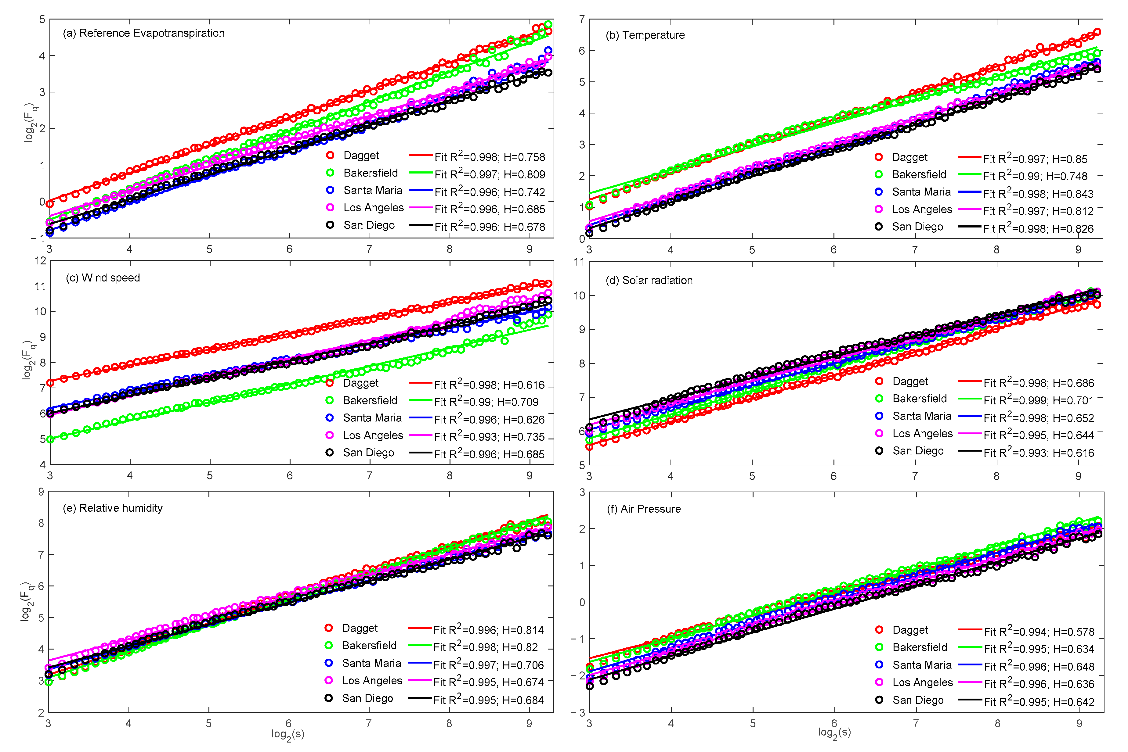
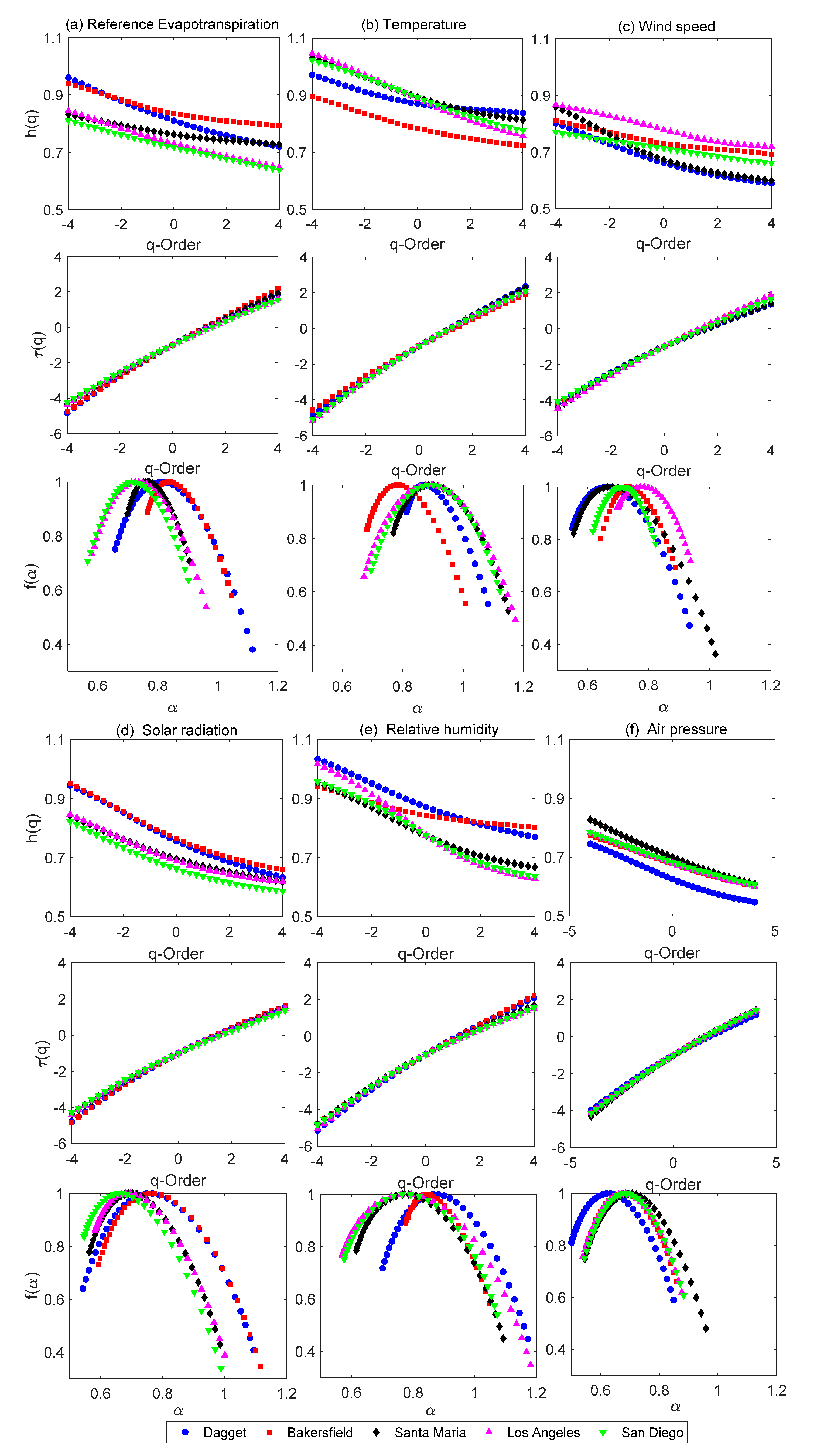
Develop the log-log plot of fluctuation function FF_q(s) vs. scale s. The slope of logarithmic plot of FF versus s is called generalized Hurst exponent (GHE) h(q) for different moment order q. The non-linear behavior of the plot between h(q) and q indicates the multifractality of the time series. For monofractal time series h(q) is independent of q. Multifractal behavior (a significant dependence of h(q) on q) will manifest itself only if small and large fluctuations scale differently in the time series. For positive values of q, h(q) describes the scaling behavior of the segments with large fluctuations, whereas for negative values of q, the scaling behavior of the segments with small fluctuations is described. While the precision of h(q) estimation depends mostly on the length of the time series, for large negative values of q (very small fluctuations) the precision of measurement is also starting to play a role. A detailed analysis on the precision of h(q) estimation for the MFDFA method was performed by López and Contreras [71]. The GHE value for q = 2 is considered to be equivalent to the classical Hurst exponent (H) [27,28]. From h(q) other useful exponents like mass exponent τ(q) or singularity exponent f(α) can be derived as follows:

$$\tau (q)=qh(q)-1$$

(5)

$$\alpha =\frac{d\tau (q)}{dq}$$

(6)

$$f(\alpha )=q\alpha -\tau (q)$$

(7)

The plot of f(α) vs. α is called as singularity spectrum, which will be inverted parabolic in shape with apex at unity for multifractal series. The base width of the spectrum (w = α_max − α_min) is an indicative of the strength of the multifractality in such a way that larger width indicates higher multifractal strength and vice versa. The symmetry of the spectrum (symmetric, left or right-skewed) indicates the dominancy for high (or low) fluctuations. It is quantified by a parameter called asymmetry index (AI), computed based on the width of right and left wings of the parabola as:

$$AI=\frac{\Delta {\alpha }_{left}-\Delta {\alpha }_{right}}{\Delta {\alpha }_{left}+\Delta {\alpha }_{right}}$$

(8)

with ∆α_left = α₀ − α_min and ∆α_right = α_max − α₀, respectively. If AI is zero, the spectrum is symmetric, positive values indicates a right skewed and negative values indicates a left-skewed spectrum. Negative values of AI suggest the existence of complex structures at the level of large fluctuation amplitudes in the respective series; they also suggest that the time series are characterized by a multifractal structure, which is insensitive to local fluctuations with small amplitudes. This means that a low weight can be attributed to low fractal exponents, which in turn suggests the frequent occurrence of extreme events [72]. The value of α at q = 0 (indicated as α₀ and called as Holder exponent) infers the complexity of the time series. The mathematical expressions for the computation of multifractal properties and the guidelines for selection of algorithm specific control parameters such as polynomial order, range of moment order, scaling range (s_min − s_max) etc. can be can be found in literature [73].

2.2. MFCCA Method

The different steps of MFCCA computational procedure can be described as follows:

(1)

For two time series x_i and y_i (I = 1, 2,…, N), determine the profiles as:

$$P_x(j)={\displaystyle \sum _{i=1}^j\left[x_i-\overline{x}\right]}$$

(9)

and:

$$P_y(j)={\displaystyle \sum _{i=1}^j\left[y_i-\overline{y}\right]}$$

(10)

where j = 1, 2,…, N and $\overline{x}$ and $\overline{y}$ are the mean of the two time series x_i and y_i.

(2)

Divide each profile P_x(j) and P_y(j) into N_s non-overlapping segments both in progressive and retrograde directions, to avoid any omission of time series data from the head or tail end of the series.

(3)

For each 2N_s segments, compute local trend of both “profiles” P_x(j) and P_y(j) by fitting polynomials p_X,υ^m(j) and p_Y,υ^m(j) of appropriate order m. The subtraction of the fitted polynomial from the original segment gives the covariance as given below:

$${{\phi }_{XY}}^2(\upsilon ,s)=\frac{1}{s}{\displaystyle \sum _{k=i}^s\left\{\left[P_x((\upsilon -1)s+k)-{p_{X,\upsilon }}^m(k)\right]\times \left[P_y((\upsilon -1)s+k)-{p_{Y,\upsilon }}^m(k)\right]\right\}}$$

(11)

where s is the length of υ segment.

(4)

Calculate detrended covariance by summation over all segments:

$${F^q}_{XY}(s)=\frac{1}{2N_s}{\displaystyle \sum _{\upsilon =0}^{2N_s-1}sign\left[{{\phi }_{XY}}^2(\upsilon ,s)\right]}{\left|{{\phi }_{XY}}^2(\upsilon ,s)\right|}^{q/2}$$

(12)

(5)

Check if F^q_XY(s) behaves as a power-law function of s (the scaling behavior), where s is the segmental sample size:

$${\left\{{F^q}_{XY}\left(s\right)\right\}}^{1/q}=F_{XY}\left(s\right)~s^{{\lambda }_{XY}\left(q\right)}.$$

(13)

The scaling exponent λ_XY(q) is similar to the generalized Hurst exponent h(q) in MFDFA and it can be obtained by observing the slope of log-log plot of F(s) versus s by ordinary least squares. The ratio between the detrended covariance function F^q_XY(s) obtained from MFCCA and the detrended variance functions F^q_X(s) and F^q_Y(s) obtained from MFDFA defines the detrended cross correlation ρ_XY(s) as:

$${\rho }_{XY}(s)=\frac{F_{XY}\left(s\right)}{\sqrt{F_X\left(s\right)F_Y\left(s\right)}}$$

(14)

Theoretically, the value of ρ_XY(s) ranges between −1 ≤ ρ_XY(s) ≤ 1. The MFCCA analysis facilitate the estimation of scale dependent correlation between two candidate time series, which can provide better insight into the physical association between the variables.

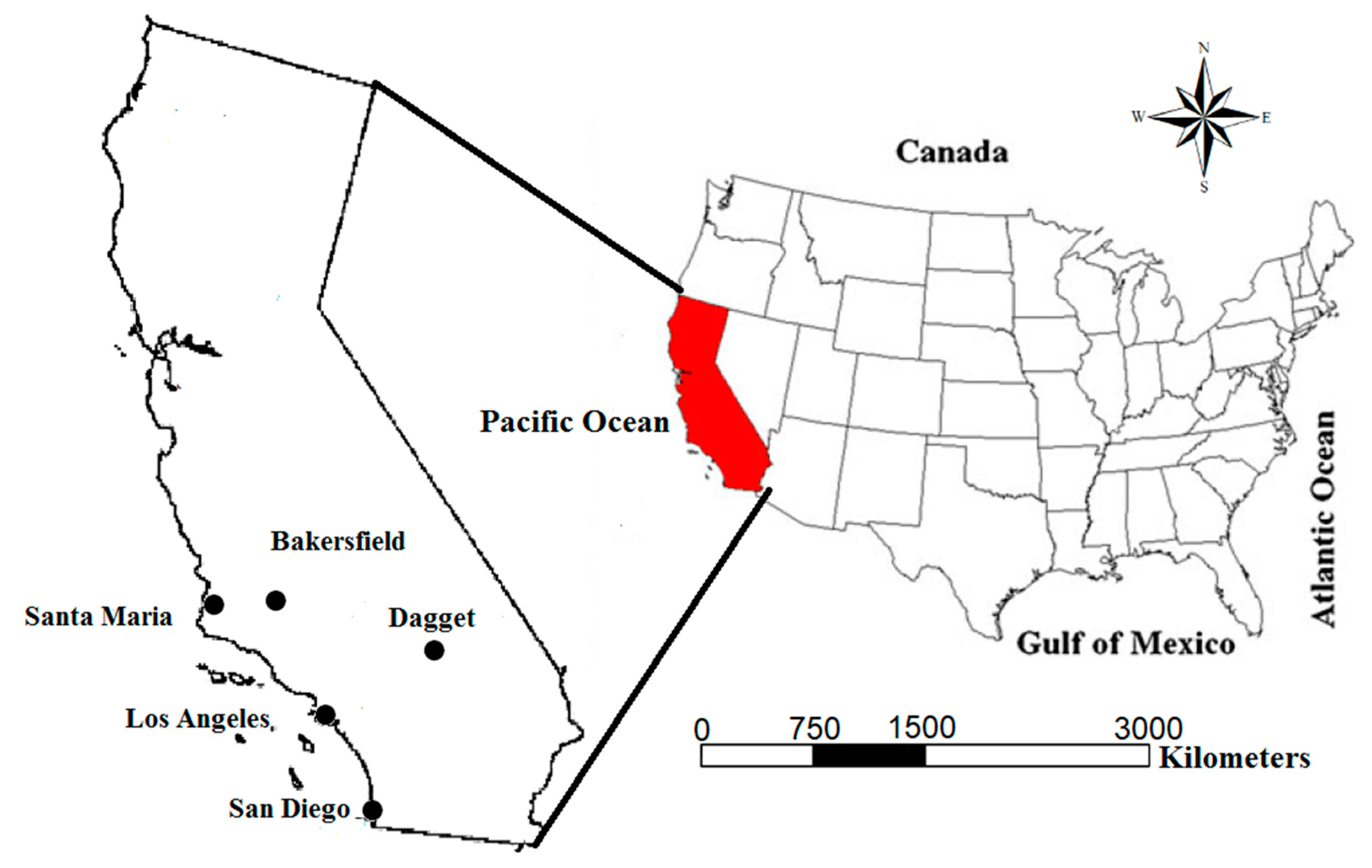
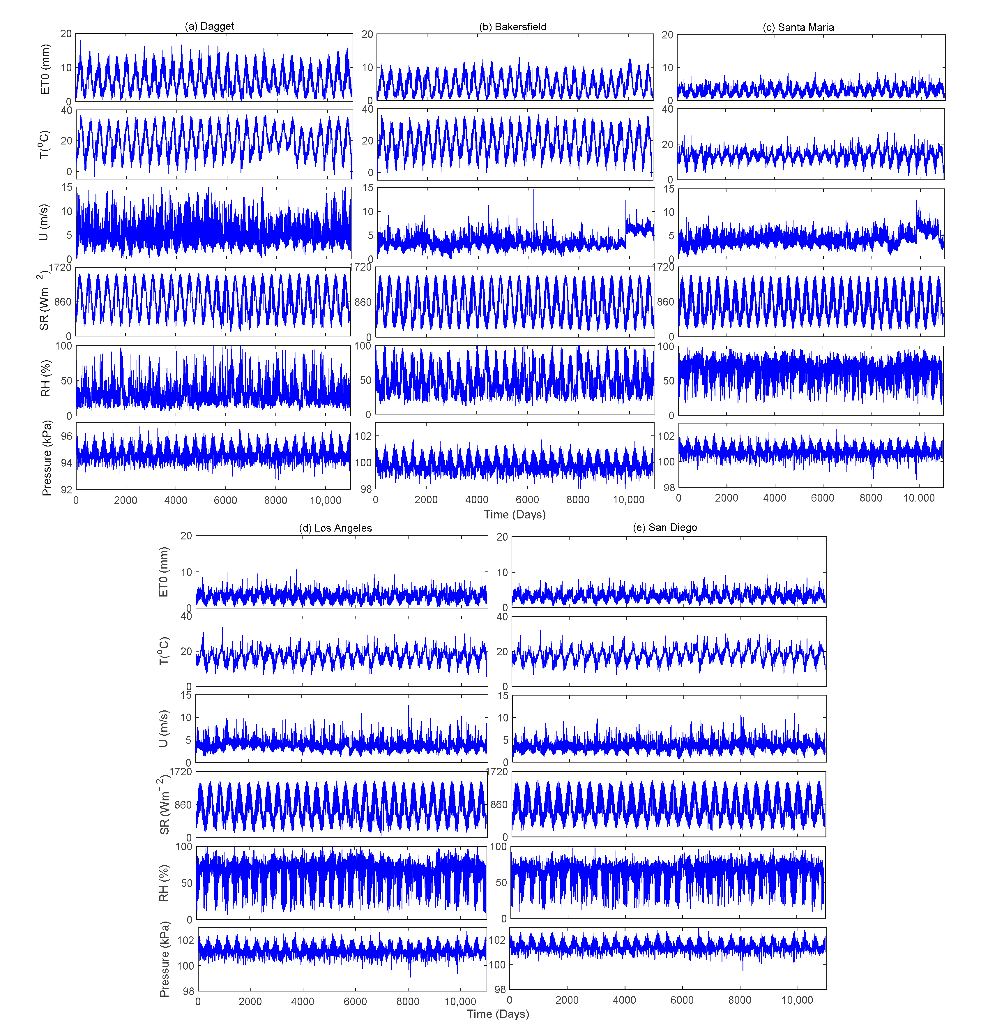
2.3. Study Area and Data

The multifractal characteristics of time series changes with latitude, altitude and distance from the coast [74]. Therefore, it is better to consider datasets from different terrain conditions and elevations. Considering this, the daily data of five automated weather stations of California, USA, namely Dagget (latitude 34.52° N, longitude 116.47° W), Bakersfield (35.26° N, 119.03° W), Santa Maria (34.96° N, 120.42° W), Los Angeles (34.02° N, 118.29° W), and San Diego (36.78° N, 119.72° W), operated by the United States Environmental Protection Agency (US EPA), were used in the study. The State of California extends along the shore of the Pacific Ocean between latitudes 32.5 and 42° N. Its more than 2100 km of coastline constitutes nearly three-fourths of the Pacific coastline of the conterminous United States. Los Angeles lies in a basin in Southern California adjacent to the Pacific Ocean and the city is the largest one in California. The average elevation of the city is only about 30 m above m.s.l. Los Angeles is a hot-summer Mediterranean climate as per Köppen Climate Classification (KCC) system [75], with hot, dry summers, and cooler wetter winters with lesser precipitation than typical Mediterranean climate. All the stations considered are located at radial distances within 180–250 km from the city of Los Angeles. Dagget city is located at north-east of Los Angeles by 200 km at the interior part of Southern California with no oceanic proximity. According to the KCC, Daggett has a semi-arid climate. There is very little rainfall year-round and diurnal temperature variation is high. In the winter, nights are often very cold while days are mildly cool. Meanwhile, summer nights are mildly warm while days can be extremely hot. The major land resource areas of the Daggett are Sonoran Basin and Range (Arizona, California, and Nevada, western range and irrigated region). The evaporation losses in Daggett site are moderately high due to the high temperature. The Bakersfield station is 180 km to the north of Los Angeles, situated in the center of Kern County, located in the extreme southern end of the Great San Joaquin Valley, and is partially surrounded by a horseshoe-shaped rim of mountains. The climate in Bakersfield has a hot desert type climate with very hot, dry summers, and winters that consist of mild days with chilly/cold nights. San Diego, with approximate height of 4 m above m.s.l., is located about 200 km to the south of Los Angeles on the coast of Pacific ocean. The basic climate is typical Mediterranean as per KCC with hot, sunny, and dry summers, and cooler, wetter winters. However, the city is much more arid, and winters are still dry on comparing with most other zones with this type of climate. The wet winter season of San Diego is influenced by the El Nino Southern Oscillation (ENSO) and it receives more winter storms with warmer and more humid conditions. During the La Nina phase, San Diego becomes drier with cooler and less humid conditions. Santa Maria is located in the central coast of California in the northern Santa Barbara county. It is approximately over 240 km north west of Los Angeles. The region experiences a cool Mediterranean climate (KCC typical of coastal areas of California north of Point Conception). The climate is mostly sunny, refreshed by the ocean breeze. The attitudes of these stations are 586, 151, 77, 30 and 4 m from the mean sea level, respectively. This helped to capture the differences in multifractal behavior with the altitudinal differences. Long daily records of air temperature (T), solar radiation (SR), wind speed (U), air pressure (P), relative air humidity (RH), and reference evapotranspiration (ET0) of 1961–1990 period are used for multifractal analysis. FAO−56 Penman–Monteith equation was used by United States Environmental Protection Agency for the estimation of ET0. The map showing locations of different stations is provided in Figure 1.

The measured daily climatic data for these stations were downloaded from the US EPA web server [76]. The respective time series are plotted in Figure 2. The quality control is a major prerequisite for using meteorological information, so it is highly necessary to ensure that the record structure of the data is correct and complete before proceeding with modeling of any time series and there are definite procedures to perform the quality control of the datasets [77,78,79].

However, in this case, the network is highly sophisticated and data was published by USEPA after rigorous quality examinations and used widely by other researchers [48,80]. However, along with the visual examination the data was checked for their continuity and also the chances of outliers was examined. No such anomalous observations and their replacement were needed and separate homogeneity analysis was not warranted in this case. The basic statistical parameters of the different datasets are provided in

Table 1. Statistical properties of the agro-meteorological datasets of California.

Station	Variable	Maximum	Minimum	Mean	Standard Deviation
Dagget	ET0 (mm)	18	0.2	6.42	3.37
	T (°C)	37.2	−5.3	19.72	8.47
	U (m/s)	15.973	0.174	5.04	2.22
	SR (Wm−2)	1576.2	102	993.9	359.5
	RH (%)	100	7	30.20	14.29
	P (kPa)	96.7	92.7	94.66	0.48
Bakersfield	ET0 (mm)	13	0.2	4.68	2.78
	T (°C)	37	−2.8	18.58	8.04
	U (m/s)	14.564	0	3.49	1.32
	SR (Wm−2)	1521.3	129.6	895.3	400.7
	RH (%)	100	12	48.10	18.56
	P (kPa)	101.7	97.7	99.83	0.50
Santa Maria	ET0 (mm)	10.6	0.3	3.21	1.22
	T (°C)	33.3	5.7	16.72	3.36
	U (m/s)	12.719	1.257	3.77	1.00
	SR (Wm−2)	1492.7	49.6	850.7	327.4
	RH (%)	100	7	65.22	16.07
	P (kPa)	103	99.1	101.19	0.37
Los Angeles	ET0 (mm)	9	0.5	3.03	1.21
	T (°C)	26.7	0.5	13.35	2.80
	U (m/s)	12.53	0.453	4.07	1.31
	SR (Wm−2)	1527.7	157.2	889.6	346.7
	RH (%)	98	16	65.34	13.78
	P (kPa)	102.5	98.6	100.80	0.38
San Diego	ET0 (mm)	9.4	0.5	3.31	1.18
	T (°C)	32.2	6.7	17.55	3.43
	U (m/s)	10.897	0.697	3.55	0.99
	SR (Wm−2)	1488.5	156.8	864.5	314.1
	RH (%)	100	10	63.99	14.02
	P (kPa)	103.1	99.5	101.46	0.35

.

3. Results and Discussion

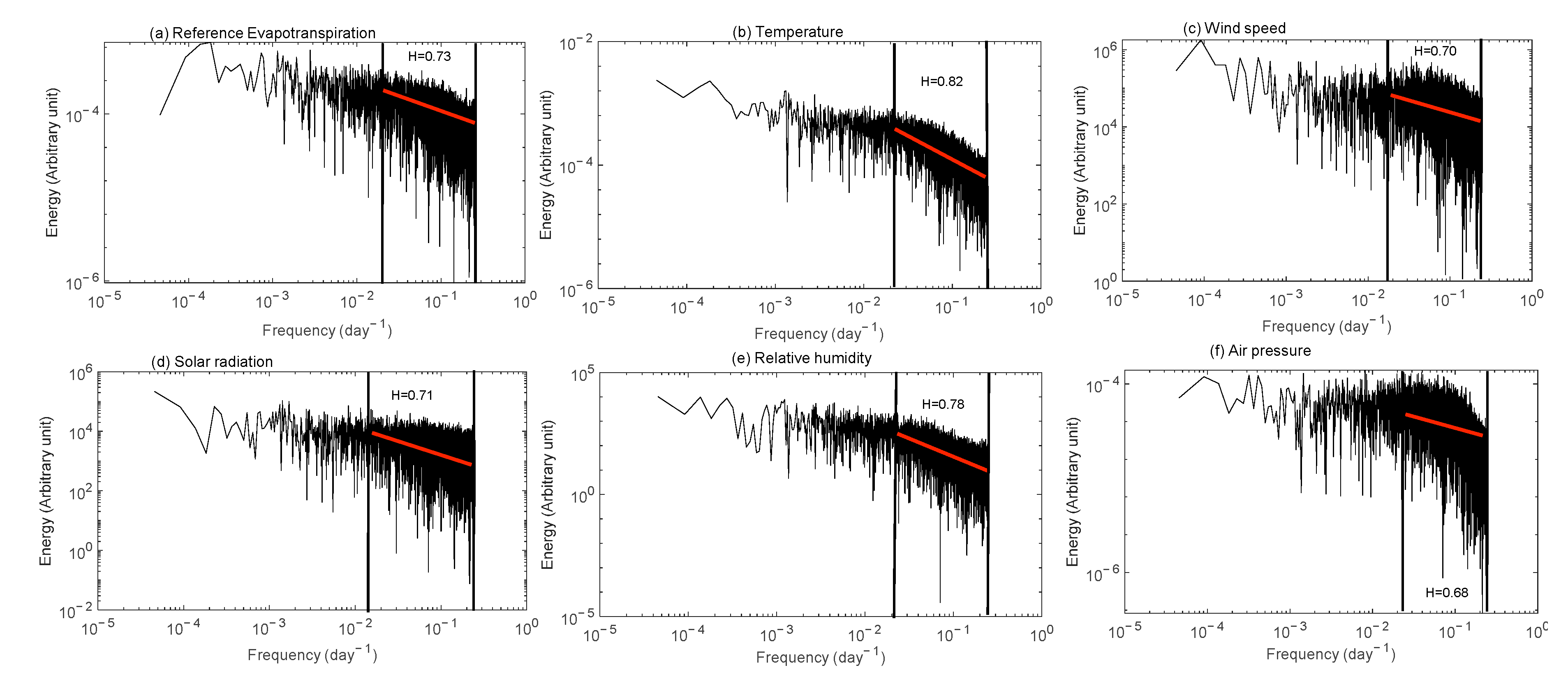
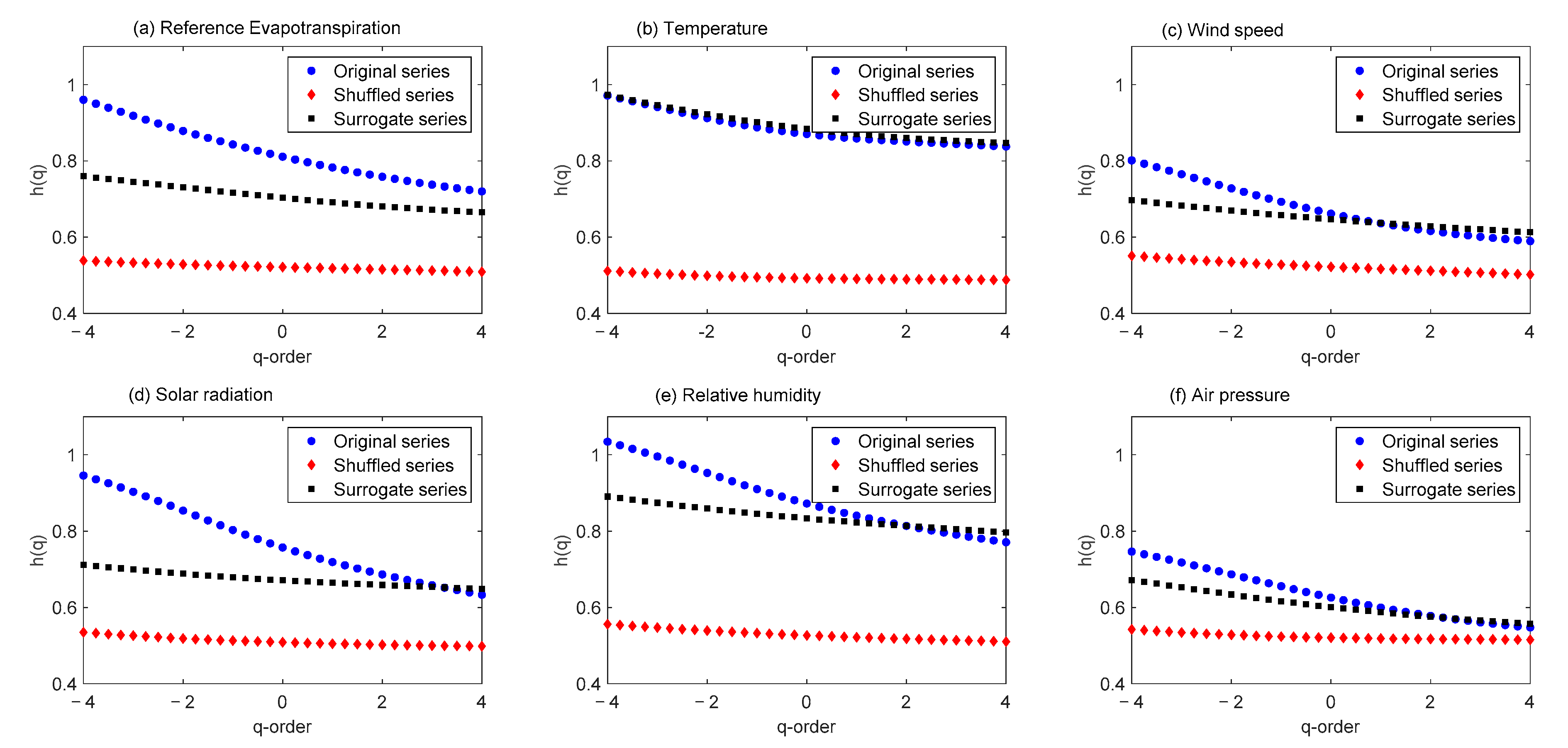
3.1. MFDFA of Agro-Meteorological Time Series

The multifractality of the five contributing time series (T, U, SR, RH, P) and ET0 time series of all the five stations were examined using MFDFA method. The minimum and maximum scale ranges can be fixed appropriately by following the guidelines stated in literature [72,73]. The minimum scale s_min greater than (m + 2), where ‘m’ is the polynomial order, is a widely accepted thumb rule. The maximum scale s_max is suggested to be chosen as up to L/10 [27]. Here, a rigorous trial and error exercise is made in the selection of the scale range considering the physics of the problem. The fluctuation functions are developed by considering the statistical moment orders from −4 to 4 are fixed and the first order polynomial (m = 1) was chosen for invoking MFDFA [41]. The fitting is considered to be acceptable on getting an R² ≥ 0.98 [81]. Thus a scaling range of [8:600] days was found to be appropriate to capture the scaling behavior, which corresponds from weekly to inter-annual period.

Different graphical representations such as GHE plot, mass exponent plot, multifractal spectrum were developed for all the six time series of each station and they are presented Figure 3. From these plots, the important multifractal parameters (H, W, AI, ∆h(q), ∆f(α) and α₀) were estimated and the values were provided in

Table 2. Multifractal parameters of agro-meteorological datasets of California.

Variable	Multifractal Properties
	H	W	AI	∆f(α)	∆h(q)	α0
Dagget
ET0	0.758	0.458	0.362	0.370	0.240	0.804
T	0.851	0.270	0.596	0.344	0.133	0.867
U	0.616	0.383	0.454	0.371	0.212	0.655
SR	0.687	0.551	0.260	0.232	0.313	0.747
RH	0.814	0.472	0.308	0.271	0.264	0.864
P	0.578	0.348	0.320	0.223	0.199	0.619
Bakersfield
ET0	0.810	0.279	0.529	0.307	0.147	0.831
T	0.748	0.325	0.403	0.275	0.173	0.778
U	0.710	0.246	0.300	0.109	0.120	0.728
SR	0.701	0.523	0.377	0.385	0.293	0.755
RH	0.820	0.269	0.527	0.305	0.138	0.840
P	0.634	0.309	0.210	0.132	0.172	0.672
Santa Maria
ET0	0.742	0.207	0.411	0.176	0.105	0.759
T	0.843	0.381	0.390	0.292	0.218	0.885
U	0.626	0.464	0.522	0.460	0.260	0.665
SR	0.652	0.421	0.405	0.350	0.224	0.690
RH	0.706	0.477	0.373	0.336	0.286	0.765
P	0.648	0.413	0.286	0.268	0.220	0.693
Los Angeles
ET0	0.685	0.380	0.245	0.196	0.198	0.724
T	0.812	0.501	0.185	0.162	0.289	0.876
U	0.735	0.239	0.381	0.203	0.148	0.772
SR	0.644	0.417	0.528	0.471	0.229	0.682
RH	0.674	0.611	0.378	0.419	0.389	0.760
P	0.636	0.337	0.209	0.138	0.182	0.673
San Diego
ET0	0.678	0.336	0.128	0.070	0.172	0.712
T	0.826	0.426	0.121	0.078	0.247	0.883
U	0.685	0.205	0.111	0.047	0.109	0.709
SR	0.616	0.441	0.510	0.498	0.235	0.655
RH	0.684	0.497	0.247	0.212	0.321	0.763
P	0.642	0.338	0.213	0.145	0.179	0.678

H, W, AI, ∆f(α), ∆h(q), α0 are dimensionless.

.

The value of Hurst exponent is well above 0.5 for all the time series considered in this study, which indicates strong long-term persistence of the datasets. Also, all the 30 time series considered in the study exhibited multifractal behavior. The temperature time series of all the stations consistently displayed high value of H (>0.75) irrespective of the location and altitude, whereas the value of H of air pressure is relatively less (0.58 to 0.64) and that of wind speed are moderate (varying in the ranges 0.61–0.73 and 0.62–0.7 respectively). Higher persistence is noted in the ET0 and T series indicating higher predictability in all the stations, which is quite anticipated. From the time series of U of different stations the complexity it is well evident indicating lesser predictability of the wind speed and air pressure series. The persistence and hence the predictability of RH is less (H ranges between 0.68 and 0.71) at the three low altitude stations. The positive value of asymmetry parameter of different time series indicates fairly strong weighted fractal exponents that are typical in fine structured series. It is also noted that in general, the persistence of SR time series increases with increase in altitude of the stations 0.6 for San Diego to 0.70 for Bakersfield station, which is quite anticipated because of high reception of SR at higher altitudes. The highly complex wind speed series of SM possesses also the high degree of multifractality. The ∆h(q) values show similar trend as that of spectral width indicating the extend of strength of multifractality. The difference between maximum and minimum values of singularity ∆f(α) provides an estimate of the spread in changes in fractal patterns, which denotes the frequency ratio of the largest to the smallest fluctuations. A positive ∆f(α) means that the largest fluctuations are more frequent than smallest fluctuations and vice versa. The value of α₀ is indicating the complexity of the time series, and delivers valuable information about the structure of the studied process, with a high value indicating that it is less correlated and possesses fine structure. From Table 2, it is noted that there exists a strong association between α₀ and value of H. On considering the values of these exponents of different stations, the correlation values are found to be 0.966, 0.912, 0.986, 0.99, 0.966 and 0.992 respectively for ET0, T, U, SR, RH and P time series, indicating a strong association between the two exponents in all the time series. This is strongly in agreement with the observation reported by Burgeano et al. [34] for daily temperature series of Catalonia, Spain.

From the non-linear behavior of GHE plots of different time series of different variables (Figure 4), the multifractality of the variables can be confirmed. The scaling exponents of the two high altitude stations such as Dagget and Bakersfield are consistently higher than that of other stations for all moment orders for ET0 and SR time series, whereas a contrasting behavior is noted for the air pressure series. For RH series also, this behavior is noted for most of the moment orders, while there is no consistent pattern for the U time series. In general, the GHE plots of San Diego, Los Angeles and Santa Maria are quite similar, while that of Dagget and Bakersfield are alike. The wind speed time series are highly irregular and accordingly, the multifractal exponents display distinctly different pattern when compared with the rest of the variables. The GHE plots of pressure of time series from all stations except Dagget are similar in magnitude and its multifractal spectra are more symmetrical for all cases.

The behavior in GHE is also reflected in the spectra of different time series, while there is no major differences exist in mass exponents of this variable between time series from different stations. Further, the Fourier spectrum of different agro-meteorological time series are developed and the results of Dagget station are presented in Figure 5. The spectral density plots for different variables for remaining stations are provided in the Supplementary Materials, Figures S1–S4.

Fourier spectral analysis estimates clearly detected the scaling from few days to inter-seasonal time scales of up to five months in different time series. The scale break was noted only in the air pressure time series of different time series. One of the scale range is only within a short period of few days within a month, such time scales are not directly captured in MFDFA, as s_min is fixed at weekly scale of 8 days considering the stability. The Hurst exponent estimate from weekly to inter seasonal range showed a larger persistence in temperature and relative humidity; medium persistence (0.7–0.8) in ET0 and air pressure, and low persistence in wind speed time series.

Origin of Multifractality

Investigating the origin for multifractality is an important step in multifractal analysis of time-series. In general, multifractality may result from: (i) long-term temporal correlations and (ii) the broadness of probability density function (PDF). The ‘shuffling’ procedure and the use of surrogate data are two commonly followed methods for the detection of the source of multifractal behaviour of time-series [82]. The shuffling operation removes any temporal correlations in the time-series, by preserving the probability distribution. The use of a surrogate time-series (generated from the original one) may help to estimate the effect of broadness of PDF. In the first step of shuffling procedure, firstly (m, n) pairs of random integer numbers which satisfies (m, n) < = N, were generated, in which N is the length of the time-series, subsequently the order of entries were interchanged. The process was repeated for large number of times (20N) to ensure that the ordering of entries in the time-series was fully shuffled such that the long or short-term memories were completely destroyed [83]. The shuffling was repeated with ten different initial random realizations to avoid systematic errors in the random number generators. The randomization of the phases of the data in the Fourier space may help in generating the surrogate series [84]. In this study, the most popular Iterative Amplitude Adjusted Fourier Transform (IAAFT) propounded by Schreiber and Schmitz [85] was used for generating surrogate series. The IAAFT method involves the following steps (modified from [86]): (i) arrange the time-series in ranked order and determining the amplitudes; (ii) determine the Fourier transform of initial surrogate (which is a random shuffle of the time-series) and replacing the resulting amplitudes by retaining the phases; (iii) find the inverse Fourier transform and rank them; (iv) replace the amplitudes with the value from the original data with the same position in the ranked list. Hence, the IAAFT algorithm has the advantage over standard phase randomization that the values for the original data are also preserved. The method was also implemented with different initial random seeds. If the multifractality results from temporal correlations, the GHE values of shuffled data for different moment orders are expected to get converged to 0.5. If broadness of PDF is the reason for multifractality, GHE values of surrogate series will be independent of q [82]. If both factors are responsible for multifractal behavior, both the shuffled and surrogated series will show lower multifractal properties than the original series. The GHE plots of original, shuffled and surrogate series can be compared for getting preliminary information on the cause of multifractality.

The GHE plots were prepared for original, shuffled and surrogate series of all the six variables of all the five stations are estimated. The typical plots of Dagget station are given in Figure 6, whereas plots for remaining stations are included in the Supplementary Materials, Figures S5–S8. From Figure 6 it is noticed that, in general, for all variables the GHE plots of shuffled and surrogate series fall below the GHE plot of original series. This indicates the chances that multifractality can be due to both broadness of PDF and temporal correlations. This is clearly evident in ET0 series for all the moment orders, which was also noted the high altitude Bakersfield station (Figure S5 in the Supplementary Materials). The shuffling procedure brought down the GHE values around 0.5 in different time-series of all the stations. There exists only marginal difference between GHE plots of the original and surrogate temperature time series. In the time series of T and P of Los Angeles station and the SR time series of San Diego station, the GHE plots of both surrogate and shuffled series falls well below the GHE plot of original time series. It indicates a chance that the multifractality of these time series could be both due to broadness of PDF and correlation properties. Owing to the highly complex behavior of U of Santa Maria the GHE plot of its surrogate falls above the plot of original time series, but on shuffling the values of exponents gets diminished and centered around 0.5.

In none of the cases a perfect q-independency of surrogates are noted, but in all cases the GHE values of different moment order dropped down centering about 0.5. Hence it can be concluded that multifractality of different agro-metrological time series are dominantly due to temporal correlations.

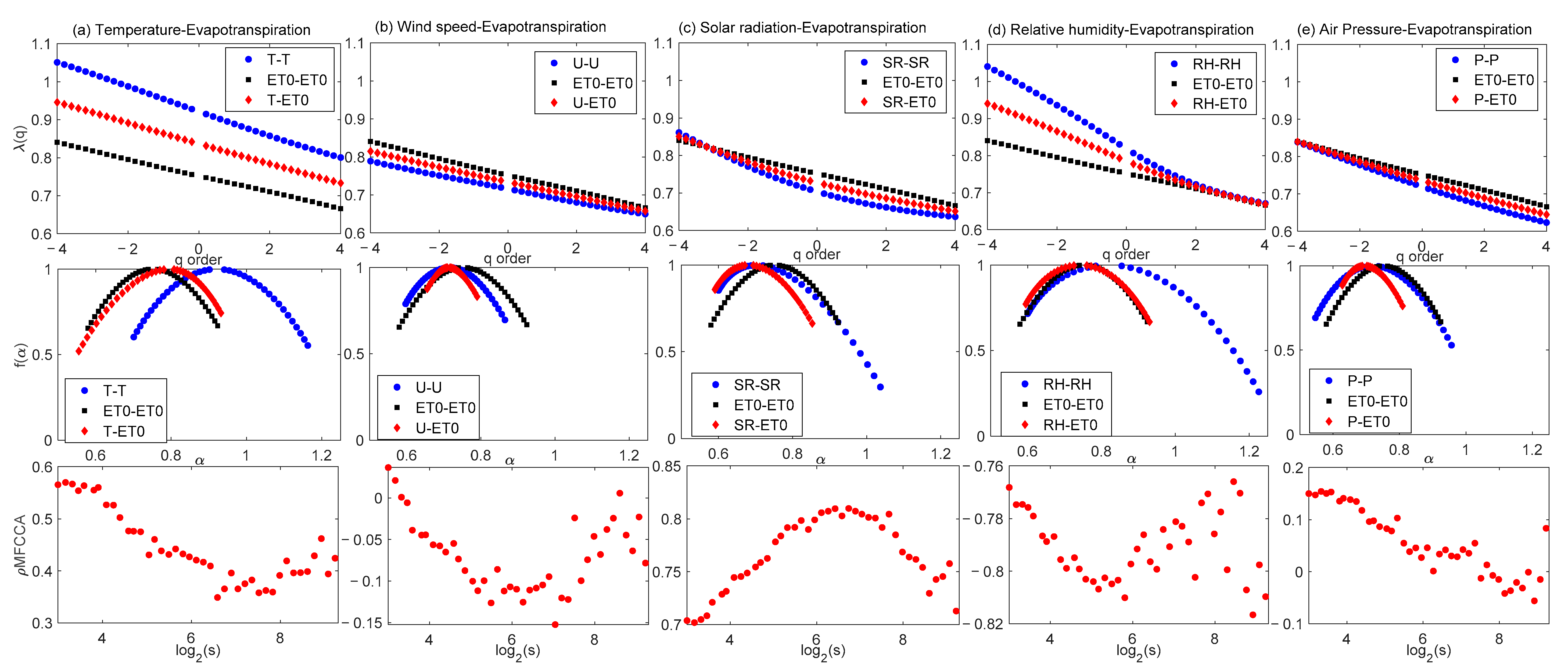
3.2. MFCCA of Meteorological Variables with ET0

Multifractal cross correlation analysis was used to investigate the multiscale cross correlation of different meteorological variables. The scaling exponents were computed for individual time series (with themselves) and the joint scaling exponents were determined for each pair-wise combination with ET0. It is to be noted that in this study results of MFCCA are retrieved for the moment order q = 2 for interpretations and the cross-correlations were determined for different time scales to investigate the change in magnitude and sign [65,66]. Here also a polynomial order m = 1 and a scaling range of [8:600] are chosen for the analysis. Different analysis are performed for q = −4 to 4 to avoid possible elevation bias in the results [60,61]. As the seasonal (90 days) and annual (365 days) time scales are more important for practical applications, these two correlations (seasonal ρ_XY(90) and annual ρ_XY(365)) are calculated separately to investigate the change in magnitude and sign along with the overall Pearson correlation (ρ_o). The graphical representations such as GHE plot, multifractal spectra and cross correlation plots for each link of different stations were prepared. We presented the plots for Dagget and San Diego (highest and lowest altitude stations) as representatives in the Figure 7 and Figure 8, whereas MFCCA plots for other stations are presented in the Supplementary Materials, Figures S9–S11. Detailed examination of different graphical representations of multifractal exponents is made to get an insight into the spatial diversity associations of different variables with ET0 in a multifractal perspective.

The different GHE plots show that the multifractal exponents of air temperature are higher and that of air pressure are lower than the exponents of ET0 irrespective of the station location. Also, the exponents of RH and SR maintain a consistent pattern with respect to the exponents of ET0, for most of the moment orders. In the case of RH time series, the multifractal exponents are less than that of ET0 for all the moment orders more than unity for the three low altitude stations. The multifracral exponents of wind speed are quite similar to that of ET0 for the dataset of LA station, whereas the exponents of U are consistently lower than that of ET0 for the datasets of remaining stations. The similarity in the multifractal exponents of individual time series is reflected in the multifractal spectra also, i.e., if the GHE values, are closer the spectra will be closer and gets dispersed if the GHE plots are distinctly different. But as a universal property, it is noted that the joint multifractal spectra comprise least α values in comparison with the α values of individual spectra. The pattern of correlation plots is strikingly similar in the SR-ET0 link irrespective of the latitude, altitude and location of the station for a time scale up to ~4 months.

In general, it can be noted that the pattern of correlations in different linkages maintain a stable pattern up to 4 months approximately and beyond annul scales, more irregularities are introduced in the correlation behavior in the associations. The pattern of T-ET0 link is similar for the high altitude stations, while a different pattern is noticed for low altitude stations. The correlation behavior mains a definite and consistent pattern in the RH-ET0 link and SR-ET0 link at all the stations, at least up to intra-seasonal scales. The behavior of U-ET0 link is also found to be similar at all the stations except SM, where the association cannot be generalized because of highly complex behavior of the wind speed time series (Figure S10 in the Supplementary Materials).

Additionally, it was observed that air temperature and solar radiation are positively cross-correlated with ET0, regardless of time scale and location, whereas relative humidity is negatively (anti) cross-correlated with ET0. For air pressure situation is more complicated, as the character of cross correlation with ET0 depends both on time scale and location. For the stations with the highest altitudes (Dagget and Bakersfield) P-ET0 is negatively cross-correlated at most of the time scales, while for stations closer to the coastline the sign of cross-correlation changes from positive to negative at larger time scales beyond the intra-seasonal range. There exists a weak positive power law correlation in the U-ET0 links of all the stations, except the two altitude stations of Los Angeles and San Diego. In the U-ET0 linkages of these two stations, a transition in cross-correlation behavior from positive to negative at larger time scales is noticed.

A more important point is that MFCCA could successfully capture such transitions in the nature of power law cross correlation in different agro-meteorological linkages. Such scale specific transitions in the nature of associations could also be explored using other potential methods like wavelet coherence or Time Dependent Intrinsic Correlation [87,88]. One cannot ignore the influence of local climatological drivers and interplay between different meteorological variables resulted in such dynamics in the nature of association of different variables with ET0. The annual and seasonal power law correlations along with the overall correlations in different linkages are presented in

Table 3. MFCCA parameters of different agro-meteorological datasets of California, supplemented with Pearson correlation coefficient (ρ_o).

Link	MFCCA Parameters											Pearson Correlation Coefficient
	Scaling Exponent			Spectral Width			Asymmetry Index			Cross Correlation Coefficient
	λXX	λYY	λXY	WXX	WYY	WXY	AIXX	AIYY	AIXY	ρXY(90)	ρXY(365)	ρ
Dagget
T-ET0	0.896	0.778	0.837	0.300	0.426	0.218	−0.522	−0.325	−0.473	0.575	0.610	0.560
U-ET0	0.619	0.778	0.699	0.417	0.426	0.276	−0.452	−0.325	−0.454	0.256	0.416	0.465
SR-ET0	0.708	0.778	0.743	0.548	0.426	0.365	−0.348	−0.325	0.071	0.615	0.610	0.447
RH-ET0	0.868	0.778	0.823	0.482	0.426	0.273	−0.341	−0.325	−0.018	−0.652	−0.633	−0.508
P-ET0	0.619	0.778	0.699	0.413	0.426	0.139	−0.369	−0.325	−0.237	0.033	0.019	−0.169
Bakersfield
T-ET0	0.824	0.804	0.814	0.374	0.440	0.276	−0.379	−0.468	−0.138	0.707	0.585	0.617
U-ET0	0.690	0.805	0.748	0.369	0.515	0.351	−0.786	−0.468	0.068	0.136	0.310	0.402
SR-ET0	0.719	0.804	0.762	0.491	0.440	0.317	−0.396	−0.468	−0.019	0.668	0.684	0.571
RH-ET0	0.855	0.804	0.830	0.309	0.440	0.210	−0.445	−0.468	−0.287	−0.784	−0.706	−0.700
P-ET0	0.675	0.804	0.739	0.345	0.440	0.075	−0.220	−0.468	−0.745	−0.145	−0.113	−0.118
Santa Maria
T-ET0	0.881	0.748	0.815	0.351	0.281	0.249	−0.392	−0.463	−0.193	0.462	0.452	0.505
U-ET0	0.630	0.715	0.672	0.483	0.375	0.288	−0.450	−0.220	−0.325	0.084	0.163	0.159
SR-ET0	0.672	0.748	0.710	0.469	0.281	0.272	−0.432	−0.463	−0.354	0.742	0.627	0.679
RH-ET0	0.739	0.748	0.743	0.503	0.281	0.282	−0.381	−0.463	−0.432	−0.811	−0.822	−0.791
P-ET0	0.679	0.748	0.713	0.405	0.281	0.154	−0.180	−0.463	−0.315	0.087	0.088	0.081
Los Angeles
T-ET0	0.853	0.708	0.781	0.514	0.425	0.400	−0.116	−0.177	0.102	0.428	0.454	0.522
U-ET0	0.708	0.708	0.708	0.326	0.425	0.193	−0.158	−0.177	−0.219	0.057	−0.011	0.172
SR-ET0	0.676	0.708	0.692	0.400	0.425	0.266	−0.566	−0.177	−0.328	0.764	0.716	0.681
RH-ET0	0.712	0.708	0.710	0.604	0.425	0.456	−0.286	−0.177	−0.358	−0.863	−0.853	−0.848
P-ET0	0.659	0.708	0.684	0.407	0.425	0.255	−0.176	−0.177	−0.233	0.031	−0.003	0.060
San Diego
T-ET0	0.857	0.711	0.784	0.462	0.344	0.377	−0.049	0.003	0.289	0.385	0.397	0.460
U-ET0	0.681	0.711	0.696	0.268	0.344	0.135	−0.121	0.003	−0.147	−0.110	−0.013	−0.009
SR-ET0	0.662	0.711	0.686	0.437	0.344	0.263	−0.564	0.003	−0.326	0.807	0.745	0.738
RH-ET0	0.722	0.711	0.717	0.626	0.344	0.335	−0.337	0.003	−0.132	−0.798	−0.768	−0.768
P-ET0	0.668	0.711	0.689	0.410	0.344	0.181	−0.168	0.003	−0.285	0.037	−0.025	0.103

λ, W, AI, ρ are dimensionless. Indices XX denote the MFCCA properties of the candidate meteorological variable, YY denote properties of ET0, whereas XY denote the properties of joint series.

. The overall correlations are consistently positive in the T-ET0 and SR-ET0 links, while it is strongly negative in RH-ET0 link, irrespective of the location of the station. There exists a moderate positive correlation in the SR-ET0 link at all stations (0.48–0.74 at different locations), while in the U-ET0 link such correlation is noted only at the two high altitude stations of Dagget and Bakersfield. In the P-ET0 and U-ET0 the overall correlation is very weak, which could also be attributed to the alterations in the nature of correlations with the time scale. i.e., in positive correlations in some of the time scales may get nullified by the negative correlation in some other scale and vice versa. Table 3 shows that strength of the association also could also be time scale dependent. In majority of the linkages, the annual correlations are greater than seasonal correlations. But it is to be noted that, against the general notion of strong associations at annual time scale, a stronger correlations can also be deciphered at seasonal time scales in some cases (see, in the linkages of T and SR with ET0 of stations of Bakersfield and Santa Maria stations). The spectral properties such as asymmetry and spectral width are also calculated for each pair wise analysis of different stations, and all the results are summarized in Table 3. From Table 3, it is noticed that the joint scaling exponent is nearly half of the scaling exponent of the individual series. This is universal property in multifractal cross correlation studies [89], which is found to be valid in different pairs of linkages in different stations of California. Apart from this, the joint multifractal spectral width is found to be lower that of the width of individual spectra in all cases. This can be considered as another universal property in multifractal cross correlation studies. Also, it is noted that despite the similar character (positive or negative) of AI of individual spectra, the joint spectra may be of opposing character. This preliminary study is performed to investigate the differences in the multifractal properties and multifractal correlations considering stations primarily based on altitude of the stations. The location of the different stations shows that the three low altitude stations are located at the coastal belts of California. The oceanic proximity plays a dominant role in the climatology of the country in general, and the stations in particular. The large scale atmospheric circulations from oceans line El Nino and La Nina play a major role on the climatology in the stations like San Diego in particular. Hence the role of these circulations on the multifractal properties of the time series also cannot be ignored. Apart from the global parameters like terrestrial radiations and temperature, the local factors like the latitude, topography and local processes, moisture, vegetation etc. along with oceanic and atmospheric circulations may influence the multifractality of the rainfall series. However it will be hard to find a universal pattern such as how the exponents change with latitude, altitude or distance from the coast and attributing the physical reason for multifractality to single indicator may not be justifiable.

The multiscale power law correlations using MFCCA is first of this kind in agro-meteorological studies. The analysis shows that MFCCA is a robust alternative to investigate the pair wise associations of agro-meteorological datasets in different time scale. The study could successfully capture the dynamics (i.e., the transitions from positive to negative or vice versa) of associations over the time scale. Even though a preliminary investigation is made on differences in the multifractal properties based on altitude and location of the stations, an in-depth investigation on local meteorological processes will be complementary to this understanding in physical context. Also the uncertainty analysis in the quantification of scaling exponents is yet another open research problem in the domain. Moreover, stemming from this pre-requite analysis and parameters derived from it, the multifractal modeling of different variables need to be performed and its potential applicability against the classical time series or and data driven approaches are to be analyzed.

4. Conclusions

This study investigated the multifractality of six agro-meteorological variables from California, USA using MFDFA. The analysis showed that all agro-meteorological time series possess strong long term persistence and multifractality. The persistence of T, ET0 and SR are high at all stations, indicating better predictability of these variables. The Hurst exponent (H) of air pressure and wind speed are moderate (varying between 0.61 and 0.75), irrespective of the location or altitude, whereas the H-value of SR and ET0 increases with increase in altitude of the station. MFCCA is found to be a robust method for investigating the power law correlations in agro-meteorological datasets. MFCCA analysis showed that for all the time series considered, the joint scaling exponent is roughly the average of individual scaling exponents, validating the universal property of multifractal cross correlation studies for agro-meteorological datasets. The multifractal exponents of air pressure and wind speed consistently lower than the exponents of ET0, irrespective of station location. The α-values of joint multifractal spectrum are lower than the α values of both of the individual spectra, indicating a universality in the multifractal cross correlation studies. Additionally, MFCCA method allows assessing the impact of time scale on cross-correlation strength. It successfully captured the dynamics in the nature of associations of P and U time series with ET0 over the time scale. The pattern of correlation plots is strikingly similar in the SR-ET0 link irrespective of the latitude, altitude and location of the station. It was found that in general, the temporal evolution of cross-correlation display diversity in different pair-wise associations involving ET0 for low altitude stations and high altitude stations. Multifractal modeling of agro-meteorological datasets, uncertainty analysis of derived multifractal parameters and in-depth investigation on local meteorological processes in conjunction with the MFCCA are some possible avenues for future research.

References

1. Krzyszczak, J.; Baranowski, P.; Zubik, M.; Hoffmann, H. Temporal scale influence on multifractal properties of agro-meteorological time series. Agric. For. Meteorol. 2017, 239, 223–235. [Google Scholar] [CrossRef]
2. Verrier, S.; de Montera, L.; Barthès, L.; Mallet, C. Multifractal analysis of African monsoon rain fields, taking into account the zero rain-rate problem. J. Hydrol. 2010, 389, 111–120. [Google Scholar] [CrossRef]
3. Shang, P.; Kame, S. Fractal nature of time series in the sediment transport phenomenon. Chaos Solitons Fractals 2005, 26, 997–1007. [Google Scholar] [CrossRef]
4. Mandelbrot, B. The Fractal Geometry of Nature; WH Freeman Publishers: New York, NY, USA, 1982. [Google Scholar]
5. Kolmogorov, A.N. Local structure of turbulence in an incompressible liquid for very large Reynolds numbers. Proc. Acad. Sci. URSS. Geochem. Sect. 1941, 30, 299–303. [Google Scholar]
6. Obukhov, A.M. Spectral Energy Distribution in a Turbulent Flow. Izv. Akad. Nauk. S.S.S.R. Ser. Geogr. Geophys. 1941, 5, 453–466. [Google Scholar]
7. Obukhov, A.M. Structure of the temperature field in a turbulent flow. Izv. Akad. Nauk. S.S.S.R Ser. Geogr. Geofiz. 1949, 13, 58–69. [Google Scholar]
8. Corrsin, S. On the Spectrum of Isotropic Temperature Fluctuations in an Isotropic Turbulence. J. Appl. Phys. 1951, 22, 469–473. [Google Scholar] [CrossRef]
9. Kolmogorov, A.N. A refinement of previous hypotheses concerning the local structure of turbulence in a viscous incompressible fluid at high Reynolds number. J. Fluid Mech. 1962, 13, 82–85. [Google Scholar] [CrossRef] [Green Version]
10. Obukhov, A.M. Some specific features of atmospheric turbulence. J. Fluid Mech. 1962, 13, 77–81. [Google Scholar] [CrossRef]
11. Novikov, E.A.; Stewart, R. Intermittency of turbulence and spectrum of fluctuations in energy-disspation. Izv. Akad. Nauk. SSSR. Ser. Geofiz. 1964, 3, 408–412. [Google Scholar]
12. Yaglom, A.M. The influence of the fluctuation in energy dissipation on the shape of turbulent characteristics in the inertial interval. Sov. Phys. Dokl. 1966, 2, 26–30. [Google Scholar]
13. Mandelbrot, B. Intermittent turbulence in self-similar cascades: Divergence of high moments and dimension of the carrier. J. Fluid Mech. 1974, 62, 331–350. [Google Scholar] [CrossRef]
14. Frisch, U. Turbulence: The Legacy of A.N. Kolmogorov; Cambridge University Press: Cambridge, UK, 1995. [Google Scholar]
15. Seuront, L.; Schmitt, F.; Sherzter, D.; Lagadeue, Y.; Lovejoy, S. Multifractal intermittency of Eulerian and Lagrangian turbulence of ocean temperature and plankton fields. Nonlinear Process. Geophys. 1996, 3, 236–246. [Google Scholar] [CrossRef] [Green Version]
16. Schmitt, F.G.; Huang, Y.-X. Stochastic Analysis of Scaling Time Series; Cambridge University Press: Cambridge, UK, 2016. [Google Scholar]
17. Hurst, H.E. The long-term Storage capacity of Reservoir. Trans. Am. Soc. Civil Eng. 1951, 116, 770–779. [Google Scholar]
18. Tessier, Y.; Lovejoy, S.; Hubert, P.; Schertzer, D.; Pecknold, S. Multifractal analysis and modeling of rainfall and river flows and scaling, causal transfer functions. J. Geophys. Res. 1996, 101, 26427–26440. [Google Scholar] [CrossRef]
19. Schaefer, A.; Brach, J.S.; Perera, S.; Sejdić, E.A. Comparative analysis of spectral exponent estimation techniques for 1/fβ processes with applications to the analysis of stride interval time series. Neurosci. Methods 2014, 222, 118–130. [Google Scholar] [CrossRef] [Green Version]
20. Szolgayova, E.; Laaha, G.; Blöschl, G.; Bucher, C. Factors influencing long range dependence in streamflow of European rivers. Hydrol. Process. 2014, 28, 1573–1586. [Google Scholar] [CrossRef]
21. Schertzer, D.; Lovejoy, S. Physical modelling and analysis of rain and clouds by aniso–tropic scaling multiplicative processes. J. Geophys. Res. 1987, 92, 9693–9714. [Google Scholar] [CrossRef]
22. Muzy, J.-F.; Bacry, E.; Arneodo, A. Multifractal formalism for fractal signals: The structure-function approach versus the wavelet-transform modulus-maxima method. Phys. Rev. E 1993, 47, 875–884. [Google Scholar] [CrossRef] [Green Version]
23. Peng, C.K.; Buldyrev, S.V.; Havlin, S.; Simons, M.; Stanley, H.E.; Goldberger, A.L. Mosaic organization of DNA nucleotides. Phys. Rev. E 1994, 49, 1685. [Google Scholar] [CrossRef] [Green Version]
24. Kantelhardt, J.W.; Zschiegner, S.A.; Koscielny-Bunde, E.; Havlin, S.; Bunde, A.; Stanley, H.E. Multifractal detrended fluctuation analysis of non-stationary time series. Phys. A 2002, 316, 87–114. [Google Scholar] [CrossRef] [Green Version]
25. Dahlstedt, K.; Jensen, H. Fluctuation spectrum and size scaling of river flow and level. Phys. A 2005, 348, 596–610. [Google Scholar] [CrossRef] [Green Version]
26. Huang, Y.-X. Arbitrary Order Hilbert Spectral Analysis Definition and Application to Fully Developed Turbulence and Environmental Time-series. Ph.D. Thesis, University of Lille France, Lille, France, 2009. [Google Scholar]
27. Kantelhardt, J.W.; Koscielny-Bunde, E.; Rybski, D.; Braun, P.; Bunde, A.; Havlin, S. Long-term persistence and multifractality of precipitation and river runoff records. J. Geophys. Res. Atmos. 2006, 111, D1. [Google Scholar] [CrossRef]
28. Zhang, Q.; Xu, C.-Y.; Yu, Z.; Liu, C.-L.; Chen, Y.-D. Multifractal analysis of streamflow records of the East river basin (Pearl river), China. Phys. A 2009, 388, 927–934. [Google Scholar] [CrossRef]
29. Li, E.; Mu, X.; Zhao, G.; Gao, P. Multifractal detrended fluctuation analysis of streamflow in the Yellow River Basin, China. Water 2015, 7, 1670–1686. [Google Scholar] [CrossRef] [Green Version]
30. Tan, X.; Gan, T.W. Multifractality of Canadian precipitation and streamflow. Int. J. Climatol. 2017, 37, 1221–1236. [Google Scholar] [CrossRef]
31. Lin, G.; Chen, X.; Fu, Z. Temporal–spatial diversities of long-range correlation for relative humidity over China. Phys. A 2007, 383, 585–594. [Google Scholar] [CrossRef]
32. Lin, G.; Fu, Z. A universal model to characterize different multi-fractal behaviors of daily temperature records over China. Phys. A 2008, 387, 573–579. [Google Scholar] [CrossRef]
33. Yu, Z.G.; Leung, Y.; Chen, Y.D.; Zhang, Q.; Anh, V.; Zhou, Y. Multifractal analyses of daily rainfall time series in Pearl River basin of China. Phys. A 2014, 405, 193–202. [Google Scholar] [CrossRef] [Green Version]
34. Burgueño, A.; Lana, X.; Serra, C.; Martínez, M.D. Daily extreme temperature multifractals in Catalonia (NE Spain). Phys. Lett. A 2014, 378, 874–885. [Google Scholar] [CrossRef]
35. Ariza-Villaverde, A.B.; Pavón-Domínguez, P.; Carmona-Cabezas, R.; Gutierrez de Rave, E.; Jimenez-Honero, F.J. Joint multifractal analysis of air temperature, relative humidity and reference evapotranspiration in the middle zone of the Guadalquivir river valley. Agric. For. Meteorol. 2019, 278, 107657. [Google Scholar] [CrossRef]
36. Baranowski, P.; Krzyszczak, J.; Slawinski, C.; Hoffmann, H.; Kozyra, J.; Nieróbca, A.; Siwek, K.; Gluza, A. Multifractal analysis of meteorological time-series to assess climate impacts. Clim. Res. 2015, 65, 39–52. [Google Scholar] [CrossRef] [Green Version]
37. Kalamaras, N.; Philippopoulos, K.; Deligiorgi, D.; Tzanis, C.G.; Karvounis, G. Multifractal scaling properties of daily air temperature time series. Chaos Solitons Fractals 2017, 98, 38–43. [Google Scholar] [CrossRef]
38. Madanchi, A.; Absalan, M.; Lohmann, G.; Anvari, M.; Tabar, M.R.R. Strong short-term non-linearity of solar irradiance fluctuations. Sol. Energy 2017, 144, 1–9. [Google Scholar] [CrossRef]
39. Hou, W.; Feng, G.; Yan, P.; Li, S. Multifractal analysis of the drought area in seven large regions of China from 1961 to 2012. Meteorol. Atmos. Phys. 2018, 130, 459–471. [Google Scholar] [CrossRef] [Green Version]
40. Adarsh, S.; Kumar, D.N.; Deepthi, B.; Gayathri, G.; Aswathy, S.S.; Bhagyasree, S. Multifractal characterization of meteorological drought in India using detrended fluctuation analysis. Int. J. Climatol. 2019, 39, 4234–4255. [Google Scholar] [CrossRef]
41. Krzyszczak, J.; Baranowski, P.; Zubik, M.; Kazandjiev, V.; Georgieva, V.; Sławiński, C.; Siwek, K.; Kozyra, J.; Nieróbca, A. Multifractal characterization and comparison of meteorological time series from two climatic zones. Theor. Appl. Climatol. 2019, 137, 1811–1824. [Google Scholar] [CrossRef] [Green Version]
42. Krzyszczak, J.; Baranowski, P.; Hoffmann, H.; Zubik, M.; Sławiński, C. Advances in time series Analysis and Forecasting. In Analysis of Climate Dynamics Across a European Transect Using a Multifractal Method; Rojas, I., Pomares, H., Valenzuela, O., Eds.; Springer International Publishing AG: Cham, Switzerland, 2017; pp. 1–14. [Google Scholar]
43. Adarsh, S.; Nourani, V.; Archana, D.S.; Dharan, D.S. Multifractal description of rainfall fields over India. J. Hydrol. 2020, 586, 124913. [Google Scholar] [CrossRef]
44. Doorenbos, J.; Pruitt, W.O. Crop water requirements. FAO Irrig. Drain. Pap. 1977, 24, 1–179. [Google Scholar]
45. Allen, R.G.; Pereira, L.S.; Raes, D.; Smith, M. Crop evapotranspiration. Guidelines for computing crop water requirements. FAO Irrig. Drain. Pap. 1998, 56, D05109. [Google Scholar]
46. Tabari, H.; Grismer, M.E.; Trajkovic, S. Comparative analysis of 31 reference evapotranspiration methods under humid conditions. Irrig. Sci. 2013, 31, 107–117. [Google Scholar] [CrossRef]
47. Kisi, O.; Çimen, M. Evapotranspiration modeling using support vector machines. Hydrol. Sci. J. 2009, 54, 918–928. [Google Scholar] [CrossRef]
48. Cobaner, M. Reference evapotranspiration based on Class A pan evaporation via wavelet regression technique. Irrig. Sci. 2013, 31, 119–134. [Google Scholar] [CrossRef]
49. Valipour, M.; Sefidkouhi, M.A.G.; Raeini-Sarjaz, M.; Guzman, S.M. A Hybrid Data-Driven Machine Learning Techniquefor Evapotranspiration Modeling in Various Climates. Atmosphere 2019, 10, 311. [Google Scholar] [CrossRef] [Green Version]
50. Adarsh, S.; Sulaiman, S.; Murshida, K.K.; Nooramol, P. Scale-dependent prediction of reference evapotranspiration based on Multivariate Empirical Mode Decomposition. Ain Shams Eng. J. 2018, 9, 1839–1848. [Google Scholar] [CrossRef]
51. Nourani, V.; Elkiran, G.; Abdullah, J. Multi-station artificial intelligence based ensemble modeling of reference evapotranspiration using pan evaporation measurements. J. Hydrol. 2019, 577, 123958. [Google Scholar] [CrossRef]
52. Wilks, D.S. Statistical Methods in Atmospheric Sciences, 2nd ed.; Academic Press: San Diego, CA, USA, 2006. [Google Scholar]
53. Bassingthwaighte, J.B.; Beyer, R.P. Fractal correlation in heterogeneous systems. Phys. D 1991, 53, 71–84. [Google Scholar] [CrossRef]
54. Adarsh, S.; Reddy, M.J. Multi-Scale Spectral Analysis in Hydrology: From Theory to Practice; Taylor & Francis Ltd.: Abingdon, UK; CRC Press: Boca Raton, FL, USA, 2021; p. 400852. [Google Scholar]
55. Piao, L.; Fu, Z. Quantifying distinct associations on different temporal scales: Comparison of DCCA and Pearson methods. Sci. Rep. 2016, 6, 36759. [Google Scholar] [CrossRef] [Green Version]
56. Podobnik, B.; Stanley, H.E. Detrended cross-correlation analysis: A new method for analyzing two non-stationary time series. Phys. Rev. Lett. 2008, 100, 084102. [Google Scholar] [CrossRef] [Green Version]
57. Zhou, W.X. Multifractal detrended cross-correlation analysis for two non-stationary signals. Phys. Rev. E 2008, 77, 066211. [Google Scholar] [CrossRef] [Green Version]
58. Jiang, Z.Q.; Zhou, W.X. Multifractal detrending moving-average cross-correlation analysis. Phys. Rev. E 2011, 84, 016106. [Google Scholar] [CrossRef] [PubMed] [Green Version]
59. Oświȩcimka, P.; Drożdż, S.; Forczek, M.; Jadach, S.; Kwapień, J. Detrended cross-correlation analysis consistently extended to multifractality. Phys. Rev. E 2014, 89, 023305. [Google Scholar] [CrossRef] [PubMed] [Green Version]
60. Wątorek, M.; Drożdż, S.; Oświęcimka, P.; Stanuszek, M. Multifractal cross-correlations between the world oil and other financial markets in 2012–2017. Energy Econ. 2019, 81, 874–885. [Google Scholar] [CrossRef] [Green Version]
61. Drożdż, S.; Minati, L.; Oświȩcimka, P.; Stanuszek, M.; Wątorek, M. Signatures of the Crypto-Currency Market Decoupling from the Forex. Future Internet 2019, 11, 154. [Google Scholar] [CrossRef] [Green Version]
62. Zhang, C.; Ni, Z.; Ni, L. Multifractal detrended cross-correlation analysis between PM2.5 and meteorological factors. Phys. A 2015, 438, 114–123. [Google Scholar] [CrossRef]
63. Kar, A.; Chatterjee, S.; Ghosh, D. Multifractal detrended cross-correlation analysis of Land-surface temperature anomalies and Soil radon concentration. Phys. A 2019, 521, 236–247. [Google Scholar] [CrossRef]
64. Tzanis, C.G.; Koutsogiannis, I.; Philippopoulos, K.; Kalamaras, N. Multifractal Detrended Cross-Correlation Analysis of Global Methane and Temperature. Remote Sens. 2020, 12, 557. [Google Scholar] [CrossRef] [Green Version]
65. Zebende, G.F. DCCA cross-correlation coefficient: Quantifying level of cross-correlation. Phys. A 2011, 390, 614–618. [Google Scholar] [CrossRef]
66. Vassoler, R.T.; Zebende, G.F. DCCA cross-correlation coefficient apply in time series of air temperature and air relative humidity. Phys. A 2012, 391, 2438–2443. [Google Scholar] [CrossRef] [Green Version]
67. Wu, Y.; He, Y.; Wu, M.; Lu, C.; Gao, S.; Xu, Y. Multifractality and cross correlation analysis of streamflow and sediment fluctuation at the apex of the Pearl River Delta. Sci. Rep. 2018, 8, 16553. [Google Scholar] [CrossRef]
68. Dey, P.; Mujumdar, P.P. Multiscale evolution of persistence of rainfall and streamflow. Adv. Water Resour. 2018, 121, 285–303. [Google Scholar] [CrossRef]
69. Adarsh, S.; Dharan, D.S.; Nandhu, A.R.; Vishnu, B.A.; Mohan, V.K.; Watorek, M. Multifractal description of streamflow and suspended sediment concentration data from Indian river basins. Acta Geophys. 2020, 68, 519–535. [Google Scholar] [CrossRef] [Green Version]
70. Cleveland, R.B.; Cleveland, W.S.; McRae, J.; Terpenning, I. STL: A seasonal-trend decomposition procedure based on loess. J. Off. Stat. 1990, 6, 3–73. [Google Scholar]
71. López, J.L.; Contreras, J.G. Performance of multifractal detrended fluctuation analysis on short time series. Phys. Rev. E 2013, 87, 022918. [Google Scholar] [CrossRef] [PubMed] [Green Version]
72. Baranowski, P.; Gos, M.; Krzyszczak, J.; Siwek, K.; Kieliszek, A.; Tkaczyk, P. Multifractality of meteorological time series for Poland on the base of MERRA-2 data. Chaos Solitons Fractals 2019, 127, 318–333. [Google Scholar] [CrossRef]
73. Ihlen, E.A.F.E. Introduction to multifractal detrended fluctuation analysis in MATLAB. Front. Physiol. 2012, 3, 141. [Google Scholar] [CrossRef] [Green Version]
74. Yuan, N.; Fu, Z.; Mao, J. Different scaling behaviors in daily temperature records over China. Phys. A 2010, 389, 4087–4095. [Google Scholar] [CrossRef]
75. Köppen, W. VersucheinerKlassifikation der Klimate, vorzugsweise nach ihren Beziehungen zur Pflanzenwelt. Geogr. Z. 1900, 6, 657–679. [Google Scholar]
76. Center for Exposure Assessment Modeling (CEAM), United States Environmental Protection Agency (EPA). Meteorological Data for California. Available online: https://www.epa.gov/ceam/meteorological-data-california (accessed on 18 October 2020).
77. Feng, S.; Hu, Q.; Qian, W. Quality control of daily meteorological data in China, 1951–2000: A new dataset. Int. J. Climatol. 2004, 24, 853–870. [Google Scholar] [CrossRef]
78. Estévez, J.; García-Marín, A.P.; Morábito, J.A.; Cavagnaro, M. Quality assurance procedures for validating meteorological inputvariables of reference evapotranspiration in Mendoza province (Argentina). Agric. Water Manag. 2016, 172, 96–109. [Google Scholar] [CrossRef]
79. Herrera-Grimaldi, P.; Garcia-Marin, A.P.; Estevez, J. Multifractal analysis of diurnal temperature range over Southern Spain using validated datasets. Chaos 2019, 29, 063105. [Google Scholar] [CrossRef] [PubMed]
80. Kisi, O. Daily pan evaporation modelling using a neuro-fuzzy computing technique. J. Hydrol. 2006, 329, 636–646. [Google Scholar] [CrossRef]
81. Makowiec, D.; Fuliński, A. Multifractal Detrended Fluctuation Analysis as the Estimator of Long-range Dependence. Acta Phys. Polonica B 2010, 41, 1025. [Google Scholar]
82. Movahed, M.S.; Jafari, G.R.; Ghasemi, F.; Rahvar, S.; Tabar, M.R.R. Multifractal detrended fluctuation analysis of sunspot time-series. J. Stat. Mech. Theory Exp. 2006, 2006, P02003. [Google Scholar] [CrossRef] [Green Version]
83. Matia, K.; Ashkenazy, Y.; Stanley, H.E. Multifractal properties of price fluctuations of stocks and commodities. Europhys. Lett. 2003, 61, 422–428. [Google Scholar] [CrossRef] [Green Version]
84. Keylock, C.J. A resampling method for generating synthetic hydrological time-series with preservation of cross correlative structure and higher-order properties. Water Resour. Res. 2012, 48, W12521. [Google Scholar] [CrossRef]
85. Schreiber, T.; Schmitz, A. Improved surrogate data for nonlinearity tests. Phys. Rev. Lett. 1996, 77, 635–638. [Google Scholar] [CrossRef] [PubMed] [Green Version]
86. Keylock, C.J. Hypothesis testing for nonlinear phenomena in the geosciences using synthetic, surrogate data. Earth Space Sci. 2019, 6, 41–58. [Google Scholar] [CrossRef]
87. Grinsted, A.; Moore, J.C.; Jevrejeva, S. Application of the cross wavelet transform and wavelet coherence to geophysical time series. Nonlinear Process. Geophys. 2004, 11, 561–566. [Google Scholar] [CrossRef]
88. Huang, Y.-X.; Schmitt, F.G. Time dependent intrinsic correlation analysis of temperature and dissolved oxygen time series using empirical mode decomposition. J. Mar. Syst. 2014, 130, 90–100. [Google Scholar] [CrossRef] [Green Version]
89. Hajian, S.; Movahed, M.S. Multifractal detrended cross-correlation analysis of sunspot numbers and river flow fluctuations. Phys. A 2010, 389, 4942–4954. [Google Scholar] [CrossRef] [Green Version]
Figure 1. Map showing the locations of five meteorological stations in California, USA.
Atmosphere 11 01116 g001
Figure 2. Time series plots of agro-meteorological datasets of different stations in California: (a) Dagget; (b) Bakersfield; (c) Santa Maria; (d) Los Angeles; (e) San Diego.
Atmosphere 11 01116 g002
Figure 3. Fluctuation function plots of different agro-meteorological time series of different stations for q = 2. (a) reference evapotranspiration; (b) temperature; (c) wind speed; (d) solar radiation; (e) relative air humidity; and (f) air pressure.
Atmosphere 11 01116 g003
Figure 4. Multifractal plots of different agro-meteorological time series: (a) reference evapotranspiration; (b) temperature; (c) wind speed; (d) solar radiation; (e) relative air humidity; and (f) air pressure. The upper panels show the GHE plots, middle panels show the mass exponent plots and lower panels show the multifractal spectra.
Atmosphere 11 01116 g004
Figure 5. Fourier spectrum of different agro-meteorological time series of Dagget station. (a) reference evapotranspiration; (b) temperature; (c) wind speed; (d) solar radiation; (e) relative air humidity; and (f) air pressure.
Atmosphere 11 01116 g005
Figure 6. GHE plots of original, shuffled and surrogate series of different agro-meteorological variables of Dagget station: (a) reference evapotranspiration; (b) temperature; (c) wind speed; (d) solar radiation; (e) relative humidity; and (f) air pressure.
Atmosphere 11 01116 g006
Figure 7. GHE plots (upper panels), multifractal spectra (middle panels) and cross-correlation plots (lower panels) obtained by MFCCA of different links at Dagget station: (a) T-ET0; (b) U-ET0; (c) SR-ET0; (d) RH-ET0; (e) P-ET0.
Atmosphere 11 01116 g007
Figure 8. GHE plots (upper panels), multifractal spectra (middle panels) and cross-correlation plots (lower panels) obtained by MFCCA of different links at San Diego station: (a) T-ET0; (b) U-ET0; (c) SR-ET0; (d) RH-ET0; (e) P-ET0.
Atmosphere 11 01116 g008