Article

Trends and Persistence of Dry–Wet Conditions in Northeast Brazil

by
Antonio Samuel Alves da Silva
1,
Moacyr Cunha Filho
1,
Rômulo Simões Cezar Menezes
2,
Tatijana Stosic
1 and
Borko Stosic
1,*
1
Departamento de Estatística e Informática, Universidade Federal Rural de Pernambuco, Rua Dom Manoel de Medeiros s/n, Dois Irmãos, 52171-900 Recife/PE, Brazil
2
Departamento de Energia Nuclear, Universidade Federal de Pernambuco, Moraes Rego 1235, Cidade Universitária, 50670-901 Recife-PE, Brazil
*
Author to whom correspondence should be addressed.
Atmosphere 2020, 11(10), 1134; https://doi.org/10.3390/atmos11101134
Submission received: 9 October 2020 / Accepted: 16 October 2020 / Published: 21 October 2020
(This article belongs to the Special Issue Climate Change and Agrometeorological Time Series)

Abstract

:
We analyze trend and persistence in Standardized Precipitation Index (SPI) time series derived from monthly rainfall data at 133 gauging stations in Pernambuco state, Brazil, using a suite of complementary methods to address the spatially explicit tendencies, and persistence. SPI was calculated for 1-, 3-, 6-, and 12-month time scales from 1950 to 2012. We use Mann–Kendall test and Sen’s slope to determine sign and magnitude of the trend, and detrended fluctuation analysis (DFA) method to quantify long-term correlations. For all time scales significant negative trends are obtained in the Sertão (deep inland) region, while significant positive trends are found in the Agreste (intermediate inland), and Zona da Mata (coastal) regions. The values of DFA exponents show different scaling behavior for different time scales. For short-term conditions described by SPI-1 the DFA exponent is close to 0.5 indicating weak persistency and low predictability, while for medium-term conditions (SPI-3 and SPI-6) DFA exponents are greater than 0.5 and increase with time scale indicating stronger persistency and higher predictability. For SPI-12 that describes long-term precipitation patterns, the values of DFA exponents for inland regions are around 1, indicating strong persistency, while in the shoreline the value of the DFA exponent is between 1.0 and 1.5, indicating anti-persistent fractional Brownian motion. These results should be useful for agricultural planning and water resource management in the region.

1. Introduction

Rainfall variability leads to a deficit or excess of water with respect to normal conditions at a given location. Severity and duration of these anomalies have a direct effect on availability of water resources and can compromise agricultural productivity, food security, water resource management, land use, human health and ecological equilibrium [1,2,3,4]. Extreme rainfall related events as severe floods and drought have been observed in many tropical countries and it is expected to increase in severity during this century [5]. Several indices have been developed to evaluate the severity of dry/wet conditions including the Palmer Drought Severity index (PDSI) [6], the Standardized Runoff Index (SRI) [7], the Standardized Precipitation Index (SPI) [8] and Standardized Precipitation Evapotranspiration Index (SPEI) [9]. Among them, the SPI stands out from the point of view that it only requires rainfall data for computations (and no other additional variables or empirical parametrizations), it can be compared among different regions with different climatic conditions [10], and it has already been widely applied to analyze dry/wet conditions in different parts of the world, in many different contexts [11,12,13,14,15].
Over the last decades Brazil has been affected by several severe drought events: Northeast Brazil (NEB) experienced drought in 2010–2016; Southeastern Brazil in 2014–15, and Amazonia in 2005, 2010 and 2016 [16]. Droughts are widespread and recurrent in the semiarid NEB region, which represents the world’s most densely populous dry land region. With more than 53 million inhabitants, density of ∼34 inhabitants per square kilometer, and a highest proportion of people living in poverty in Brazil, the NEB region is one of the world’s most vulnerable areas to the impacts of climate change [17,18]. Based on several studies [19,20], it is expected that the risk of natural disasters related to excess or lack of water (flash floods and severe droughts) will continue increasing in the region until the end of the century. There are several studies that address drought in NEB [18,21], including some specific regions as states of Rio Grande de Norte [22], Alagoas [23] and Paraiba [24].
This work aims to contribute to a better understanding of the spatio-temporal distribution of dry/wet conditions in Northeast Brazilian, specifically the state of Pernambuco, with a large part (about 70% of total territory) located in the so called “Drought Polygon” (Poligono das Secas), making it extremely vulnerable to seasonal and inter-annual rainfall variability. We analyze trends and persistence of dry/wet categories by applying Mann Kendall test and detrended fluctuation analysis on temporal series of Standardized Precipitation Index, calculated for different time scales (1–12 months). The results for 133 pluviometric stations which, are well (rather uniformly) distributed over all parts of Pernambuco are used to analyze spatial distribution of characteristics of the rainfall regime.

2. Material and Methods

2.1. Study Area and Dataset

Pernambuco is a state in the NEB region, located between the parallels 7 ° 15 45   S and 9 ° 28 18   S and meridians 34 ° 48 33   W and 41 ° 19 54   W , bordering the states of Paraiba and Ceará (north), Piaui (west), Alagoas and Bahia (south), and limited to the east by the Atlantic Ocean. As shown in Figure 1, the state is divided into three geographic regions: the forest zone (Zona da Mata) that comprises a coastal strip from the sea to the mountain chain called Borborema, about 70 km away, transition zone (Agreste), and to the west of Borborema the region known as Sertão, which is far less populated because of the arid climate. Sertão region is mostly covered by Caatinga—a semiarid biome which is dominated by shrub vegetation as well as by tropical dry forests. Coastal region Zona da Mata consists of fragments of the Atlantic rain forest, predominantly located on the tops of low hills (50–100 m high), surrounded by sugar cane fields at lower elevations. Agreste is a transition zone, where Atlantic forest mixes with Caatinga [25,26]. In the coastal area the climate is tropical with a strong rainfall gradient (east to west) from 1500 to 700 mm annual rainfall, with the rainy season concentrated between May and July, and the intense dry season between September and December. Semiarid climate covering 61.4% of the territory occurs along the depressions and plains of Sao Francisco River, and stretches almost everywhere in the hinterland region, where the annual rainfall is less than 500 mm, concentrated from February to April, and a dry period lasts nine months [27].
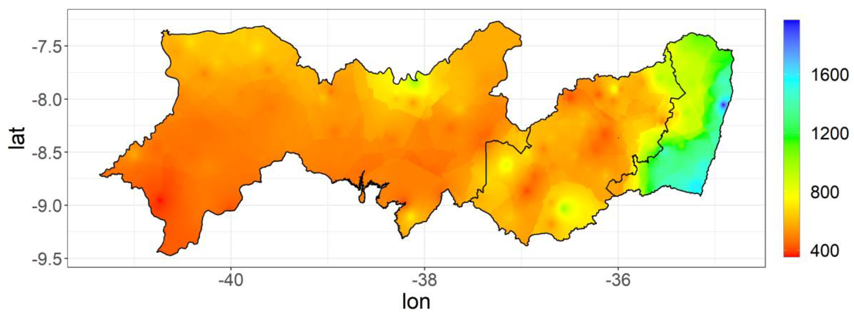
The data used in this work are historical series of monthly precipitation for the state of Pernambuco, Brazil, provided by the Meteorological Laboratory of the Institute of Technology of Pernambuco (Laboratório de Meteorologia do Instituto de Tecnologia de Pernambuco—LAMEP/ITEP). The monthly series of precipitation, with time span from 1950 to 2012, corresponds to records obtained from 133 meteorological stations as shown in Figure 1, together with the digital elevation model (DEM) data. The missing data were filled using the trend surface analysis interpolation method [28]. The study period was selected as a trade-off between the series length and the number of stations, where stations with over 10% of missing data were discarded. The resulting interpolated mean annual precipitation is shown in Figure 2. All the analyses were performed in R [29], with the help of the contributed package trend [30].

2.2. Standardized Precipitation Index

The Standardized Precipitation Index (SPI), developed by McKee et al. [8] to quantify the precipitation deficit for multiple time scales (i.e., 1, 3, 6, 12, 24 and 48 months), is recommended by the World Meteorological Organization (WMO) as an index to characterize drought severity [31]. For calculation of the SPI, first it is necessary to adjust the probability density function (pdf) for the precipitation dataset. Among several distributions proposed in the literature [32,33], in this work we adopt the gamma distribution, which is the most widely used to fit precipitation time series [8,34]. The gamma pdf is given by
f ( x ) =   1 β α Γ ( α ) x α 1 e x / β ,    x > 0
where α > 0 is a shape parameter, β > 0 is a scale parameter, x is the amount of precipitation and Γ ( α ) is gamma function Γ ( α ) = 0 y α 1 e y d y . The parameters α and β are estimated using maximum likelihood method, which yields estimates
α ^ =   1 4 A ( 1 + 1 + 4 A 3 )        ,        β ^ = β ^ x ¯ α ^
where x ¯ is the average value of precipitation quantity, notation A   ln ( x ¯ ) Σ   ln x n is used to provide a more compact formula representation, and n is the number of observations [35]. Next, f ( x ) is integrated with respect to x , to obtain the cumulative probability
F ( x ) =   0 x f ( x ) d x = 1 β ^ α ^ Γ ( α ^ ) 0 x x α ^ 1 e x / β ^ d x .
The gamma function is undefined for x = 0 , and as naturally precipitation data does contain zeros, the cumulative probability is taken to be
H ( x ) = q + ( 1 q ) F ( x )
where q is the probability of zero (null) precipitation, which is calculated as   q = m / n , where m represents the number of zeros in a precipitation series and n is the number of observations. Finally, the SPI is generated by standardizing the values obtained in H ( x ) [36,37]
S P I = { ( t c 0   +   c 1 t   +   c 2 t 2 1   +   d 1 t   +   d 2 t 2   +   d 3 t 3 ) ,    0 < H ( x ) < 0.5   +   ( t c 0   +   c 1 t   +   c 2 t 2 1   +   d 1 t   +   d 2 t 2   +   d 3 t 3 ) ,    0.5 < H ( x ) 1.0
with c 0 =   2.515517; c 1 =   0.802853; c 2 =   0.010328; and d 1 =   1.432788; d 2 =   0.189269; d 3 =   0.001308, and t is given by
t = { ln [ 1 ( H ( x ) ) 2 ] ,    0 < H ( x ) < 0.5 ln [ 1 ( 1 H ( x ) ) 2 ] ,    0.5 < H ( x ) 1.0
McKee et al. [8] categorize the SPI into moderate, severe and extreme classes for both dry and wet conditions as shown in the Table 1.
The 1-month SPI is related to meteorological types of drought together with short-term soil moisture and crop stress, SPI-3 reflects medium-term soil moisture conditions, while 6-month and 12-month SPI indicate seasonal to long-term precipitation temporal patterns and are associated with anomalous streamflows, and reservoir and ground water levels [10].
In this study, the 1- and 3-month SPI are used to represent short-term and seasonal drought, the 6-month SPI is used for intermediate-term drought, and the 12-month SPI is used for long-term drought. In all cases the whole period is used to adjust the gamma pdf.

2.3. Mann–Kendall Test

The Mann–Kendall test [38,39] is a non-parametric statistical method (it does not require that data follow any specific distribution) used to determine whether a time series has a monotonic upward or downward trend. It is a rank-based procedure, especially suitable for non-normally distributed data, data containing outliers, and nonlinear trends [40]. This test is based on the correlation between the values of time series and their temporal order, the null hypothesis being that the observations are independent and identically distributed (no trend), and the alternative hypothesis being that there is a monotonic trend (upward or downward). For the times series x 1 , x 2 , ,   x n the Mann–Kendall test uses the statistic
S = i = 1 n 1 j = i + 1 n s g n ( x j x i )
where x i and x j are the sequential data values, n is the length of the dataset, and s g n ( . )
Stands for the sign of the argument, with
s g n ( x j x i ) = { 1 , x j > x i 0 , x   j = x i 1 , x j < x i
Under the assumption that the data are independent and identically distributed (null hypothesis), the S statistics has mean zero, E ( S ) = 0 , and variance given by
V a r ( S ) = 1 18 [ n ( n 1 ) ( 2 n + 5 ) p = 1 q t p ( t p 1 ) ( 2 t p + 5 ) ]
in which q is   the   number   of   tied   groups , and t p is the number of observations in the p -th group. The test statistic Z , which has a normal distribution, is computed based on the values S and V a r ( S )
Z = { S 1 V a r ( S ) ,            S > 0          0     ,     S = 0 S + 1 V a r ( S ) ,            S < 0
Positive values of Z indicate upward trends, while negative values of Z show downward trends. Finally, for testing purposes the p value ( p v ) is computed as
p v = 2 min ( ϕ ( Z ) , 1 ϕ ( Z ) )
where min ( · , · ) stands for the minimum of the two arguments, and ϕ ( · ) is the cumulative distribution function of the standard normal distribution—the null hypothesis is rejected when the p value of the test standardized statistic Z is less than the chosen significance level α . Therefore, the trend is said to be downward if Z is negative and upward if Z is positive, and the p v is less than α . In this paper, we used the significance level α = 0.05 . The Mann Kendall non-parametric test has been widely used to quantify the trends in hydro-meteorological times series [41,42,43].

2.4. Wilcoxon–Mann–Whitney Test

The Wilcoxon–Mann–Whitney test [44,45], is a non-parametric hypothesis test used to check whether or not two independent samples containing n 1 and n 2 elements correspond to the same distribution. It does not require the data normality assumption. The Wilcoxon–Mann–Whitney statistic W is computed as follows: the n 1   +   n 2 observations of the two independent samples are combined in a single dataset. The elements of this dataset are sorted from smallest to largest. If there are ties in the combined dataset, the ranks for the observations in a tie are taken to be the average of the ranks for those observations. The Wilcoxon statistic, W , is calculated as the sum of ranks of the sample with the smaller sample size. Under this null hypothesis, the expectation and variance of W are, respectively
μ W = n 1 ( n 1 + n 2 + 1 ) 2   and      σ W 2 = n 1 n 2 ( n 1 + n 2 + 1 ) 12 .
For n 1 and n 2 greater than 10, the distribution of the statistic T = ( W μ W ) / σ W can be approximated by a normal distribution with zero expectation and variance equal to unity. In the case of ties the variance needs to be modified for the Gaussian approximation. Let n t be the number of groups with ties and t k the number of ties in group k then
    σ W 2 = n 1 n 2 12 [ n 1 +   n 2 + 1 k = 1 n t ( t k 3 t k ) / ( ( n 1 +   n 2 ) ( n 1 +   n 2 1 ) ) ] .
Under this assumption, the p value ( p v ) is calculated as
p v = 2 [ 1 ϕ ( | w μ W | σ W ) ] ,
where w denotes the value of the rank-sum statistic in the sample, and ϕ ( · ) is the cumulative distribution function of the standard normal distribution. For a specific significance level α ( 0 ,   1 ) , the null hypothesis is rejected whenever p v   <   α .

2.5. Sen’s Slope of Trend

The Mann Kendall test is an efficient method for identifying trends in time series, but it does not provide the magnitude of the trend. It can be complemented by the non-parametric method proposed by Sen [46] to estimate the true slope of an existing trend. The main strength of the Sen slope estimator is its robustness to the presence of outliers [47,48]. The slopes of all data value pairs are calculated as
Q i , j = x j x i j i ,    i = 1 ,   ,   n 1      ;     j = i + 1 , , n
where x i and x j are the data values at times i and j ( i < j ), respectively. If the analyzed series has n values, then the number of pairs Q i , j is N = n ( n 1 ) / 2 . Finally, the slope median Q med (or Sen’s slope estimator) is calculated: the sign of Q med reflects the data (upward or downward) trend, while its value indicates the steepness of the trend.

2.6. Detrended Fluctuation Analysis

Detrended fluctuation analysis (DFA) was introduced by Peng et al. [49] as a method for quantification of correlations in non-stationary time series [50,51]. This method represents a modified root-mean-square analysis of a random walk, and was successfully applied in physiological processes [52], geophysical signals [53], climatic records [54,55], hydrological time series [56] and financial data [57]. The implementation of the DFA algorithm is described as follows:
(i)
The original temporal series x ( i ) , i = 1 , 2 , , N is integrated to calculate
X ( k ) = i = 1 k [ x ( i ) x ] ,   k = 1 , 2 , , N
where x = Σ i = 1 N x ( i ) / N is the average.
(ii)
Next, the integrated series X ( k ) is divided into N n = i n t ( N / n ) non-overlapping segments of length n (here i n t ( · ) stands for the integer value of the argument), and in each segment s = 1 , ,   N n the local trend X n . s ( k ) (linear or higher order polynomial least square fit—termed DFA1, DFA2, DFA3,…, for polynomials of order 1,2, 3,…, respectively) is estimated and subtracted from X ( k ) . In DFAm, trends of order m in the profile X ( k ) , and of order m 1 in the original record x ( i ) are eliminated.
(iii)
The detrended variance is now calculated as
F 2 ( n ) = 1 n N s = 1 N n k = ( s 1 ) n + 1 s n [ X ( k ) X n , s ( k ) ] 2
(iv)
Repeating this calculation for different window sizes provides the relationship between the fluctuation function F ( n ) and the window size n . If long-term correlations are present in original series, F ( n ) increases with n according to a power law
F ( n )   ~   n α
The scaling exponent α is obtained as the slope of the linear regression of log F ( n ) versus log n . The value α = 0.5 indicates the absence of correlations (white noise), α > 0.5 indicates persistence of long-term correlations, meaning that large (small) values are more likely to be followed by large (small) values, while α < 0.5   indicates anti-persistent long-term correlations, meaning that large values are more likely to be followed by small values, and vice versa. The values α = 1 and α = 1.5 correspond to 1 / f noise and Brownian noise (integration of white noise), respectively [49].

3. Results and Discussion

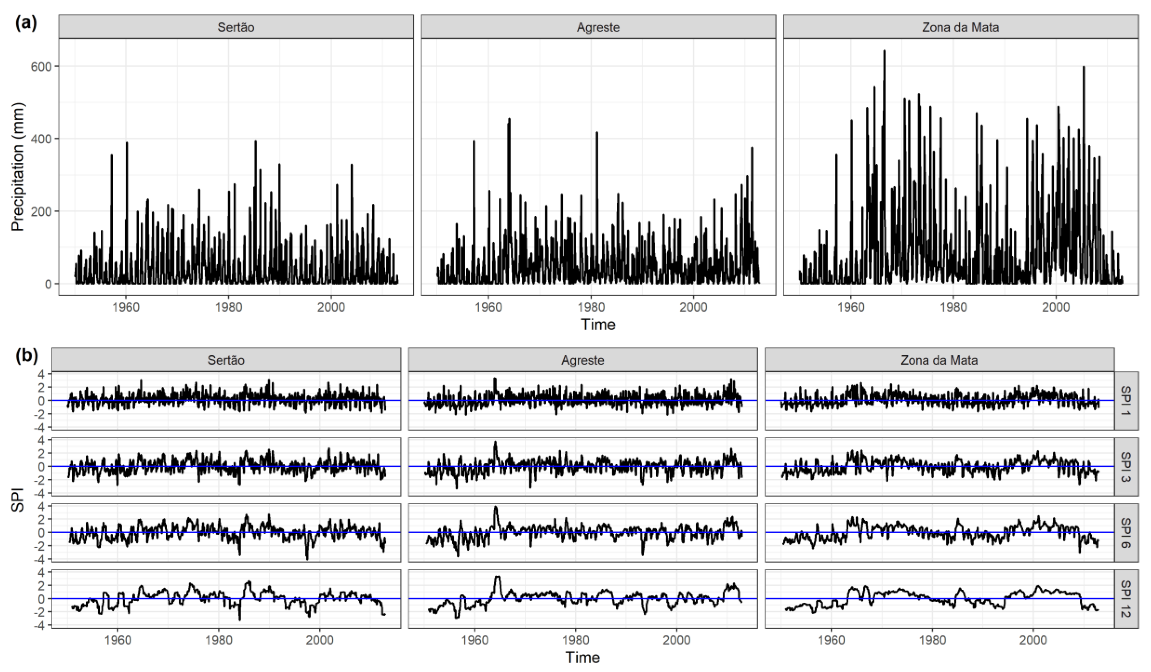
Monthly precipitation data for representative stations of the three regions, together with the calculated SPI values on time scales 1, 3, 6 and 12 months are shown in Figure 3.

3.1. Trend Analysis

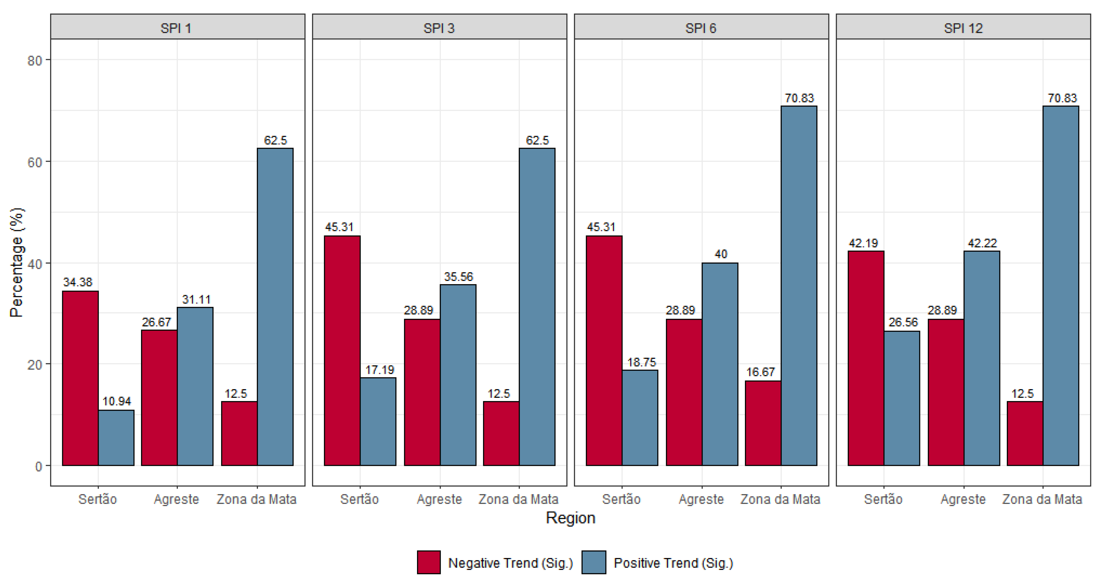
The results of the trend analysis for the series of SPI values (time scale 1, 3, 6 and 12 months) for regions Sertão, Agreste and Zona da Mata are summarized in Figure 4. This figure shows the percentage of stations with significant trends ( p v < 0.05 ) for each of the SPI time scales and for each region. Higher percentages of significant negative trend are obtained in the Sertão region, for all time scales. On the other hand, higher percentages of significant positive trends are found in Agreste and Zona da Mata, with the percentage obtained in Zona da Mata region (close to the coast) always higher than that obtained in the (inland) Agreste region.
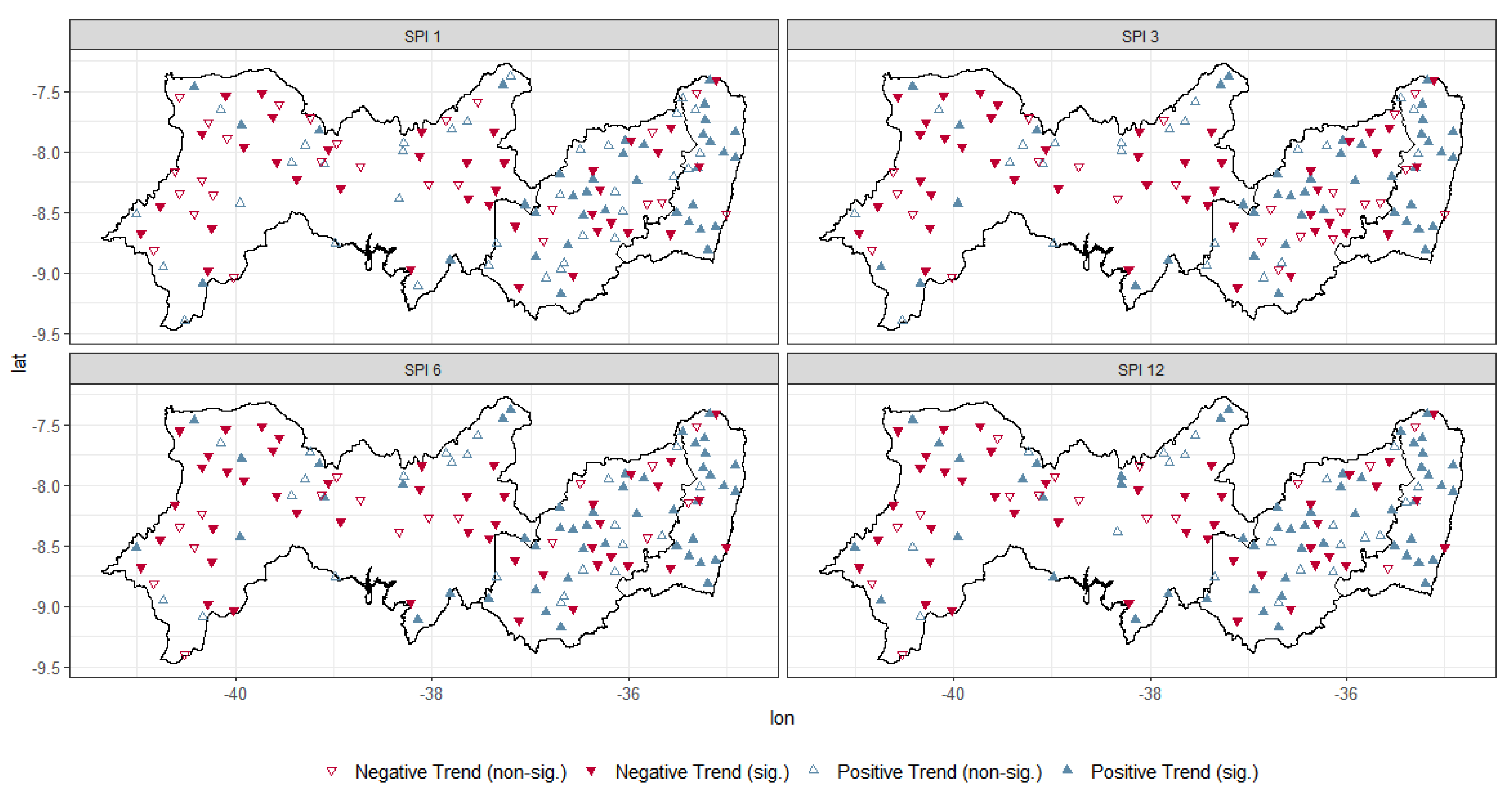
For all time scales, percentage of non-significant trends ( p v 0.05 ) is lower than the percentage of significant trends. These percentages are 45% (26% Sertão, 14% Agreste, 5% Zona da Mata), 35% (18% Sertão, 12% Agreste, 5% Zona da Mata), 30% (17% Sertão, 11% Agreste, 2% Zona da Mata) and 28% (15% Sertão, 10% Agreste, 3% Zona da Mata) for time scales 1, 3, 6 and 12, respectively. Spatial distributions of trends (significant and non-significant) for the series of SPI values for time scales 1, 3, 6 and 12 months are shown in Figure 5. The downward oriented red triangles, and the upward blue triangles represent negative and positive trends, respectively, while filled triangles indicate significant trends. For all time scales, a general predominance of the negative tendencies (red triangles) can be seen in the Sertão region, indicating dominance of a drying tendency, while a predominance of positive trends (blue triangles) can be seen in Agreste and Zona da Mata, indicating the dominance of wetting tendency.
Cunha et al. [18] used high resolution adjusted SPI index, derived from regional empirical relationships between a remote sensing-based index (vegetation health index—VHI) and rain-gauge-based Standardized Precipitation Index (SPI) to study the spatial–temporal characteristics of drought in Northeast Brazil. For the period 1982–2016 they found negative SPI-adjusted trends in most of the study region, indicating a statistically significant shift towards drying conditions. However, in several spots positive SPI adjusted trends are observed, mostly in the coastal area and areas that have been undergoing an expansion of irrigation in recent years, such as São Francisco River valley in Sertão. We also found the predominance of positive SPI trend in Zona de Mata e several locations with positive SPI trend in semiarid Sertão region.
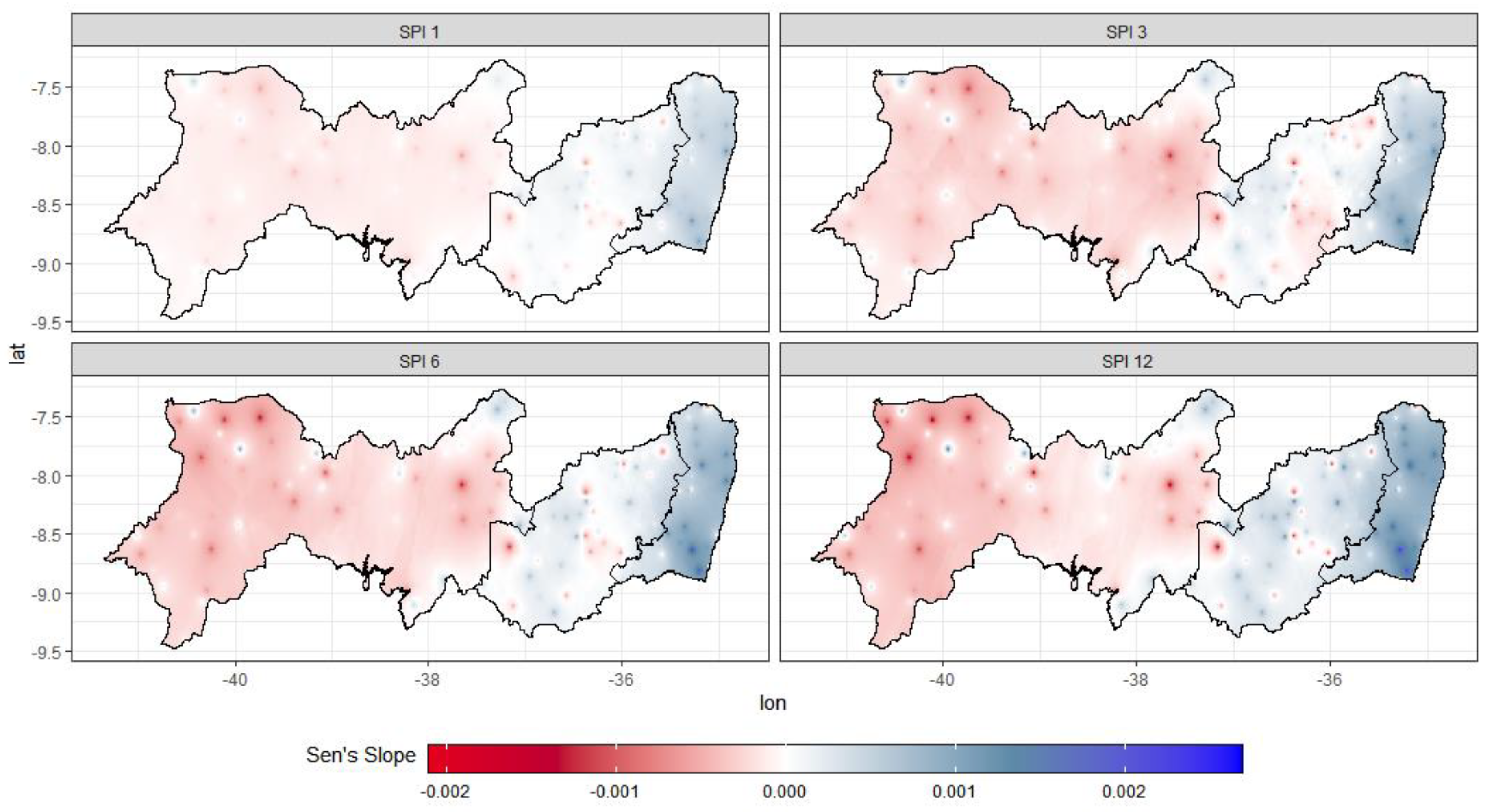
The spatial distribution of the magnitude of SPI trend (Sen’s slope) is shown in Figure 6. The signs of the slopes are consistent with the results of Mann–Kendall test: negative in Sertão, with decreasing magnitude from west to east towards the transitional Agreste region, where the trend becomes positive with increasing magnitude towards Zona de Mata. It is also seen that the Sen’s slope increases with the increase in aggregation time scale.
In order to assess the difference in trend magnitudes between each of the regions, we construct boxplots of SPI’s Sen’s slopes and perform the Wilcoxon–Mann–Whitney test at the 5% significance level (Figure 7). For all time scales the Sertão region has negative Sen’s slope, the Agreste region has a slightly positive Sen’s slope, and Zona da Mata has a high positive Sen’s slope. The test results indicate that there is a significant difference between the regions for all time scales.

3.2. Detrended Fluctuation Analysis

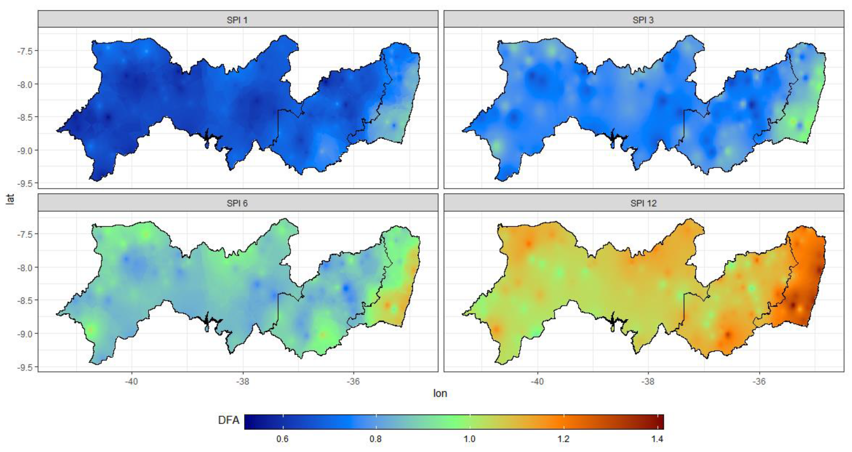
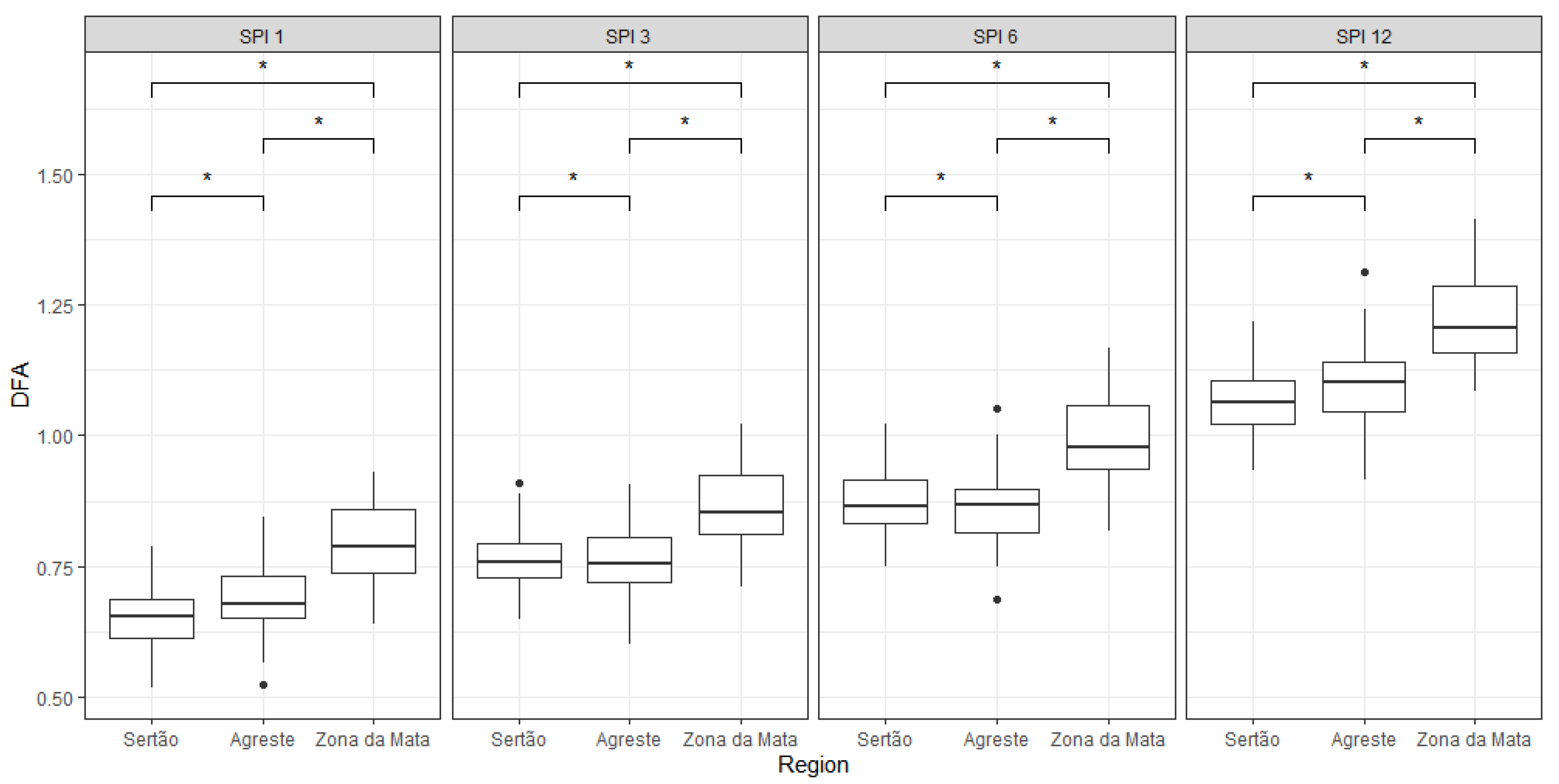
We apply DFA analysis on SPI time series for all the 133 Pernambuco stations, and perform spatial interpolation of obtained scaling exponents, resulting in maps shown in Figure 8. The values of DFA exponents are greater than 0.5 and increase with SPI time scale, indicating stronger persistency and higher predictability of medium-term conditions in precipitation (SPI-3 and SPI-6), while for short-term conditions described by SPI-1, the DFA exponent is closer to 0.5 indicating weak persistency and low predictability. Long-term precipitation patterns described by SPI-12, show different behavior: in Sertão and Agreste, the values of DFA exponents are around 1, indicating strong persistency, while in Zona da Mata the value of the DFA exponent is found to be between 1.0 and 1.5, indicating anti-persistent fractional Brownian motion (H = α − 1), meaning that SPI-12 increments exhibit anti-persistent long-term correlations. It can also be observed from Figure 6 that for short and medium conditions (SPI-1, SPI-3 and SPI-6), DFA exponents increase with decreasing distance to the ocean, indicating the weakest persistence (lowest predictability) in Sertão, and the strongest persistence (highest predictability) in Zona da Mata. The results obtained by DFA provide information about the existence of long-term correlations (predictability) of dry/wet conditions at different accumulation scales and is useful for agricultural planning and water resource management in the region. The DFA box plots for each region and all accumulation scales are shown in Figure 9. The verification of a significant difference between the regions was performed using the Wilcoxon–Mann–Whitney test at the 5% significance level. The test results shown in Figure 9 demonstrate that there is a significant difference between DFA exponents of the regions on all time scales. Recently Adarsh et al. [58] applied multifractal detrended fluctuation analysis—MFDFA (which is a generalization of DFA method) on SPI series from 30 meteorological subdivisions of India. They found that SPI time series exhibit persistence properties, with stronger persistence for higher time scales. Tatli et al. [59] applied DFA on Palmer drought severity index (PDSI) from 212 meteorological stations in Turkey and found that the values of scaling exponents were between 0.5 and 1, indicating the persistence of meteorological drought, which varies across the region. Qualitatively, our results are similar to those reported in these studies.

4. Conclusions

We analyze temporal fluctuations of Standardized Precipitation Index (SPI) for the period from 1950 to 2012 (calculated from monthly rainfall records from 133 gauging stations located in Pernambuco state, Brazil) by using three complementary methods: the Mann–Kendall test, Sen’s slope, and detrended fluctuation analysis (DFA). The results are interpolated over the entire study area to investigate spatial distribution of trend and persistence of SPI time series at different time scales. Our main findings are: (i) for all time scales significant negative trends were obtained in the (deep inland) Sertão region (with decreasing magnitude from west to east) while significant positive trends are found in Agreste and Zona da Mata regions, with increasing magnitude towards the coast; (ii) SPI-1 series that describe short-term dry/wet conditions (related with meteorological types of drought along with short-term soil moisture and crop stress) exhibit values of DFA exponents close to 0.5, indicating weak persistency and low predictability, while for medium-term conditions (SPI-3 and SPI-6, which are related with medium-term soil moisture conditions and seasonal to medium-term trends in precipitation) DFA exponents are greater than 0.5 and increase with accumulation period, indicating stronger persistency and higher predictability; (iii) for SPI-12 series that describe long-term precipitation patterns which are relevant for streamflows, reservoir levels, and groundwater levels, the values of DFA exponents for Sertão and Agreste are around 1, indicating strong persistency, while in the coastal Zona da Mata region the value of the DFA exponent is found to be between 1.0 and 1.5, indicating anti-persistent fractional Brownian motion; (iv) for both trend and persistence of SPI, we find a significant difference between the regions. While trend analysis of SPI was extensively studied for different parts of the world, much less is known about persistent properties of dry/wet conditions, at different time scales. Our results should be useful for agricultural planning and water resource management in the NEB and indicate that more studies should be dedicated to investigate long-term correlations in temporal series of various drought indices, in order to deepen the understanding of long-term predictability of dry/wet conditions of regions that are most vulnerable to extreme climatic episodes.
In conclusion, in order to assess different aspects of the phenomenon, we use a suite of complementary methods that are capable of revealing both tendencies and persistence (predictability) of the SPI index, at different time scales, in a geographically explicit setting. Therefore, the current work should not be seen as just a local case study, but rather as a contribution to establishing guidelines for a multi-dimensional approach, that may be used in other regions of the world.

Author Contributions

Conceptualization, A.S.A.d.S., T.S. and B.S.; Data curation, A.S.A.d.S., R.S.C.M. and B.S.; Formal analysis, A.S.A.d.S.; Funding acquisition, A.S.A.d.S., M.C.F. and R.S.C.M.; Investigation, A.S.A.d.S., M.C.F., T.S. and B.S.; Methodology, A.S.A.d.S., M.C.F., T.S. and B.S.; Software, A.S.A.d.S. and B.S.; Supervision, R.S.C.M., T.S. and B.S.; Validation, A.S.A.d.S., M.C.F., R.S.C.M., T.S. and B.S.; Visualization, A.S.A.d.S. and T.S.; Writing—original draft, A.S.A.d.S., M.C.F., T.S. and B.S.; Writing—review and editing, R.S.C.M., T.S. and B.S. All authors have read and agreed to the published version of the manuscript.

Funding

This research was funded by the Brazilian agencies CNPq (Grants 307445/2018-6, 304497/2019-3, 441305/2017-2, 465764/2014-2), Facepe (Grants APQ-0296-5.01/17,APQ-0532-5.01/14, APQ-0498-3.07/17 ONDACBC) and Capes (Grant 88887.136369/2017-00).

Acknowledgments

The authors acknowledge support of Brazilian agencies CNPq, CAPES and Facepe through the following research grants: CNPq 307445/2018-6, 304497/2019-3, 441305/2017-2; INCT–MCTI/CNPq/CAPES/FAPs 465764/2014-2; Facepe APQ-0296-5.01/17, APQ-0532-5.01/14.

Conflicts of Interest

The authors declare no conflict of interest.

References

  1. Trnka, M.; Semerádová, D.; Novotný, I.; Dumbrovský, M.; Drbal, K.; Pavlík, F.; Vopravil, J.; Štěpánková, P.; Vizina, A.; Balek, J.; et al. Assessing the Combined Hazards of Drought, Soil Erosion and Local Flooding on Agricultural Land: A Czech Case Study. Clim. Res. 2016, 70, 231–249. [Google Scholar] [CrossRef] [Green Version]
  2. Kalantari, Z.; Ferreira, C.S.S.; Keesstra, S.; Destouni, G. Nature-Based Solutions for Flood-Drought Risk Mitigation in Vulnerable Urbanizing Parts of East-Africa. Curr. Opin. Environ. Sci. Health 2018, 5, 73–78. [Google Scholar] [CrossRef]
  3. Bond, N.R.; Lake, P.S.; Arthington, A.H. The Impacts of Drought on Freshwater Ecosystems: An Australian Perspective. Hydrobiologia 2008, 600, 3–16. [Google Scholar] [CrossRef] [Green Version]
  4. Patz, J.A. Hotspots in Climate Change and Human Health. BMJ 2002, 325, 1094–1098. [Google Scholar] [CrossRef] [PubMed] [Green Version]
  5. Chadwick, R.; Good, P.; Martin, G.; Rowell, D.P. Large Rainfall Changes Consistently Projected over Substantial Areas of Tropical Land. Nat. Clim. Chang. 2016, 6, 177–181. [Google Scholar] [CrossRef]
  6. Palmer, W.C. Keeping Track of Crop Moisture Conditions, Nationwide: The New Crop Moisture Index. Weatherwise 1968, 21, 156–161. [Google Scholar] [CrossRef]
  7. Shukla, S.; Wood, A.W. Use of a Standardized Runoff Index for Characterizing Hydrologic Drought. Geophys. Res. Lett. 2008, 35, L02405. [Google Scholar] [CrossRef] [Green Version]
  8. McKee, T.B.; Doesken, N.J.; Kleist, J. The relationship of drought frequency and duration to time scales. In Proceedings of the 8th Conference on Applied Climatology, American Meteorological Society, Anaheim, CA, USA, 17–22 January 1993. [Google Scholar]
  9. Vicente-Serrano, S.M.; Beguería, S.; López-Moreno, J.I. A Multiscalar Drought Index Sensitive to Global Warming: The Standardized Precipitation Evapotranspiration Index. J. Clim. 2010, 23, 1696–1718. [Google Scholar] [CrossRef] [Green Version]
  10. Svoboda, M.; Hayes, M.; Wood, D. Standardized Precipitation Index User Guide; (WMO-No. 1090); WMO-World Meteorological Organization: Geneva, Switzerland, 2012; Available online: www.wamis.org/agm/pubs/SPI/WMO_1090_EN.pdf (accessed on 10 August 2020).
  11. Du, J.; Fang, J.; Xu, W.; Shi, P. Analysis of Dry/Wet Conditions Using the Standardized Precipitation Index and Its Potential Usefulness for Drought/Flood Monitoring in Hunan Province, China. Stoch. Environ. Res. Risk Assess. 2013, 27, 377–387. [Google Scholar] [CrossRef]
  12. Buttafuoco, G.; Caloiero, T.; Coscarelli, R. Analyses of Drought Events in Calabria (Southern Italy) Using Standardized Precipitation Index. Water Resour. Manag. 2015, 29, 557–573. [Google Scholar] [CrossRef]
  13. Ashraf, M.; Routray, J.K. Spatio-Temporal Characteristics of Precipitation and Drought in Balochistan Province, Pakistan. Nat. Hazards 2015, 77, 229–254. [Google Scholar] [CrossRef]
  14. Caloiero, T. Drought Analysis in New Zealand Using the Standardized Precipitation Index. Environ. Earth Sci. 2017, 76, 569. [Google Scholar] [CrossRef]
  15. Li, W.; Fu, R.; Juárez, R.I.N.; Fernandes, K. Observed Change of the Standardized Precipitation Index, Its Potential Cause and Implications to Future Climate Change in the Amazon Region. Phil. Trans. R. Soc. B 2008, 363, 1767–1772. [Google Scholar] [CrossRef]
  16. Marengo, J.A.; Alves, L.M.; Alvala, R.C.S.; Cunha, A.P.; Brito, S.; Moraes, O.L.L. Climatic Characteristics of the 2010–2016 Drought in the Semiarid Northeast Brazil Region. An. Acad. Bras. Ciênc. 2018, 90 (Suppl. 1), 1973–1985. [Google Scholar] [CrossRef] [PubMed]
  17. Marengo, J.A.; Torres, R.R.; Alves, L.M. Drought in Northeast Brazil—Past, Present, and Future. Theor. Appl. Climatol. 2017, 129, 1189–1200. [Google Scholar] [CrossRef]
  18. Cunha, A.P.M.A.; Tomasella, J.; Ribeiro-Neto, G.G.; Brown, M.; Garcia, S.R.; Brito, S.B.; Carvalho, M.A. Changes in the Spatial-Temporal Patterns of Droughts in the Brazilian Northeast. Atmos. Sci. Lett. 2018, 19, e855. [Google Scholar] [CrossRef] [Green Version]
  19. Marengo, J.A.; Bernasconi, M. Regional Differences in Aridity/Drought Conditions over Northeast Brazil: Present State and Future Projections. Clim. Chang. 2015, 129, 103–115. [Google Scholar] [CrossRef]
  20. Debortoli, N.S.; Camarinha, P.I.M.; Marengo, J.A.; Rodrigues, R.R. An Index of Brazil’s Vulnerability to Expected Increases in Natural Flash Flooding and Landslide Disasters in the Context of Climate Change. Nat. Hazards 2017, 86, 557–582. [Google Scholar] [CrossRef]
  21. Brito, S.S.B.; Cunha, A.P.M.A.; Cunningham, C.C.; Alvalá, R.C.; Marengo, J.A.; Carvalho, M.A. Frequency, Duration and Severity of Drought in the Semiarid Northeast Brazil Region. Int. J. Climatol. 2018, 38, 517–529. [Google Scholar] [CrossRef]
  22. Silva, B.K.N.; Lucio, P.S. Characterization of Risk/Exposure to Climate Extremes for the Brazilian Northeast—Case Study: Rio Grande Do Norte. Theor. Appl. Climatol. 2015, 122, 59–67. [Google Scholar] [CrossRef]
  23. Lyra, G.B.; Oliveira-Júnior, J.F.; Gois, G.; Cunha-Zeri, G.; Zeri, M. Rainfall Variability over Alagoas under the Influences of SST Anomalies. Meteorol. Atmos. Phys. 2017, 129, 157–171. [Google Scholar] [CrossRef]
  24. Santos, C.A.G.; Brasil Neto, R.M.; da Silva, R.M.; dos Santos, D.C. Innovative Approach for Geospatial Drought Severity Classification: A Case Study of Paraíba State, Brazil. Stoch. Environ. Res Risk Assess. 2019, 33, 545–562. [Google Scholar] [CrossRef] [Green Version]
  25. Melo Santos, A.M.; Cavalcanti, D.R.; da Silva, J.M.C.; Tabarelli, M. Biogeographical Relationships among Tropical Forests in North-Eastern Brazil. J. Biogeogr. 2007, 34, 437–446. [Google Scholar] [CrossRef]
  26. Ranta, P.; Blom, T.; Niemela¨, J.; Joensuu, E.; Siitonen, M. The fragmented Atlantic rain forest of Brazil: Size, shape and distribution of forest fragments. Biodivers. Conserv. 1998, 7, 385–403. [Google Scholar] [CrossRef]
  27. Alvares, C.A.; Stape, J.L.; Sentelhas, P.C.; de Moraes Gonçalves, J.L.; Sparovek, G. Köppen’s Climate Classification Map for Brazil. Meteorol. Z. 2013, 22, 711–728. [Google Scholar] [CrossRef]
  28. Da Silva, A.S.A.; Stosic, B.; Menezes, R.S.C.; Singh, V.P. Comparison of Interpolation Methods for Spatial Distribution of Monthly Precipitation in the State of Pernambuco, Brazil. J. Hydrol. Eng. 2019, 24, 04018068. [Google Scholar] [CrossRef]
  29. R Core Team. R: A Language and Environment for Statistical Computing; R Foundation for Statistic Computing: Vienna, Austria, 2019; Available online: https://www.R-project.org (accessed on 10 August 2020).
  30. Thorsten Pohlert. Trend: Non-Parametric Trend Tests and Change-Point Detection. R Package Version 1.1.2. 2020. Available online: https://CRAN.R-project.org/package=trend (accessed on 10 August 2020).
  31. Hayes, M.; Svoboda, M.; Wall, N.; Widhalm, M. The Lincoln Declaration on Drought Indices: Universal Meteorological Drought Index Recommended. Bull. Am. Meteorol. Soc. 2011, 92, 485–488. [Google Scholar] [CrossRef] [Green Version]
  32. Svensson, C.; Hannaford, J.; Prosdocimi, I. Statistical Distributions for Monthly Aggregations of Precipitation and Streamflow in Drought Indicator Applications. Water Resour. Res. 2017, 53, 999–1018. [Google Scholar] [CrossRef] [Green Version]
  33. Stagge, J.H.; Tallaksen, L.M.; Gudmundsson, L.; Van Loon, A.F.; Stahl, K. Candidate Distributions for Climatological Drought Indices (SPI and SPEI). Int. J. Climatol. 2015, 35, 4027–4040. [Google Scholar] [CrossRef]
  34. Wu, H.; Svoboda, M.D.; Hayes, M.J.; Wilhite, D.A.; Wen, F. Appropriate Application of the Standardized Precipitation Index in Arid Locations and Dry Seasons. Int. J. Climatol. 2007, 27, 65–79. [Google Scholar] [CrossRef]
  35. Thom, H. Some Methods of Climatological Analysis; The World Meteorological Organization: Geneva, Switzerland, 1966; pp. 16–22. [Google Scholar]
  36. Abramowitz, M.; Stegun, I.A. Handbook of Mathematical Functions: With Formulas, Graphs, and Mathematical Table; Courier Corporation: North Chelmsford, MA, USA, 1965; Volume 55. [Google Scholar]
  37. Lloyd-Hughes, B.; Saunders, M.A. A Drought Climatology for Europe. Int. J. Climatol. 2002, 22, 1571–1592. [Google Scholar] [CrossRef]
  38. Mann, H.B. Nonparametric tests against trend. Econometrica. J. Econ. Soc. 1945, 13, 245–259. [Google Scholar]
  39. Kendall, M.G. Rank Correlation Methods; Charles Griffin: London, UK, 1975. [Google Scholar]
  40. Birsan, M.V.; Dumitrescu, A.; Micu, D.M.; Cheval, S. Changes in annual temperature extremes in the carpathians since AD 1961. Nat. Hazards 2014, 74, 1899–1910. [Google Scholar] [CrossRef]
  41. Gocic, M.; Trajkovic, S. Analysis of Changes in Meteorological Variables Using Mann-Kendall and Sen’s Slope Estimator Statistical Tests in Serbia. Glob. Planet. Chang. 2013, 100, 172–182. [Google Scholar] [CrossRef]
  42. Raziei, T.; Daryabari, J.; Bordi, I.; Pereira, L.S. Spatial Patterns and Temporal Trends of Precipitation in Iran. Theor. Appl. Climatol. 2014, 115, 531–540. [Google Scholar] [CrossRef]
  43. Nashwan, M.S.; Shahid, S. Spatial distribution of unidirectional trends in climate and weather extremes in Nileriver basin. Theor. Appl. Climatol. 2019, 137, 1181–1199. [Google Scholar] [CrossRef]
  44. Mann, H.B.; Whitney, D.R. On a test of whether one of two random variables is stochastically larger than the other. Ann. Math. Stat. 1947, 18, 50–60. [Google Scholar] [CrossRef]
  45. Wilcoxon, F. Individual comparisons by ranking methods. Biometrics 1945, 1, 80–83. [Google Scholar] [CrossRef]
  46. Sen, P.K. Estimates of the regression coefficient based on Kendall’s tau. J. Am. Stat. Assoc. 1968, 63, 1379–1389. [Google Scholar] [CrossRef]
  47. Fernandes, R.; Leblanc, S.G. Parametric (modified least squares) and non-parametric (Theil–Sen) linear regressions for predicting biophysical parameters in the presence of measurement errors. Remote Sens. Environ. 2005, 95, 303–316. [Google Scholar] [CrossRef]
  48. Chervenkov, H.; Slavov, K. Theil-Sen Estimator vs. Ordinary LeastSquares—Trend Analysis for Selected ETCCDI Climate Indices. Comptes Rendus Acad. Bulg. Sci. 2019, 72, 47–54. [Google Scholar] [CrossRef]
  49. Peng, C.-K.; Buldyrev, S.V.; Havlin, S.; Simons, M.; Stanley, H.E.; Goldberger, A.L. Mosaic Organization of DNA Nucleotides. Phys. Rev. E 1994, 49, 1685–1689. [Google Scholar] [CrossRef] [PubMed] [Green Version]
  50. Hu, K.; Ivanov, P.C.; Chen, Z.; Carpena, P.; Stanley, H.E. Effect of Trends on Detrended Fluctuation Analysis. Phys. Rev. E 2001, 64, 011114. [Google Scholar] [CrossRef] [PubMed] [Green Version]
  51. Chen, Z.; Ivanov, P.C.; Hu, K.; Stanley, H.E. Effect of Nonstationarities on Detrended Fluctuation Analysis. Phys. Rev. E 2002, 65, 041107. [Google Scholar] [CrossRef] [PubMed] [Green Version]
  52. Goldberger, A.L.; Amaral, L.A.N.; Hausdorff, J.M.; Ivanov, P.C.; Peng, C.-K.; Stanley, H.E. Fractal Dynamics in Physiology: Alterations with Disease and Aging. Proc. Natl. Acad. Sci. USA 2002, 99 (Suppl. 1), 2466–2472. [Google Scholar] [CrossRef] [Green Version]
  53. Currenti, G.; Negro, C.; Lapenna, V.; Telesca, L. Fluctuation Analysis of the Hourly Time Variability of Volcano-Magnetic Signals Recorded at Mt. Etna Volcano, Sicily (Italy). Chaos Solitons Fractals 2005, 23, 1921–1929. [Google Scholar] [CrossRef]
  54. Kiraly, A.; Janosi, I.M. Detrended Fluctuation Analysis of Daily Temperature Records: Geographic Dependence over Australia. Meteorol. Atmos. Phys. 2005, 88, 119–128. [Google Scholar] [CrossRef] [Green Version]
  55. De Oliveira Santos, M.; Stosic, T.; Stosic, B.D. Long-Term Correlations in Hourly Wind Speed Records in Pernambuco, Brazil. Phys. A Stat. Mech. Appl. 2012, 391, 1546–1552. [Google Scholar] [CrossRef] [Green Version]
  56. Telesca, L.; Lovallo, M.; Lopez-Moreno, I.; Vicente-Serrano, S. Investigation of Scaling Properties in Monthly Streamflow and Standardized Streamflow Index (SSI) Time Series in the Ebro Basin (Spain). Phys. A Stat. Mech. Appl. 2012, 391, 1662–1678. [Google Scholar] [CrossRef]
  57. Yamasaki, K.; Muchnik, L.; Havlin, S.; Bunde, A.; Stanley, H.E. Scaling and Memory in Volatility Return Intervals in Financial Markets. Proc. Natl. Acad. Sci. USA 2005, 102, 9424–9428. [Google Scholar] [CrossRef] [Green Version]
  58. Adarsh, S.; Kumar, D.N.; Deepthi, B.; Gayathri, G.; Aswathy, S.S.; Bhagyasree, S. Multifractal Characterization of Meteorological Drought in India Using Detrended Fluctuation Analysis. Int. J. Climatol. 2019, 39, 4234–4255. [Google Scholar] [CrossRef]
  59. Tatli, H.; Dalfes, H.N. Long-Time Memory in Drought via Detrended Fluctuation Analysis. Water Resour. Manag. 2020, 34, 1199–1212. [Google Scholar] [CrossRef]
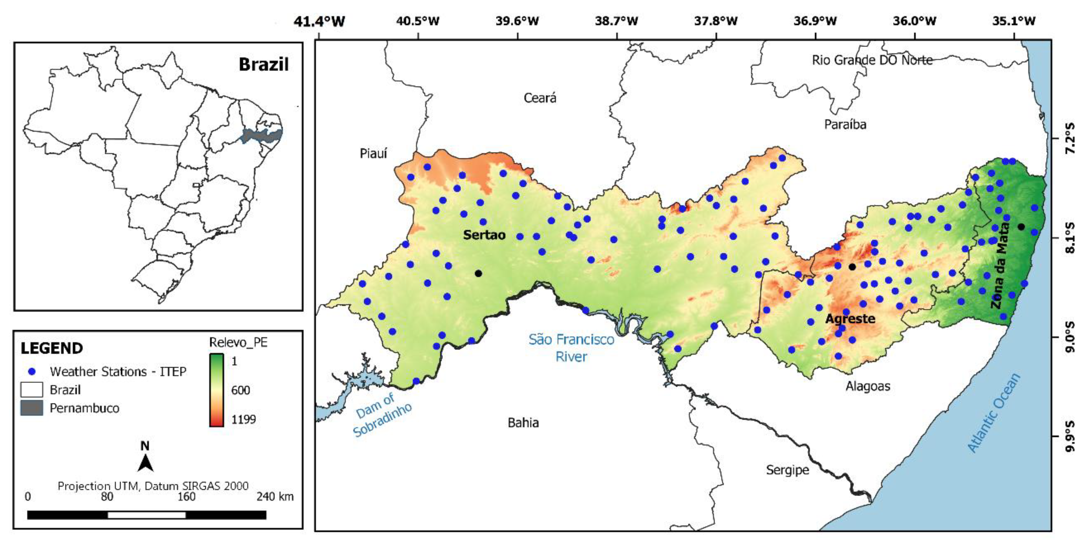
Figure 1. Geographical location of the state of Pernambuco, Brazil, and the spatial arrangement of the ITEP weather stations, with incorporated topographic information.
Atmosphere 11 01134 g001
Figure 2. Mean annual precipitation, interpolated over the study area.
Atmosphere 11 01134 g002
Figure 3. Monthly precipitation (a) and SPI values (b) at different time scales (SPI-1, SPI-3, SPI-6 and SP-12), for representative stations of the three regions.
Atmosphere 11 01134 g003
Figure 4. Results of the trend analysis for SPI at different time scales (SPI-1, SPI-3, SPI-6 and SP-12).
Atmosphere 11 01134 g004
Figure 5. Spatial distribution of the SPI trend over Pernambuco state, at a significance level of 0.05. Filled triangles indicate significant trends, as obtained by Mann–Kendall test.
Atmosphere 11 01134 g005
Figure 6. Spatial distribution of Sen’s slope, interpolated across the Pernambuco state.
Atmosphere 11 01134 g006
Figure 7. Sen’s slope boxplots for each of the three regions for different time scales (SPI-1, SPI-3, SPI-6 and SPI-12). The star symbol “*” indicates that there is a significant difference between the regions at the 5% significance level ( p v < 0.05 ).
Atmosphere 11 01134 g007
Figure 8. Spatial distributions of detrended fluctuation analysis (DFA) exponents α for SPI at different time scales (SPI-1, SPI-3, SPI-6 and SPI-12) across Pernambuco state.
Atmosphere 11 01134 g008
Figure 9. DFA exponents α boxplots for each region for SPI at different time scales (SPI-1, SPI-3, SPI-6 and SPI-12). The star symbol “*” indicates that there is a significant difference between the regions at the 5% significance level ( p v < 0.05 ).
Atmosphere 11 01134 g009
Table 1. Dry/wet categories defined by [8]. SPI: Standardized Precipitation Index.
SPI ClassificationSPI Value
Extremely dry S P I < 2
Severely dry 2 S P I < 1.5
Moderately dry 1.5 S P I < 1.0
Near Normal 1.0 S P I < 1.0
Moderately wet 1.0 S P I < 1.5
Very wet 1.5 S P I < 2.0
Extreme wet S P I 2.0
Publisher’s Note: MDPI stays neutral with regard to jurisdictional claims in published maps and institutional affiliations.