The Influence of Land Surface Temperature in Evapotranspiration Estimated by the S-SEBI Model

Abstract

Evapotranspiration (ET) is one of the least understood components of the hydrological cycle. Its applications are varied, from agricultural, ecological and hydrological monitoring, to control of the evolution of climate change. The goal of this work was to analyze the influence that uncertainties in the estimate of land surface temperature (Ts) can cause on ET estimates by S-SEBI model in the Pampa biome area. Also, the specificities of native grassland of Pampa biome related to energy balance were analyzed. The results indicate that the daily evapotranspiration is higher when the pixel Ts is lower, which also shows the influence of land use on the variability of ET. The results demonstrated that the S-SEBI is less dependent on Ts estimation than other models reported in the literature, such as the SEBS, which not exceed 0.5 mm/day in grasslands. The evapotranspiration variability between forest and grassland were lower than expected, demonstrating that the Pampa biome have in Rio Grande do Sul the same importance that forests regarding to the processes of the hydrological cycle, since it covers 63% of the State.

1. Introduction

The physical, chemical and biological processes responsible for life on Earth depend practically on solar energy. Monitoring energy and soil-vegetation-atmosphere mass transfers is a key step in the management of water and agricultural resources, with different applications depending on the spatial and temporal scales of interest. It is also useful for a better understanding and prediction of climate evolution [1,2].

There are two ways of thinking about evapotranspiration: (1) hydrologically, in which ET is what is loss of water in the hydrological cycle by the plants; In this sense, precipitation, subsurface runoff, surface runoff, and evapotranspiration should also be taken into consideration [2]; (2) energetically, when considering the energy used for the process of water loss by the plants to the atmosphere by determining the magnitude of radioactive and non-radiative fluxes [1,3]. The radiation balance represents the energy available by the system to non-radiative process, such as evaporate of water or evapotranspiration on vegetated surfaces, by the latent heat flux (LE), heat the atmosphere by the sensible heat flux (H) and heat the subsoil by soil heat flux (G) [1,4,5].

Land surface temperature (Ts) is one of the sources of input data for modelling land surface processes, such as actual and potential evapotranspiration (ET) that is a critical component of many agricultural and ecological studies [3,6,7,8]. The identification of the uncertainties resulting from the different input variables in the estimation of ET remains a challenge due to the complexity of the parameterization of the models [9,10].

Many studies estimate that 60% of the precipitated water returns to the atmosphere through evapotranspiration [1,3,7,11]. However, the ET is one of the least understood components of the hydrological cycle [1,3]. Conventional measurements of ET (lysimeter data, eddy covariance, Bowen ratio) have limited application because they are not spatially representative and because of the dynamic’s nature of heat transfer processes, also its accuracy is significantly degraded when attempts are made to interpolate or extrapolate spatially sparse measurement networks to landscape and regional scales [12]. Therefore, remote sensing analyses could be an alternative to solve these problems by different methods, which obtaining large-scale ET, ranging from individual pixels to an entire raster image. Algorithms have been developed utilizing information from different meteorological and atmospheric input variables (MOD16, SEBAL, S-SEBI, SEBS, SSEB, SEBTA, SAFER) [3,13,14,15].

The Simplified Surface Energy Balance Index (S-SEBI) model estimates evapotranspiration from the relationship between Ts and albedo, since it calculates the evaporative fraction by defining the temperatures in drier and wetter regions [8,16,17,18]. Hence, the estimation of Ts is an important step for the proper functioning of this model. Abid et al. [10] tested the sensitivity of SEBS model to the uncertainties of various input data and their results show that the changes of ET reach 2 mm/day for changes in Ts.

Gibson et al. [9] discussed the complexities associated with derivation of ET and the uncertainties related to data and models that have implied potential errors at various stages of ET estimation. These errors are related to two situations: (1) error production and (2) error propagation. Error production refers to a situation where errors in the output products are mainly assigned to the specific operations applied to the data, thus producing errors in the ETs while there were no errors in the original data used as input. Error propagation refers to the process where potentially incorrect input data is passed through certain processing sequences and errors accumulate in ET output.

This study was performed in Pampa biome, which is a permanent grassland ecosystem occupied mostly by human activities as livestock and annual crops. Nowadays, the Pampa biome is the most altered, most threatened and least protected biome on the planet, which is the price it pays for having been, since the most remote historical times, one of the most favorable environments to the human establishment and also one of the most productive [19,20]. In order to sustain national measures to protect the biodiversity of this biome, it is understood that investments in local research of its particularities are necessary [21] and therefore this work also focuses on the singularities of the native vegetation of the biome concerning the energy balance.

The main objective of this work was to analyse the influence that the uncertainties in the estimate of Ts can cause on daily ET estimates by S-SEBI model, we evaluated the model with eddy-covariance measurements in a native grassland area in Southern Brazil (the Pampa biome). The impact that contrasting native grassland particularities related to energy balance were analyzed and compared with Forest and Exposed Soil. This is the first study of its kind in this region.

2. Materials and Methods

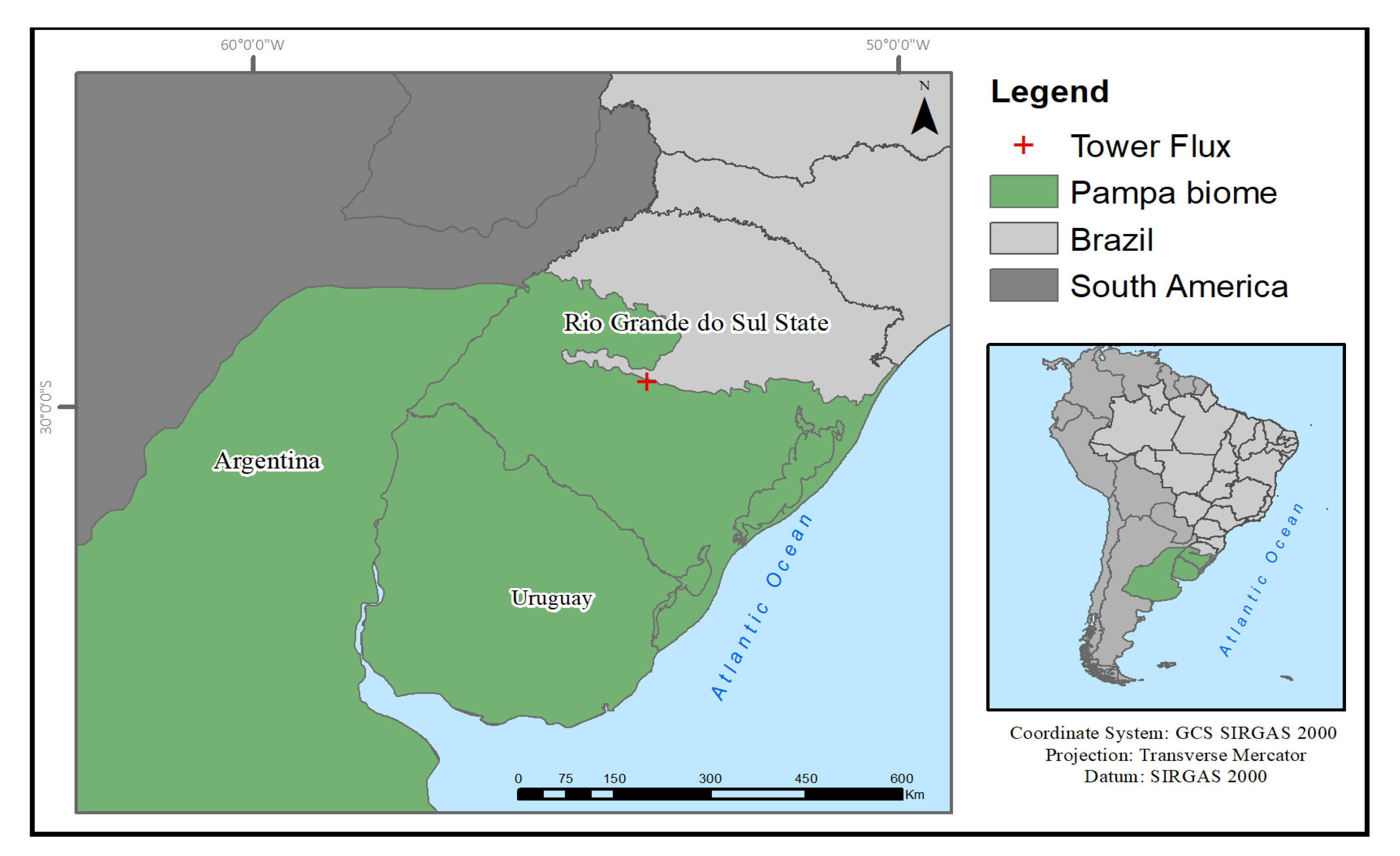
2.1. Study Area

The Pampa biome is considered by the Ministério do Meio Ambiente (MMA/Brazil) as one of the most important temperate field areas on the planet. In South America, this biome extends over an area of approximately 750,000 km², shared by Brazil, Uruguay and Argentina. In Brazil, this biome is restricted to 63% of the State of Rio Grande do Sul (RS) and represents 2.07% of the national territory.

From the point of view of biodiversity and environmental services, the fields are a fodder source for cattle ranching, shelter diversity of plant and animal species, and ensure the conservation of water resources [22]

The experimental site is located in the Federal University of Santa Maria (UFSM), covering 24 ha of natural vegetation (native grassland) belong to Pampa biome (Figure 1). This study area is part of the International Long Term Ecological Research (ILTER) network and is used for experiments in several areas of knowledge, mainly focused on the morphology of native species for livestock production [23,24].

2.2. Simplify Surface Energy Balance Index (S-SEBI)

The estimation of evapotranspiration from remote sensing data uses thermal infrared (TIR) sensors on satellite, which is based on assessing the energy balance through several surface properties such as albedo, vegetation cover and surface temperature [3]. When considering instantaneous conditions, the surface energy balance is obtained by determining the magnitude of the radiative and non-radiative fluxes the energy balance is written as:

LE = Rn − G − H

(1)

where LE is the latent heat flux of evaporation or evapotranspiration due to ET; Rn is the surface net radiation; H is the sensible heat flux; and G is the soil heat flux. The variables are expressed in energy units (W/m²). ET in volume units (e.g., liters m⁻² d⁻¹, usually simplified to mm d⁻¹ to express ET as a depth of water over an indefinite area) can be calculated from LE by the amount of energy needed to evaporate water at a specific temperature and pressure⁶².

Once the surface energy balance equation is discriminated, the Rn is calculated as the rest term of all incoming and outgoing shortwave (sw) and longwave (lw) radiation, as describing below:

$$\mathrm{Rn}=\left(1-\mathsf{\alpha }\right)\mathrm{Rs}\downarrow + \mathsf{\epsilon }\mathrm{RL}\downarrow -{ \mathsf{\epsilon }\mathsf{\sigma }\mathrm{Ts}}^4$$

(2)

where Rs (W/m²) is the shortwave downward radiation; RL (W/m²) is the longwave downward radiation; α is the surface albedo; ε is the surface emissivity; Ts (K) is the land surface temperature and σ is the Steffan-Boltzmann constant (5.67 × 10⁻⁸ W m⁻² K⁻⁴).

The latent heat flux (LET) depends on the evaporative fraction (Λ) and is given as follows:

LET = Λ (Rn − G)

(3)

The evaporative fraction concept (Λ) was proposed by [16], adapted and tested by [8,18], and it is described by the equation below:

Λ = (T_H − Ts)/(T_H − T_LE)

(4)

where T_H (K) is the temperature corresponding to dry condition and T_LE (K) is the temperature corresponding to wet condition.

This method can be only applied when the atmospheric conditions are constants over the image and the study site includes simultaneously wet and dry areas [8,16,18]. Besides of that, this method works better in a homogeneous vegetated area - with higher variance between dry and wet pixels.

2.3. Daily Evapotranspiration

Remote sensing data provides instantaneous radiation measurements. However, for agriculture and environment applications the evapotranspiration values are more useful. So, daily ET is defined as the temporal integration of ET instantaneous values in a day. The daily ET can be obtained using the Cdi, which consists of the ratio between the daily net radiation flux (Rnd) and instantaneous radiation flux (Rni), both from the tower flux. This concept was also adopted by Gómez et al. (2005) and Sobrino et al. [17,18]. Thus, Cdi was calculated through the integration of the radiation for the whole day:

Cdi = Rnd/Rni

(5)

Afterwards, the daily ET (mm/day) can be written as follows:

ET = (Λ Rn Cdi) 0.035265

(6)

where the soil heat flux (G) was not included according to [25] assuming that much of the energy that enters the soil during the day returns to the atmosphere at night through terrestrial longwave radiation.

2.4. Data Used in the Model

In this section the inputs used in this study, including satellite and meteorological data, are presented.

Table 1. Information of satellite and meteorological data to each variable calculated.

Data	Source (Online)	Spatial Resolution	Variable Calculated
Landsat 8 OLI	Earth Explorer-USGS	30 m	NDVI, α, ε
Landsat 8 TIRS		100 m	Ts
Air temperature (Ta)	INMET-SANTA MARIA (83936)		w
Atmospheric pressure (P)		local
Relative humid (RH)
Shortwave downward radiation (RS)	NCEP-CFSv2	0.205-horizontal resolution	Rn
longwave downward radiation (RL)

shows the information about resolution, data source and variables calculated, they are all explained in the subsections.

2.4.1. Satellite Data

Landsat 8 has two sensors which operated simultaneously and independently: (1) the Operational Land Imager (OLI) and (2) the Thermal Infrared Sensor (TIRS). The OLI images from visible to short-wave infrared and TIRS has thermal images of two-channels [26]. We acquired 22 cloud free Landsat 8 OLI and TIRS images, from 2015 and 2019, for the temporal and comparative analysis, the images passage occurs at 13:25 UTC. A Landsat 8 scene size is 185 km × 180 km, however the images were cut to a mask covering the study area, where the flux tower is located, covering mostly by a native vegetation of the Pampa biome with controlled cattle management.

Table 2. Information of the Landsat 8 OLI/TIRS scenes used in this study, Path/Row (222/81).

Acquisition Date	DOY	Season	Cloud Cover (%)
20 March 2015	78	Autumn	7.56
07 May 2015	126	Autumn	0.02
27 August 2015	238	Winter	20.58
12 September 2015	254	Winter	0.03
28 September 2015	270	Spring	4.22
15 November 2015	318	Spring	6.08
18 January 2016	17	Summer	0.00
28 July 2016	209	Winter	28.58
13 August 2016	225	Winter	19.8
03 October 2017	275	Spring	0.76
20 November 2017	323	Spring	0.49
22 December 2017	355	Summer	6.38
29 April 2018	118	Autumn	27.9
16 June 2018	166	Autumn	7.12
18 July 2018	198	Winter	12.53
25 December 2018	358	Summer	7.85
26 January 2019	25	Summer	4.14
18 May 2019	137	Autumn	0.89
19 June 2019	169	Autumn	1.13
21 July 2019	201	Winter	0.01
06 August 2019	217	Winter	0.01
09 October 2019	281	Spring	0.49

shows all days of the years and the season of the images used in this study.

The Landsat data cover 185 km × 180 km Level 1 terrain-corrected products, in which the spatial resolution of TIRS bands are 100 m and resampled by cubic convolution to 30 m to be co-registered with the 30 m OLI spectral bands [27]. Also, Landsat 8 OLI surface reflectance Level-2 products are generated at the Earth Resources Observation and Science (EROS). The EROS Science Processing Architecture (ESPA) on-demand interface corrects satellite images for atmospheric effects to create Level-2 data products. These Level 2 products were used in this research to obtain the normalized difference vegetation index (NDVI) and surface albedo.

2.4.2. Meteorological Data

Two meteorological databases were used to produce Rn and Ts of this study: (1) The Brazilian Meteorological Institute (Instituto Nacional de Meteorologia-INMET), located in Santa Maria city near 4 km from the study area, has provided: air temperature (Ta), atmospheric pressure (P) and relative humid (RH); (2) The National Centers for Environmental Prediction Climate (NCEP) Forecast System Version 2 (CFSv2) has provided reanalysis data, including the shortwave downward radiation (R_S) and longwave downward radiation (R_L). All the meteorological data were acquired to coincide with the time and date of the satellite passage.

We extracted the reanalysis data from the CFSv2 hourly product. The parameters were obtained with 0.205° horizontal resolution for an average between 13–14 h UTC on selected dates. From INMET the data were acquired at 12 UTC on the same selected dates. The solar radiation does not vary too much in two hours, so it is assumed the variation of the instantaneous measurements in this small period is not significant [7,16].

2.5. Variables Input of S-SEBI

To estimate the balance energy by remote sensing models some pre-processing of image data are needed and some surface properties had to be calculated.

Table 3. Equations applied to Landsat-8 data.

Variable	Equation	Description
NDVI	$\frac{\rho NIR-\rho RED}{\rho NIR+\rho RED}$	$\rho$ NIR is the Near Infrared reflectance of Landsat 8 (0.86 µm) and $\rho$ RED refers to the Red band reflectance of Landsat 8 OLI and (0.65 µm) [28]
A	$0.13{\rho }_1+0.115{\rho }_2+0.143{\rho }_3+0.18{\rho }_4+0.281{\rho }_5+0.108{\rho }_6+0.042{\rho }_7$	ρ is the reflectance at each Landsat 8 OLI channel [29]
Ts	$Ti+1.378\left(Ti-Tj\right)+0.183{\left(Ti-Tj\right)}^2-0.268+\left(54.3-2.238w\right)\left(1-\epsilon \right)+\left(-129.2+16.4w\right)$;	Ti and Tj are the at-sensor brightness temperatures at the bands i (10) and j (11) in Kelvins; ε is the mean emissivity, ε = 0.5 (εi + εj), Δε is the emissivity difference, Δε = (εi − εj); w is the total atmospheric water vapor content (in g/cm−2) [26,30]
W	$w_0 x RH x 0.098$	Water vapor (in g/cm−2); [31]; where RH is relative humid (%)
w0	$1.0007+3.46 \left({10}^{-6}P\right) {6.1121}^{17502\frac{Ta}{\left(240.97+Ta\right)}}$	P is atmospheric pressure (mb) and Ta is air temperature (Celcius)
ε	$a+b\rho RED;\left(FVC=0\right)$ ${\epsilon }_s\left(1-FVC\right)+{\epsilon }_{v}FVC;(0<FVC<1)$ $\epsilon =0.99;\left(\mathrm{FVC}=1\right)$	FVC is the Fractional Vegetation Cover and is given by FVC = NDVI − NDVIs/NDVIv − NDVIs; εs and εv are the soil and vegetation emissivity values respectively [32]
Soil Heat Flux (G)	$\left(\left(\frac{T_s}{\alpha }\right)\times \left(0.0038\times \alpha \right)+\left(0.0074 {\alpha }^2\right)\times \left(1-0.98\times NDV{I}^4\right)\right)\times Rn$	[33]

shows the algorithms used to calculate Normalized Difference Vegetation Index (NDVI), Albedo (α), Soil Heat Flux (G), Land Surface Temperature (Ts), which is dependent on water vapor (w), and Land Surface Emissivity (ε). All these variables were calculated for the whole study area by remote sensing process.

2.6. Land Surface Temperature of S-SEBI Model

To analyze the influence that possible uncertainties in the estimation of Ts may have on the estimates of LET, a noise was applied to the Ts images, with a Gaussian variation of −2 K and +2 K. Many authors believe that Ts retrieval precision varies around 1–2 K depending on the heterogeneity atmospheric conditions and the resolution of the sensor used in the process [26,34,35,36].

It is important to emphasize that, with this noise, the average Ts of the images does not vary, but the minimum and maximum temperatures do, as we can see in

Table 4. Land Surface Temperature stats of the images.

DOY	Average	Min	Min *	Max	Max *
78	306.68	302.88	300.28	315.66	317.63
126	292.18	289.41	287.27	295.89	298.33
238	295.16	293.35	290.84	297.85	300.04
254	292.82	288.85	287.34	295.97	298.27
270	300.09	295.25	293.67	305.98	306.79
318	303.27	298.64	297.31	308.68	310.52
17	310.67	298.67	297.23	323.209	325.068
209	287.41	284.77	282.97	290.48	293.037
225	294.04	290.46	288.57	298.381	300.38
275	298.41	294.98	293.03	301.437	303.466
323	310.17	302.73	300.62	320.88	321.847
355	311.41	303.47	302.15	320.889	321.532
118	301.04	296.82	295.25	305.507	307.662
166	284.88	281.68	279.92	288.066	290.438
198	296.68	294.71	292.3	298.152	301.019
358	305.54	301.55	299.52	311.657	313.422
137	295.52	292.28	290.41	297.604	299.857
169	291.57	288.96	286.92	293.546	296.418
201	297.32	295.28	292.42	300.20	302.042
217	294.43	292.37	289.95	296.84	299.462
281	303.99	299.38	298.12	309.80	311.864

* with noise on Land Surface Temperature.

.

2.7. Validation

2.7.1. Eddy-Covariance (EC) Data and Flux Tower

The estimated energy balance fluxes were compared with EC measurements in the experimental site, evaluating the model performance by regression analysis. The experimental surface fluxes data were obtained with a flux towers installed in the experimental site at (29.725° S; 53.760° W). For turbulent fluxes, the sensor set included a 3D sonic anemometer (Wind Master Pro; Gill Instruments, Hampshire, UK), measuring wind and air temperature components, and a gas analyzer (LI7500, LI-COR Inc., Lincoln, NE, USA), measuring the H₂O/CO₂ concentration at 3-m height sampled at a 10-Hz frequency, from 1 September 2014 to 15 June 2016. After this period, the gas analyzer and the anemometer were replaced by the sensor Integrated CO₂ and H₂O Open-Path Gas Analyzer and a 3D Sonic Anemometer (IRGASON, Campbell Scientific Inc., Logan, UT, USA). The net radiation was measured at 3-m height with a net radiation sensor (CNR4, Kipp & Zonen, Delft, The Netherlands) and the soil heat flux was measured with soil heat plates (HFP01, Hukseflux Thermal Sensors B.V., Delft, The Netherlands) placed at 0.10-m depth.

The eddy covariance, EC, Aubinet et al. method [37] was used in the high-frequency data (10 Hz) for the determination of latent heat flux (LE) and sensible heat flux, both turbulent fluxes, over 30-min block average using EddyPro^® software version 6.1 (LI-COR). with the configurations described in [7]. The footprint analyses of the EC data by Kljun et al. [38] indicates that about 90% of the flux originated within a circle with a radius of 115 m centered in the flux tower.

The daily mean of the fluxes was used to close the energy balance throughout the Bowen ratio approach [39], generating a corrected LE. More details about the experimental site and flux data processing are described in Rubert et al. [7]. We have evaluated experimental flux data in days with clear sky conditions between 2014 and 2019 and only in dates with less than 2 h missing data.

2.7.2. Statistical Analyses

To assess the model’s accuracy and to compare the model with and without the noise applied, we used the ratio of estimated and observed values, coefficient of determination (r²), mean bias error (Bias) (Equation (7)), root mean square error (RMSE) (Equation (8)), and mean standard deviation (MSD) (Equation (9). RMSE is the overall error in the predictions relative to the actual measured value, while MAE measures the average magnitude of the errors in a set of predictions (without considering their direction), and r² determines the strength of the linear relationship between estimates and measurements [40,41]. Furthermore, we used the Student’s t-test (with a 95% confidence level) to evaluate the significance of the linear relationship between observed and estimated values [41,42]

Bias = Σ (Oi − Pi)/n

(7)

$$\mathrm{RMSE} = \surd \frac{1}{\mathrm{n}} {\displaystyle \sum } (\mathrm{Pi}-\mathrm{Oi}{)}^2$$

(8)

$$\mathrm{MSD} = \sqrt{\frac{1}{\mathrm{N}-1}{\displaystyle \sum }_{\mathrm{i} = 1}^{\mathrm{N}}{({\mathrm{O}}_{\mathrm{i}}-\overline{\mathrm{x}})}^2}\frac{1}{\mathrm{n}}$$

(9)

3. Results

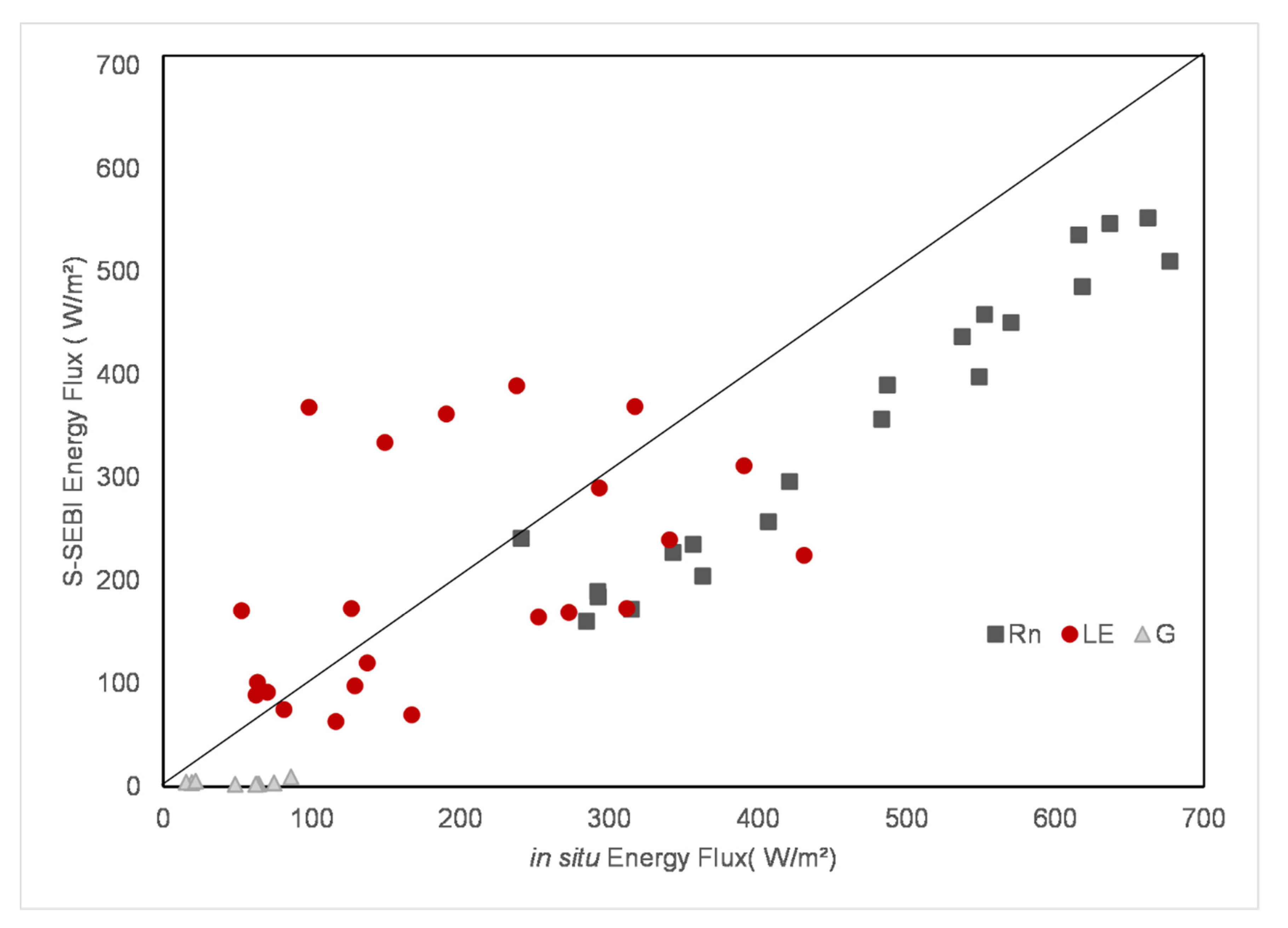
3.1. S-SEBI Validantion

The energy balance components estimated with S-SEBI and in situ measurements are shown in Figure 2 considering all scenes available.

The net radiation (Rn) measurements are the most accurate measurements of all the components in the surface energy budget, and they represent the largest part of the global radiation [39]. We have found a strong coefficient of correlation (0.81), the data produced the worst estimates of RMSE and Bias, with 138.7 (W/m²) and 132.12 (W/m²), respectively. Those results may be influencing the results of LE, because when Rn reaches more than 350 W/m² the latent heat flux tend to deviate. Besides of that, some authors have discussed that in days with no clouds and Rn less than 200 W/m² (mostly during the winter season) the model represents better all the fluxes [7]. Schirmbeck et al. [43] obtained a RMSE of 50 (W/m²), and Silva Oliveira et al. [44] testing METRIC model in Brazilian Cerrado obtained a RMSE of 59.8 (W/m²) with an overestimation of 9%.

The soil heat flux (G) is responsible for lower energy consumption, representing less than 10% in studied in pampa biome [43,45,46]. The model used in our study to produced G overestimate all the flux tower measurement, and they have produced the estimation of RMSE and Bias with 43.45 (W/m²) and 40.4 (W/m²), respectively. Gomis-Cebolla et al. [47] have validated four ET models, including SEBS in tropical forests of the Amazonian region, and they have concluded that their results serve to emphasize the need to improve the accuracy of reanalysis estimates in order to improve the accuracy in ET estimates. Therefore, the reanalysis data may be inserting minimums errors in our model as well.

According to Twine et al. [39] and Silva Oliveira et al. [44] LE tends to be underestimated by EC method due to sources of errors such as non-homogeneous surface coverage, soil characteristics, instrumental errors, topography, divergence or flux dispersion, among others. In LE analyzes, we have obtained mean errors (RMSE) around 92 (W/m²) and Bias 7.09 (W/m²), which agree with previous studies in Pampa biome of Schirmbeck et al. that obtained an overestimation of 94 (W/m²) testing OSEB and SEBAL models for 84 MODIS images between 2009–2011. Those uncertainties associated with derived LE could be caused especially because of the evaporative fraction component which is limited by the selection of dry and wet pixels [48]. A physically based two-source energy balance (TSEB) model was tested in an irrigated agricultural area in China applied to high resolution WiDAS data and ASTER data and compared with EC measurements, to LE the authors found Bias and RMSE as 113 W/m² and 140 W/m², respectively [12].

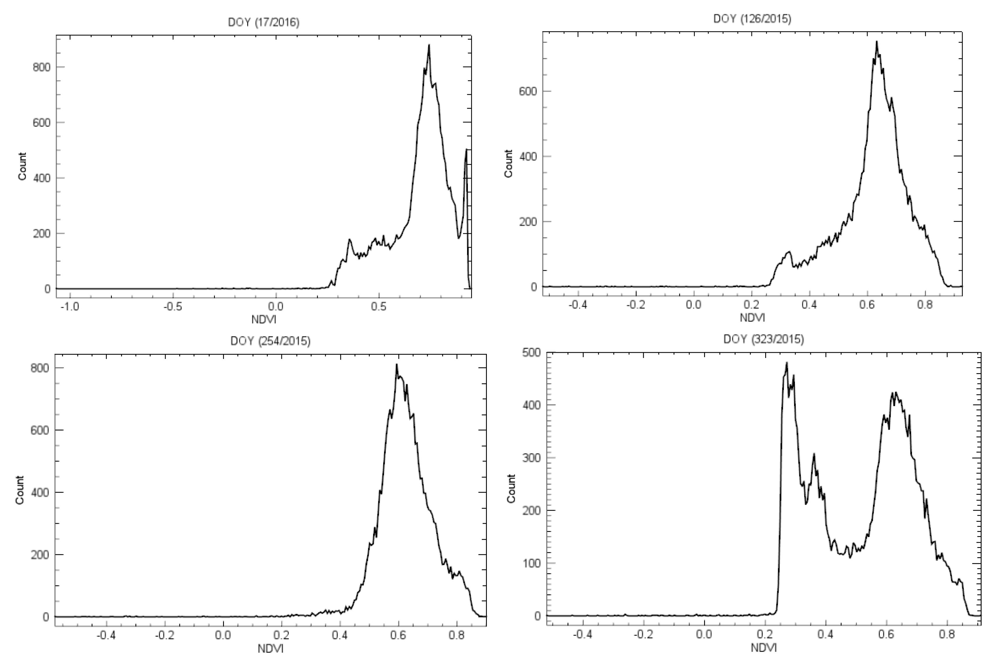
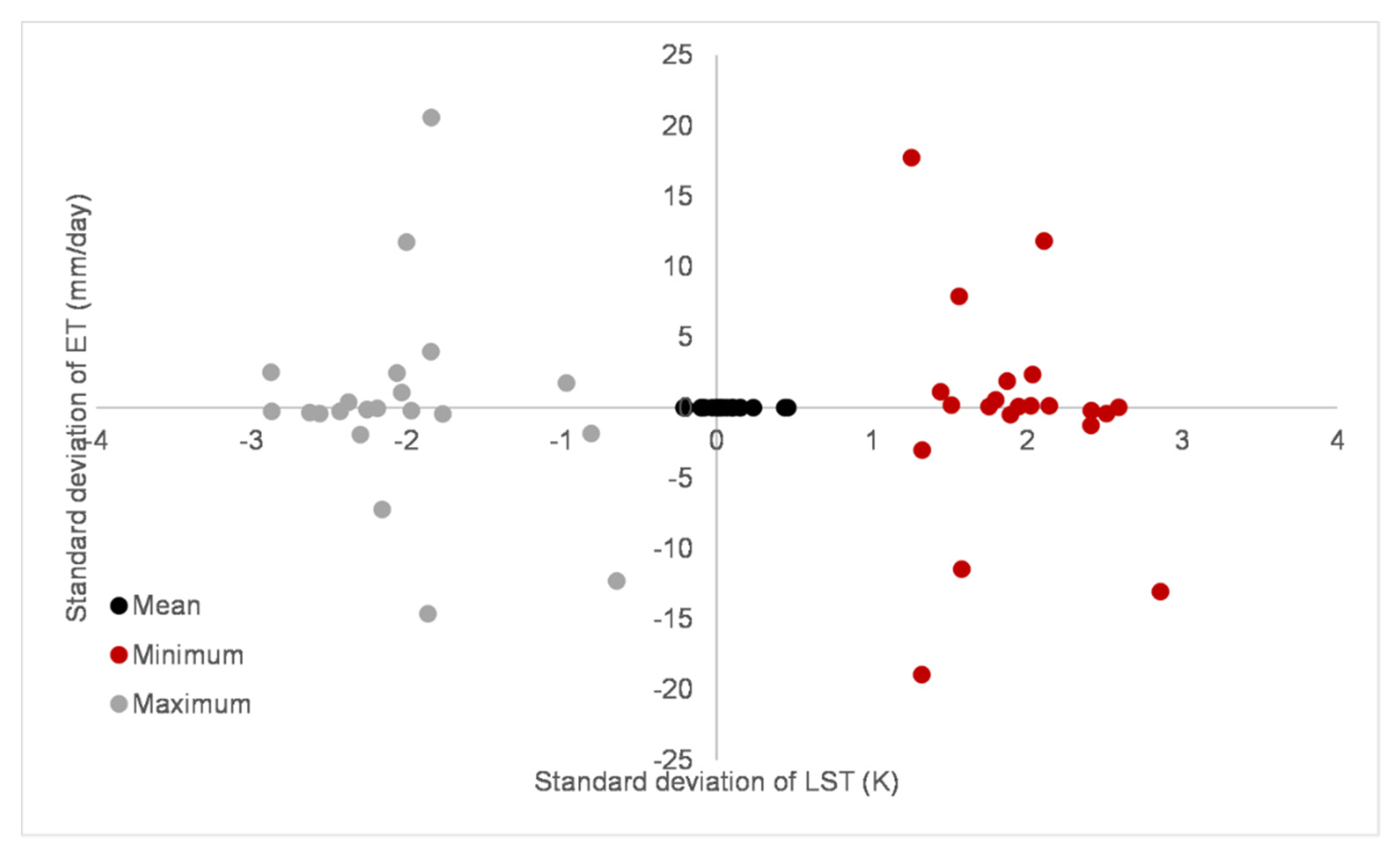
3.2. Heterogeneity of the Study Area

The performance of applying remote sensing data to ET calculation is related to the concept of spatial variability of the landscape, especially in selecting the spatial resolution of the sensor. Low spatial resolution sensors, in more heterogeneous landscapes, generate less reliable ET results since intra-pixel spatial heterogeneity is lost due to radiometric signal integration [9,49,50,51,52]. Besides the importance of the choice of the satellite sensor, Gibson et al. [9] studied the variability of ET influenced by heterogeneity of landcover, analyzing topography, fractional vegetation cover, NDVI and albedo, the authors found uncertainties which are translated to the estimation of actual evapotranspiration. In Brazil, a study performed at Caatinga has proved that the land use, substantially affects the components of the net radiation that depend on the type and state of the land surface cover, such as reflected shortwave radiation and emitted longwave radiation [53].

In order to understand the heterogeneity and seasonality of the study area in our site, Figure 3 shows an example of NDVI distribution for each season, in which it can be seen the differences between summer/spring and winter/autumn. The most homogeneity in the area occurred in winter season. This behavior can be responsible for the high seasonal variability of evapotranspiration, with higher values during the spring-summer period when compared to autumn-winter observed in Pampa biome by [7].

The ET variability by the landcover heterogeneity are shown in Figure 4 where three different land uses were selected and the averages ET of each one was calculated. We compared the differences between Native Grassland, Exposed Soil and Forest with the daily ET average for each day. The daily ET seasonality in summer is twice as high as in winter, which was already expected because of the high temperature variability at different times of the year, characteristic of the study region.

Gibson et al. [9] reported that in addition to the direct effect of landscape heterogeneity and spatial resolution of input data on remote sensing variables, landscape heterogeneity can also indirectly affect spatial modelling efforts, including the energy fluxes. The ET variability between Forest and Grassland were lower than expected, demonstrating the importance of native grasslands in the Pampa biome regarding to the processes of the hydrological cycle, since it covers 63% of Rio Grande do Sul, with the greatest differences occurring randomly during the warmer and colder seasons.

It is important to emphasize that the native grassland area of this study has an adequate livestock management controlled by the Federal University of Santa Maria. Studies conducted in field areas with high exploitation management have obtained greater differences in water balance results when compared with forested areas [54].

The seasonality of the Pampa biome, Figure 5, was explained by preview studies which discussed the strong seasonality of ET in the region, with the highest rates of ET in the summer and spring period [7,43,55,56]. In warmer periods there is usually higher energy availability, rapid vegetation development, higher biomass accumulation, which also indicates a higher ET [43]. During the colder seasons (autumn and winter), the small growth in the Pampa grasslands all of the biomass production is consumed by cattle, which is typical in this biome [57]. In this sense, an adequate land use management is essential for the maintenance of native species in the region that also favor livestock farming and are dependent on water cycle.

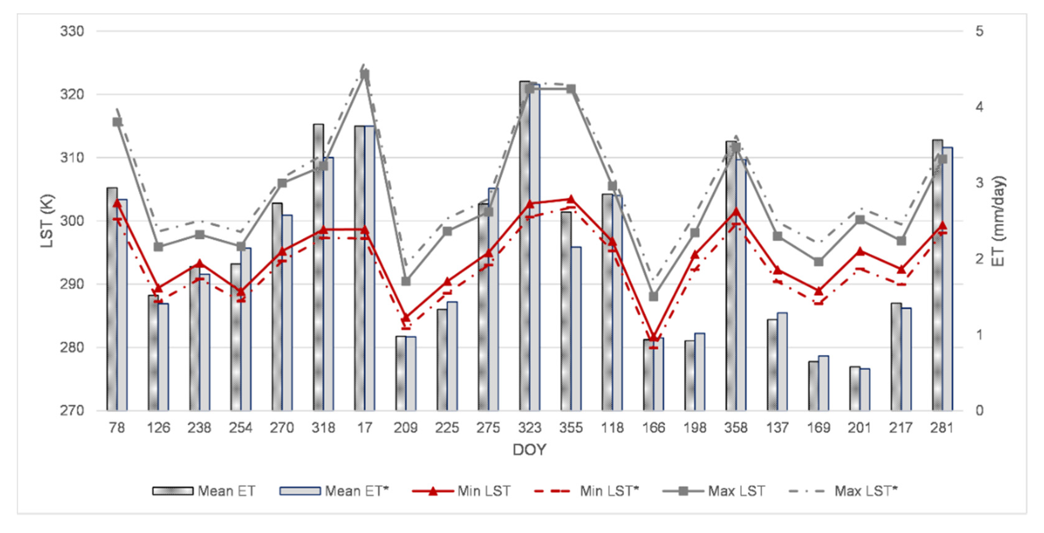
3.3. The Ts Influence on S-SEBI Model

The errors or uncertainties in analysis of remote sensing and GIS products can be associated with several sources. According to Gibson et al. most of them are: (1) associated with the specific remote sensing data obtained; (2) introduced with the processing and analysis of image and field data; (3) associated with positional aspects (including image resolution); and (4) associated with the specific model. In this regard, the uncertainties in the derivation of ET for this study were identified in the relationship between Ts and albedo for the S-SEBI model performance for the selected days between 2015–2019. In addition, there is an influence of Rn on LE results, discussed in Section 3.1, and consequently on ET.

Table 5. Comparison between energy fluxes with and without noise in a native grassland (in situ data): Min–Max is minimum and maximum values, r² is the coefficient of determination (–), MSD is the mean standard deviation (W/m²), RMSE refers to the Root Mean Square Error (W/m²); and Bias is the tendency of the model (W/m²).

Variable	Min–Max	Min–Max (*)	r2	MSD	RMSE	Bias
LE (W/m2)	52.88–431.22	74.51–408.95	0.98	±21.13	19.36	11.48
Rn (W/m2)	142.44–536.05	140.33–533.95	1	±0.14	1.98	1.97
G (W/m2)	7.41–86.07	7.55–86.48	1	±19.28	0.27	−0.24

* with noise on Land Surface Temperature.

shows the comparison of energy partitioning between S-SEBI results with and without noise in the Ts in a native grassland. The minimum and maximum values in the fluxes have changed when the noise was applied, LE flux has the highest shift, the difference decreases 11%, while in the other flows the changes did not cause significant differences, less than 1%. This is because LE is based on the correct selection of hot and cold pixels which are highly dependent on Ts values, this dependence is strongly studied by several authors [6,8,58,59].

This difference in LE estimations are demonstrated by statistical analyses with a RMSE 19.36 W/m² and Bias 11.48 (W/m²), this result is lower than other models reported in the literature, which are more dependent on meteorological data. Su (2002) [60] found out a sensitivity of SEBS model around 40 W/m² when the various terms are assumed independent of each other.

The differences in the other fluxes when the noise in Ts is applied are not significant, with extremely low errors and variances as RMSE (1.98 and 0.27) and Bias (1.97 and 0.24) to Rn and G, respectively.

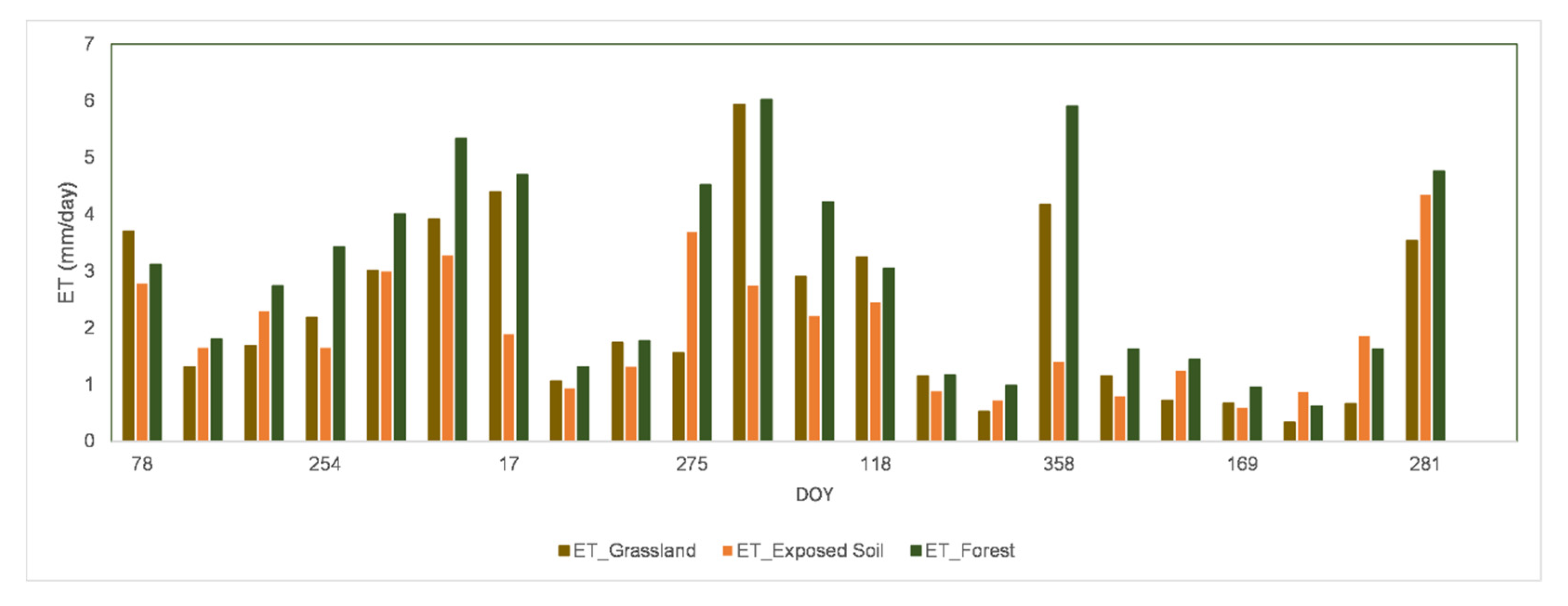
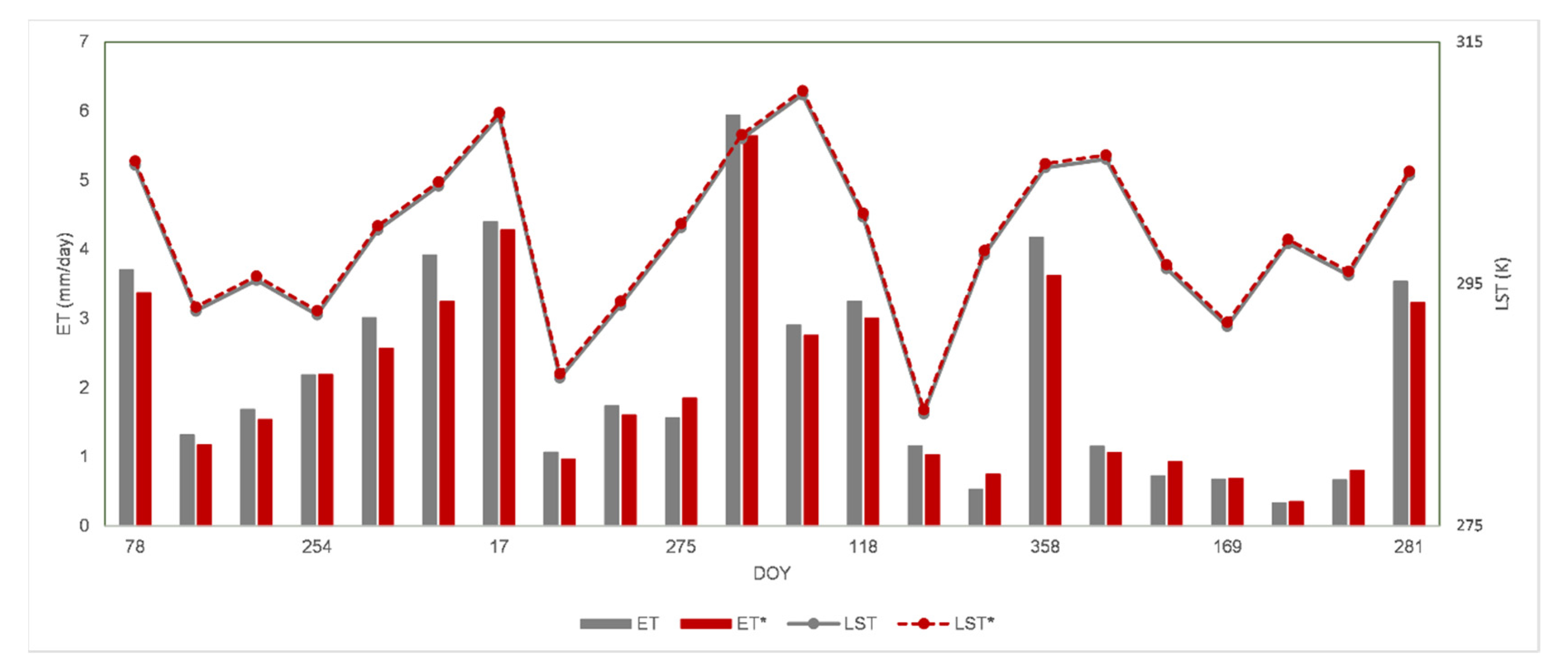
3.4. The Ts Influence on Daily Evapotranspiration

The natural grassland daily ET mean error between both analyses (with and without noise in Ts) is 0.18 mm/day for the whole period studied, those variance to each day at tower flux point are shown in Figure 6. Gibson et al. [9] have analyzed the SEBS model, and conclude that daily ET differences by up to 0.7 mm/day when modifying Ts and air temperature. We concluded that the gaussian variation of Ts (between −2 K and 2 K) leads to a small variation of ET, it does not exceed 0.5 mm/day in grasslands. Abid et al. [10] are in accordance with this result finding similar value (0.5 mm/day) when comparing de uncertainties of SEBS model in Northern Tunisia.

Figure 7 shows the resulting changes in Mean, Maximum and Minimum ET against Ts considering all scene. The gaussian noise applied is a random noise, so it is probable that the maximum Ts pixel value of an image is not the same as in the noisy image, therefore the maximum and minimum are modified in more than a 2 K noise applied. The differences in maximum and minimum Ts caused by the noise applied affect ET values, but the mean ET are less affected by these differences on mean Ts of the scenes. The biggest differences on mean ET occurred on summer in 2015 with 0.44 mm/day, but the minimum and maximus ET have generated the biggest changes, these values occurred in forest or in exposed soil areas. The changes in maximum and minimum ET were expected because S-SEBI model has difficulty in reaching extremely high values [18,47].

When there are uncertainties in estimates of Ts, the errors in the estimates of the daily ET multiply for the entire study area, as shown in Figure 8, the maximum and minimum values of Ts are responsible for the variation in the ET estimated, even with the same mean Ts for the images. We can see that Ts have biggest range during summer seasons and on winter seasons de maximum and minimum Ts are closer, but that differences do not influence the changes in daily ET. These results demonstrate the importance of Ts’ accuracy in the selection of the driest and wettest pixels, thus being the greatest challenge in applying S-SEBI to estimate ET season-independent even though the seasonal variability of ET.

4. Discussion

Many studies have been carried out in the Pampa biome with the objective of understanding how different agricultural management affects this ecosystem [15,22,57,61,62,63,64], but few studies are aimed how the energy balance is affected by these activities [7,43,56,65,66]. It is important to emphasize that the native grassland of Pampa biome is important not only for the preservation of the biodiversity of endemic species in the region, but also for the sustainable development of rural families [19,22,67,68]. In this sense this work brings a new variable to this equation, that the native grasslands with adequate management are so important for the energy balance as the forests found in the region.

According to Fontana et al. [49] the weather station affects and modifies the accumulation of forage in the natural grasslands of the Pampa biome, which is typical of the subtropical climate prevailing in the region. In this sense, winter is the critical season for livestock production, which corroborates with the results of this work that demonstrates the decrease of evapotranspiration in winter indicating less forage production.

Some complexities associated with the derivation of ET and discussed by Gibson et al. [9] imply that potential errors will be introduced at various stages of ET derivation, including the heterogeneity of the area and meteorological data. From the energy point of view, evapotranspiration is dependent on latent heat flux. It is in this context that the models (such as SEBAL, S-SEBI, SEBS, SEBTA, SAFER) that calculate ET by remote sensing are based. In this study we used S-SEBI which depends mainly on the relationship between albedo and Ts.

This is the first study developed in the Pampa biome that seeks to understand the influence of the Ts on energy balance fluxes and daily ET, some studies have been developed with the objective of understanding the environmental and atmospheric influences on remote sensing evapotranspiration models, but none of them evaluate the S-SEBI [9,10,60].

The accuracies of most Ts retrieval algorithms are between 1 and 2 K [26,36,69]. In this sense, this work demonstrates that for the S-SEBI model, although these differences in temperature affect the choice of hot and cold pixels of images and to estimate LE, the possible errors generated by retrieve Ts and emissivity do not affect the results in daily evapotranspiration so significantly (0.5 mm/day). Also, the method used in the conversion of LE to daily ET, explained in the Section 2.3, contributes to reduce the errors of the one-time estimate, because it considers the global radiation behavior throughout the day [18].

5. Conclusions

In order to estimate daily evapotranspiration (ET) using S-SEBI model and remote sensing technologies from Landsat 8, a sensitivity study of output ET was performed with a Gaussian noise variability in LST images. The S-SEBI model estimates ET from the relationship between LST and albedo. This study allowed to understand the influence that the uncertainties in LST estimation may have on the ET.

The accuracy of the Rn validation has aggregated some uncertainties in the model, (more than 100 W/m²), these errors might be related to the use of reanalysis data. Therefore, an evaluation regarding the sensibility of this data on energy balance models is indicated for future works.

The lower ET variability between forest and native grassland can demonstrate the importance of native grasslands in the Pampa biome regarding to the processes of the hydrological cycle, since it covers 63% of Rio Grande do Sul. It also indicates that in Pampa biome the native grassland is not only important to the biodiversity conservation but also to the environment process. Future studies may provide more conclusions about the influences of different native grasslands managements.

The gaussian variation of LST (between −2 K and 2 K) do not influence the average of the variable and leads to a small variation of ET, it does not exceed 0.5 mm/day in grasslands, with mean error between both analyses (with and without noise in LST) around 0.18 mm/day for the whole period studied.

We concluded that the S-SEBI is less dependent on LST estimation than other models reported in the literature, such as the SEBS largely studied [9,10]. However, the importance of LST’s accuracy in the selection of driest and wettest pixels was proved.

References

1. Olioso, A.; Chauki, H.; Courault, D.; Wigneron, J.-P. Estimation of Evapotranspiration and Photosynthesis by Assimilation of Remote Sensing Data into SVAT Models. Remote Sens. Environ. 1999, 68, 341–356. [Google Scholar] [CrossRef]
2. Ehsan Bhuiyan, M.A.; Nikolopoulos, E.I.; Anagnostou, E.N.; Polcher, J.; Albergel, C.; Dutra, E.; Fink, G.; Martínez-de la Torre, A.; Munier, S. Assessment of precipitation error propagation in multi-model global water resource reanalysis. Hydrol. Earth Syst. Sci. 2019, 23, 1973–1994. [Google Scholar] [CrossRef] [Green Version]
3. Courault, D.; Seguin, B.; Olioso, A. Review on estimation of evapotranspiration from remote sensing data: From empirical to numerical modeling approaches. Irrig. Drain. Syst. 2005, 19, 223–249. [Google Scholar] [CrossRef]
4. Priestley, C.H.B.; Taylor, R.J. On the assessment of surfaceheat flux and evaporation using large-scale parameters. Mon Weather Rev 1972, 100, 81–92. [Google Scholar]
5. Wang, T.; Tang, R.; Li, Z.L.; Jiang, Y.; Liu, M.; Niu, L. An improved spatio-temporal adaptive Data fusion algorithm for evapotranspiration mapping. Remote Sens. 2019, 11, 761. [Google Scholar] [CrossRef] [Green Version]
6. Cristóbal, J.; Jiménez-Muñoz, J.C.; Prakash, A.; Mattar, C.; Skoković, D.; Sobrino, J.A. An improved single-channel method to retrieve land surface temperature from the landsat-8 thermal band. Remote Sens. 2018, 10, 431. [Google Scholar] [CrossRef] [Green Version]
7. Rubert, G.C.; Roberti, D.R.; Pereira, L.S.; Quadros, F.L.; Campos Velho, H.F.D.; Leal de Moraes, O.L. Evapotranspiration of the Brazilian Pampa biome: Seasonality and influential factors. Water 2018, 10, 1864. [Google Scholar] [CrossRef] [Green Version]
8. Sobrino, J.A.; Gómez, M.; Jiménez-Muñoz, J.C.; Olioso, A.; Chehbouni, G. A simple algorithm to estimate evapotranspiration from DAIS data: Application to the DAISEX campaigns. J. Hydrol. 2005, 315, 117–125. [Google Scholar] [CrossRef] [Green Version]
9. Gibson, L.A.; Münch, Z.; Engelbrecht, J. Particular uncertainties encountered in using a pre-packaged SEBS model to derive evapotranspiration in a heterogeneous study area in South Africa. Hydrol. Earth Syst. Sci. 2011, 15, 295–310. [Google Scholar] [CrossRef] [Green Version]
10. Abid, N.; Mannaerts, C.; Bargaoui, Z. Sensitivity of actual evapotranspiration estimation using the sebs model to variation of input parameters (LST, DSSF, aerodynamics parameters, LAI, FVC). Int. Arch. Photogramm. Remote Sens. Spat. Inf. Sci. ISPRS Arch. 2019, 42, 1193–1200. [Google Scholar] [CrossRef] [Green Version]
11. Oki, T.; Kanae, S. Global Hydrological Cycles and World Water Resources. Science 2006, 313, 1068–1072. [Google Scholar] [CrossRef] [Green Version]
12. Cheng, J.; Kustas, W. Using Very High Resolution Thermal Infrared Imagery for More Accurate Determination of the Impact of Land Cover Differences on Evapotranspiration in an Irrigated Agricultural Area. Remote Sens. 2019, 11, 613. [Google Scholar] [CrossRef] [Green Version]
13. Liu, S.; Su, H.; Zhang, R.; Tian, J.; Chen, S.; Wang, W.; Yang, L.; Liang, H. Based on the Gaussian fitting method to derive daily evapotranspiration from remotely sensed instantaneous evapotranspiration. Adv. Meteorol. 2019, 2019. [Google Scholar] [CrossRef]
14. Liou, Y.A.; Kar, S.K. Evapotranspiration estimation with remote sensing and various surface energy balance algorithms-a review. Energies 2014, 7, 2821–2849. [Google Scholar] [CrossRef] [Green Version]
15. Souza, V.D.A.; Roberti, D.R.; Ruhoff, A.L.; Zimmer, T.; Adamatti, D.S.; Gonçalves, L.G.G.D.; Diaz, M.B.; Alves, R.D.C.M.; Moraes, O.L.L.D. Evaluation of MOD16 Algorithm over Irrigated Rice Paddy Using Flux Tower Measurements in Southern Brazil. Water 2019, 11, 1911. [Google Scholar] [CrossRef] [Green Version]
16. Roerink, G.J.; Su, Z.; Menenti, M. S-SEBI: A simple remote sensing algorithm to estimate the surface energy balance. Phys. Chem. Earth, Part B Hydrol. Ocean. Atmos. 2000, 25, 147–157. [Google Scholar] [CrossRef]
17. Gómez, M.; Olioso, A.; Sobrino, J.A.; Jacob, F. Retrieval of evapotranspiration over the Alpilles/ReSeDA experimental site using airborne POLDER sensor and a thermal camera. Remote Sens. Environ. 2005, 96, 399–408. [Google Scholar] [CrossRef]
18. Sobrino, J.A.; Gómez, M.; Jiménez-Muñoz, J.C.; Olioso, A. Application of a simple algorithm to estimate daily evapotranspiration from NOAA-AVHRR images for the Iberian Peninsula. Remote Sens. Environ. 2007, 110, 139–148. [Google Scholar] [CrossRef]
19. Vargas, L.P.; da Costa Vargas, A.F.; Silveira, V.C.P. Ecosystem services and production systems of family cattle farms: An analysis of animal production in Pampa Biome. Semin. Ciências Agrárias 2020, 41, 661–676. [Google Scholar]
20. Rocha, J.M. As Raízes da Crise da Metade Sul: Estudo da formação econômica do Rio Grande do Sul.; UNIPAMPA: Jaguarão-RS, Brazil, 2011. [Google Scholar]
21. Pylro, V.S.; Morais, D.K.; Roesch, L.F.W. Microbiome studies need local leaders. Nature 2015, 528, 39. [Google Scholar] [CrossRef]
22. Overbeck, G.E.; Müller, S.C.; Pillar, V.D.; Pfadenhauer, J. Floristic composition, environmental variation and species distribution patterns in burned grassland in southern Brazil. Brazilian J. Biol. 2006, 66, 1073–1090. [Google Scholar] [CrossRef] [PubMed]
23. Oliveira, L.B.; Soares, E.M.; Jochims, F.; Tiecher, T.; Marques, A.R.; Kuinchtner, B.C.; Rheinheimer, D.S.; De Quadros, F.L.F. Long-Term Effects of Phosphorus on Dynamics of an Overseeded Natural Grassland in Brazil. Rangel. Ecol. Manag. 2015, 68, 445–452. [Google Scholar] [CrossRef]
24. Confortin, A.C.C.; Quadros, F.L.F.; Santos, A.B.; Seibert, L.; Severo, P.O.; Ribeiro, B.S.R. Leaf tissue fluxes of Pampa biome native grasses submitted to two grazing intervals. Grass Forage Sci. 2017, 72, 654–662. [Google Scholar] [CrossRef]
25. Sauer, T.J.; Horton, R. Soil Heat Flux. In Agronomy Monographs; Hatfield, J.L., Baker, J.M., Eds.; American Society of Agronomy, Crop Science Society of America, and Soil Science Society of America: Madison, WI, USA, 2015; pp. 131–154. ISBN 9780891182689. [Google Scholar]
26. Jimenez-Munoz, J.C.; Sobrino, J.A.; Skokovic, D.; Mattar, C.; Cristobal, J. Land surface temperature retrieval methods from landsat-8 thermal infrared sensor data. IEEE Geosci. Remote Sens. Lett. 2014, 11, 1840–1843. [Google Scholar] [CrossRef]
27. Kilic, A.; Allen, R.; Trezza, R.; Ratcliffe, I.; Kamble, B.; Robison, C.; Ozturk, D. Sensitivity of evapotranspiration retrievals from the METRIC processing algorithm to improved radiometric resolution of Landsat 8 thermal data and to calibration bias in Landsat 7 and 8 surface temperature. Remote Sens. Environ. 2016, 185, 198–209. [Google Scholar] [CrossRef] [Green Version]
28. Rouse, J.W.; Haas, R.H.; Schell, J.A.; Deering, D.W. Monitoring Vegetation Systems in the Great Plains with ERTS. In Proceedings of the Third ERTS-1 Symposium; NASA: Washington, DC, USA, 1973; pp. 309–317. [Google Scholar]
29. Ke, Y.; Im, J.; Park, S.; Gong, H. Downscaling of MODIS One kilometer evapotranspiration using Landsat-8 data and machine learning approaches. Remote Sens. 2016, 8, 215. [Google Scholar] [CrossRef] [Green Version]
30. Sobrino, J.A.; Li, Z.L.; Stoll, M.P.; Becker, F. Multi-channel and multi-angle algorithms for estimating sea and land surface temperature with ATSR data. Int. J. Remote Sens. 1996, 17, 2089–2114. [Google Scholar] [CrossRef]
31. Buck, A.L. New Equations for Computing Vapor Pressure and Enhancement Factor. J. Appl. Meteorol. 1981, 20, 1527–1532. [Google Scholar] [CrossRef] [Green Version]
32. Sobrino, J.A.; Jiménez-Muñoz, J.C.; Sòria, G.; Romaguera, M.; Guanter, L.; Moreno, J.; Plaza, A.; Martínez, P. Land surface emissivity retrieval from different VNIR and TIR sensors. IEEE Trans. Geosci. Remote Sens. 2008, 46, 316–327. [Google Scholar] [CrossRef]
33. Bastiaanssen, W.G.M. SEBAL-based sensible and latent heat fluxes in the irrigated Gediz Basin, Turkey. J. Hydrol. 2000, 229, 87–100. [Google Scholar] [CrossRef]
34. Skokovic, D.; Sobrino, J.A.; Jimenez-Munoz, J.C. Vicarious Calibration of the Landsat 7 Thermal Infrared Band and LST Algorithm Validation of the ETM+ Instrument Using Three Global Atmospheric Profiles. IEEE Trans. Geosci. Remote Sens. 2017, 55, 1804–1811. [Google Scholar] [CrossRef]
35. Sobrino, J.A.; Skoković, D. Permanent Stations for Calibration/Validation of Thermal Sensors over Spain. Data 2016, 1, 10. [Google Scholar] [CrossRef]
36. Kafer, P.S.; Rolim, S.B.A.; Iglesias, M.L.; da Rocha, N.S.; Diaz, L.R. Land Surface Temperature Retrieval by LANDSAT 8 Thermal Band: Applications of Laboratory and Field Measurements. IEEE J. Sel. Top. Appl. Earth Obs. Remote Sens. 2019, 12, 2332–2341. [Google Scholar] [CrossRef]
37. Aubinet, M.; Vesala, T.; Papale, D. Eddy Covariance—A Practical Guide to Measurement and Data Analysis; Springer: Berlin/Heidelberg, Germany, 2012. [Google Scholar]
38. Kljun, N.; Calanca, P.; Rotach, M.W.; Schmid, H.P. A simple parameterisation for flux footprint predictions. Bound. Layer Meteorol. 2004, 112, 503–523. [Google Scholar] [CrossRef]
39. Twine, T.E.; Kustas, W.P.; Norman, J.M.; Cook, D.R.; Houser, P.R.; Meyers, T.P.; Prueger, J.H.; Starks, P.J.; Wesely, M.L. Correcting eddy-covariance flux underestimates over a grassland. Agric. For. Meteorol. 2000, 103, 279–300. [Google Scholar] [CrossRef] [Green Version]
40. de Oliveira, G.; Brunsell, N.; Moraes, E.; Bertani, G.; dos Santos, T.; Shimabukuro, Y.; Aragão, L. Use of MODIS Sensor Images Combined with Reanalysis Products to Retrieve Net Radiation in Amazonia. Sensors 2016, 16, 956. [Google Scholar] [CrossRef] [Green Version]
41. Mayer, D.G.; Butler, D.G. Statistical validation. Ecol. Model. 1993, 68, 21–32. [Google Scholar] [CrossRef]
42. Olioso, A.; Chauki, H.; Courault, D.; Wigneron, J. Available online: https://www.sciencedirect.com/science/article/abs/pii/S0034425798001217 (accessed on 23 September 2020).
43. Schirmbeck, J.; Fontana, D.C.; Roberti, D.R. Evaluation of OSEB and SEBAL models for energy balance of a crop area in a humid subtropical climate. Bragantia 2018, 77, 609–621. [Google Scholar] [CrossRef] [Green Version]
44. Silva Oliveira, B.; Caria Moraes, E.; Carrasco-Benavides, M.; Bertani, G.; Augusto Verola Mataveli, G. Improved Albedo Estimates Implemented in the METRIC Model for Modeling Energy Balance Fluxes and Evapotranspiration over Agricultural and Natural Areas in the Brazilian Cerrado. Remote Sens. 2018, 10, 1181. [Google Scholar] [CrossRef] [Green Version]
45. Romio, L.C.; Roberti, D.R.; Buligon, L.; Zimmer, T.; Degrazia, G.A. A Numerical Model to Estimate the Soil Thermal Conductivity Using Field Experimental Data. Appl. Sci. 2019, 9, 4799. [Google Scholar] [CrossRef] [Green Version]
46. Zimmer, T.; Buligon, L.; de Arruda Souza, V.; Romio, L.C.; Roberti, D.R. Influence of clearness index and soil moisture in the soil thermal dynamic in natural pasture in the Brazilian Pampa biome. Geoderma 2020, 378, 114582. [Google Scholar] [CrossRef]
47. Gomis-Cebolla, J.; Jimenez, J.C.; Sobrino, J.A.; Corbari, C.; Mancini, M. Intercomparison of remote-sensing based evapotranspiration algorithms over amazonian forests. Int. J. Appl. Earth Obs. Geoinf. 2019, 80, 280–294. [Google Scholar] [CrossRef]
48. Zahira, S.; Abderrahmane, H.; Mederbal, K.; Frederic, D. Mapping Latent Heat Flux in the Western Forest Covered Regions of Algeria Using Remote Sensing Data and a Spatialized Model. Remote Sens. 2009, 1, 795–817. [Google Scholar] [CrossRef] [Green Version]
49. KUSTAS, W.P.; NORMAN, J.M. Use of remote sensing for evapotranspiration monitoring over land surfaces. Hydrol. Sci. J. 1996, 41, 495–516. [Google Scholar] [CrossRef]
50. Garrigues, S.; Allard, D.; Baret, F.; Weiss, M. Influence of landscape spatial heterogeneity on the non-linear estimation of leaf area index from moderate spatial resolution remote sensing data. Remote Sens. Environ. 2006, 105, 286–298. [Google Scholar] [CrossRef]
51. McCabe, M.F.; Wood, E.F. Scale influences on the remote estimation of evapotranspiration using multiple satellite sensors. Remote Sens. Environ. 2006, 105, 271–285. [Google Scholar] [CrossRef]
52. Chen, Y.; Xia, J.; Liang, S.; Feng, J.; Fisher, J.B.; Li, X.; Li, X.; Liu, S.; Ma, Z.; Miyata, A.; et al. Comparison of satellite-based evapotranspiration models over terrestrial ecosystems in China. Remote Sens. Environ. 2014, 140, 279–293. [Google Scholar] [CrossRef]
53. Ferreira, T.R.; Da Silva, B.B.; Moura, M.S.B.D.; Verhoef, A.; Nóbrega, R.L.B. The use of remote sensing for reliable estimation of net radiation and its components: A case study for contrasting land covers in an agricultural hotspot of the Brazilian semiarid region. Agric. For. Meteorol. 2020, 291, 108052. [Google Scholar] [CrossRef]
54. Cruz, J.C.; Valente, M.L.; Baggiotto, C.; Baumhardt, E. Qualitative characteristics of water resulting from the introduction of Eucalyptus silviculture in Pampa biome, RS. RBRH 2016, 21, 636–645. [Google Scholar] [CrossRef]
55. Rubert, G.C.D.; Roberti, D.R.; Diaz, M.B.; Moraes, O.L.L. de Estimativa Da Evapotranspiração Em Área De Pastagem Em Santa Maria—Rs. Ciência e Nat. 2016, 38, 300. [Google Scholar] [CrossRef]
56. Fontana, D.C.; Junges, A.H.; Bremm, C.; Schaparini, L.P.; Mengue, V.P.; Wagner, A.P.L.; Carvalho, P. NDVI and meteorological data as indicators of the Pampa biome natural grasslands growth. Bragantia 2018, 77, 404–414. [Google Scholar] [CrossRef] [Green Version]
57. Scottá, F.C.; da Fonseca, E.L. Multiscale trend analysis for pampa grasslands using ground data and vegetation sensor imagery. Sensors 2015, 15, 17666–17692. [Google Scholar] [CrossRef] [PubMed] [Green Version]
58. Mattar, C.; Franch, B.; Sobrino, J.A.; Corbari, C.; Jiménez-Muñoz, J.C.; Olivera-Guerra, L.; Skokovic, D.; Sória, G.; Oltra-Carriò, R.; Julien, Y.; et al. Impacts of the broadband albedo on actual evapotranspiration estimated by S-SEBI model over an agricultural area. Remote Sens. Environ. 2014, 147, 23–42. [Google Scholar] [CrossRef]
59. Bastiaanssen, W.G.M.; Pelgrum, H.; Wang, J.; Ma, Y.; Moreno, J.F.; Roerink, G.J.; Van Der Wal, T. A remote sensing surface energy balance algorithm for land (SEBAL): 2. Validation. J. Hydrol. 1998, 212–213, 213–229. [Google Scholar] [CrossRef]
60. Su, Z. The Surface Energy Balance System (SEBS) for estimation of turbulent heat fluxes. Hydrol. Earth Syst. Sci. 2002, 6, 85–100. [Google Scholar] [CrossRef]
61. Beatriz, A.; Carvalho, P.; Ozorio, C.P. Avaliação Sobre Os Banhados Do Rio Grande Do Sul, Brasil. Rev. Ciências Ambient. 2007, 1, 83–95. [Google Scholar]
62. Santos, T.; Trevisan, R. Eucaliptos versus bioma Pampa: Compreendendo as diferenças entre lavouras de arbóreas e o campo nativo. In: TEIXEIRA FILHO, A. (Org.). Lavouras de Destruição A (im)posição do consenso 2009, 299–332. [Google Scholar]
63. OVERBECK, G.E.; MÜLLER, S.C.; Fidelis, A.T.; PFADENHAUER, J.; PILLAR, V.; BLANCO, C.C.; BOLDRINI, I.I.; BOTH, R.; FORNECK, E.D. Brazil’s neglected biome: The South Brazilian Campos. Perspect. Plant Ecol. Evol. Syst. 2007, 9, 101–116. [Google Scholar] [CrossRef]
64. Käfer, P.S.; da Rocha, N.S.; Diaz, L.R.; Kaiser, E.A.; Santos, D.C.; Veeck, G.P.; Robérti, D.R.; Rolim, S.B.A.; Oliveira, G.G. Artificial neural networks model based on remote sensing to retrieve evapotranspiration over the Brazilian Pampa. J. Appl. Remote Sens. 2020, 14. [Google Scholar] [CrossRef]
65. Diaz, M.B.; Roberti, D.R.; Carneiro, J.V.; de Arruda Souza, V.; de Moraes, O.L.L. Dynamics of the superficial fluxes over a flooded rice paddy in southern Brazil. Agric. For. Meteorol. 2019, 276–277, 107650. [Google Scholar] [CrossRef]
66. Monteiro, P.F.C.; Fontana, D.C.; dos Santos, T.V.; Roberti, D.R. Estimativa dos componentes do balanço de energia e da evapotranspiração para áreas de cultivo de soja no sul do brasil utilizando imagens do sensor TM landsat 5. Bragantia 2014, 73, 72–80. [Google Scholar] [CrossRef]
67. OVERBECK, G.E.; Podgaiski, L.R.; MÜLLER, S.C. Biodiversidade dos campos. In Campos do Sul.; PILLAR, V., Lange, O., Eds.; Rede Campos Sulios: Porto Alegre, Brazil, 2015; pp. 43–50. [Google Scholar]
68. Rocha, J.M. Silvio Cezar Arend Desenvolvimento E Sustentabilidade Na Agricultura Da Metade Sul Do Rs: Parâmetros. In Proceedings of the VIII Seminário Internacional sobre Desenvolvimento Regional; Unisc, PPG Desenvolvimento Regional: Santa Cruz do Sul, Brazil, 2017. [Google Scholar]
69. Käfer, P.S.; Rolim, S.B.A.; Heinz, L.V.O.; Iglesias, M.L.; da Rocha, N.S.; Diaz, L.R. Assessment of single-channel algorithms for land surface temperature retrieval at two southern Brazil sites. J. Appl. Remote Sens. 2020, 14, 1. [Google Scholar] [CrossRef]
Figure 1. American Pampa Biome and Tower Flux location.
Atmosphere 11 01059 g001
Figure 2. Energy balance components estimated with S-SEBI against in-situ data. The black line represents the 1:1 relation.
Atmosphere 11 01059 g002
Figure 3. NDVI distribution for the study area for a summer season scene (DOY 17); autumn season scene (DOY 126); winter season scene (DOY 254) and a spring season scene (DOY 323).
Atmosphere 11 01059 g003
Figure 4. Daily evapotranspiration (mm/day) for different land surface uses in Pampa biome.
Atmosphere 11 01059 g004
Figure 5. Spatial Daily evapotranspiration (mm/day) for different seasons in Pampa biome.
Atmosphere 11 01059 g005
Figure 6. Grassland (in situ) daily evapotranspiration (mm/day) and Land Surface Temperature (K) with and without noise (*).
Atmosphere 11 01059 g006
Figure 7. Changes of daily evapotranspiration (ET mm/day) against the changes of land surface temperature (Ts) input by gaussian variation of 2 K.
Atmosphere 11 01059 g007
Figure 8. Minimum and Maximum Land Surface Temperature (Kelvin) and Mean daily evapotranspiration (mm/day) of the entire study area. * without noise on Land Surface Temperature.
Atmosphere 11 01059 g008