Investigating the Impacts of Urbanization on PM2.5 Pollution in the Yangtze River Delta of China: A Spatial Panel Data Approach

 ,
,  , ,
, ,  ,
,
Abstract
1. Introduction
2. Data and Methods
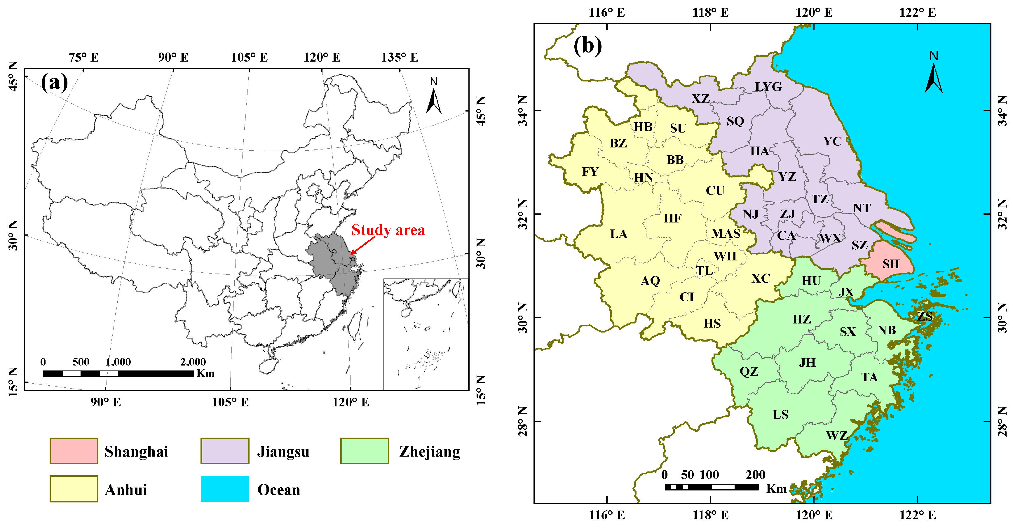
2.1. Study Area
2.2. Data
2.2.1. PM2.5 Data
2.2.2. Urbanization and Other Factors
2.2.3. Variables Selection
2.3. Methods
2.3.1. Trend Analysis
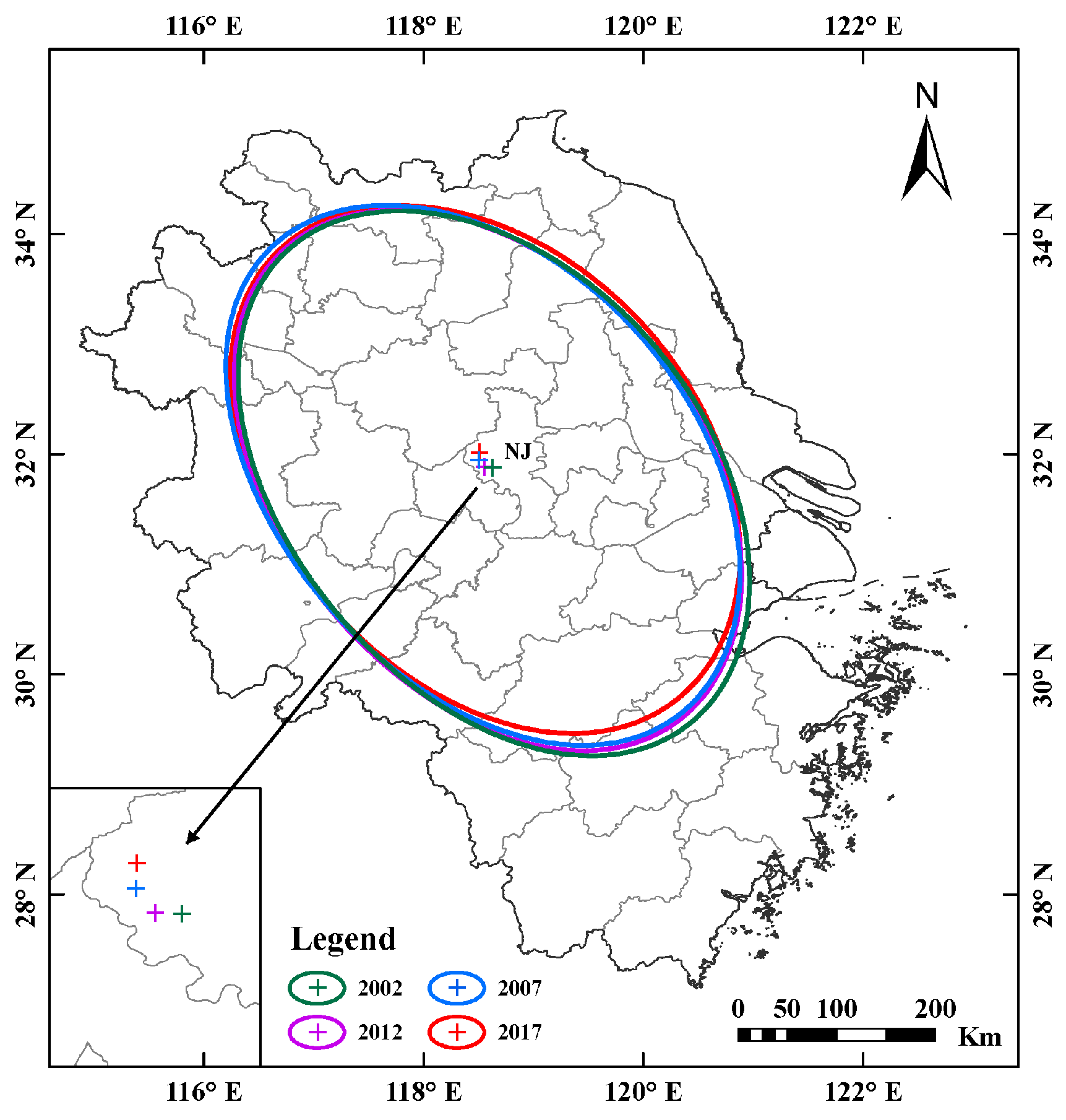
2.3.2. Standard Deviation Ellipse Analysis
2.3.3. Spatial Autocorrelation Analysis
2.3.4. Spatial Regression Analysis
3. Results
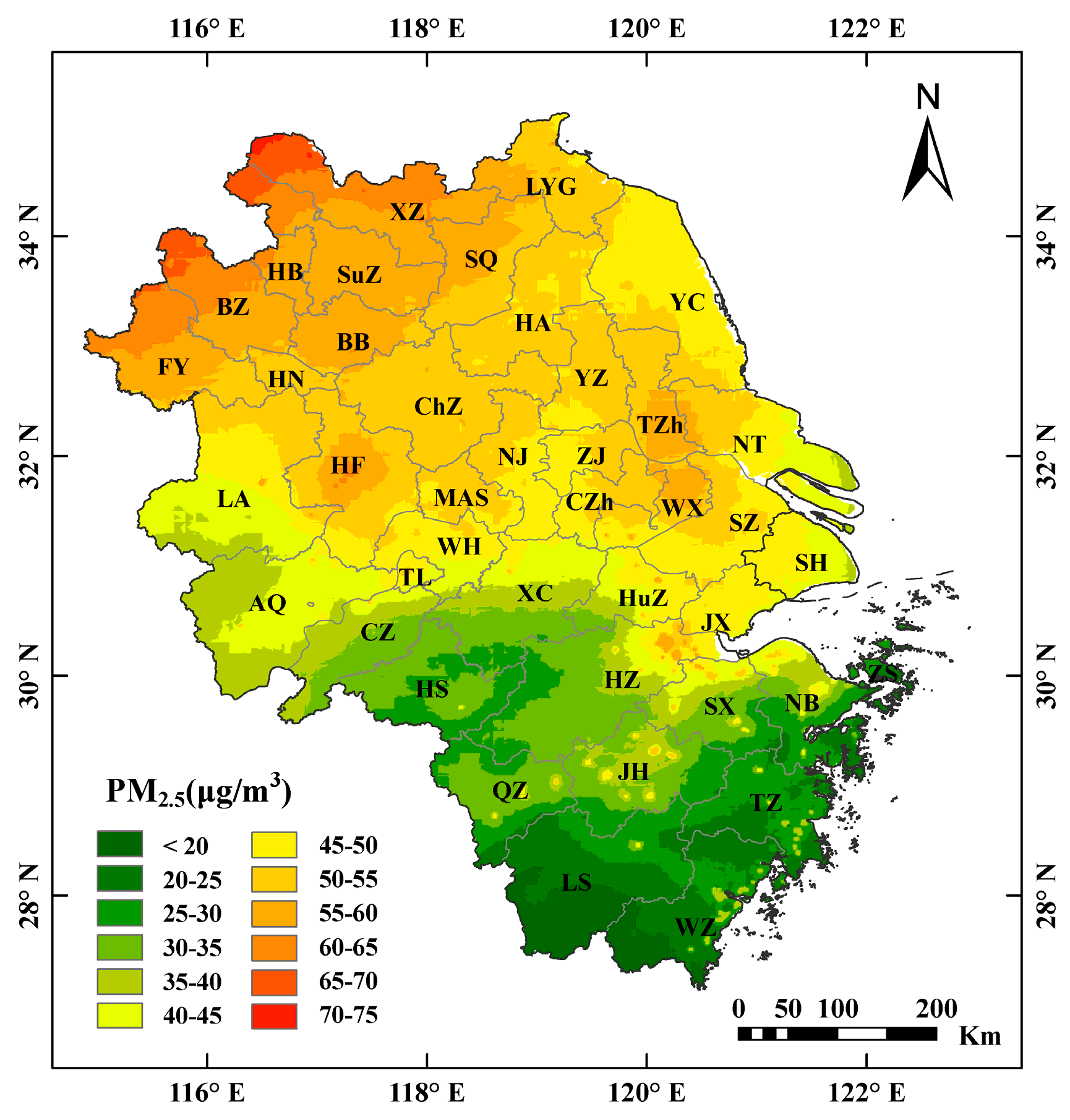
3.1. Spatial Pattern of PM2.5 Pollution
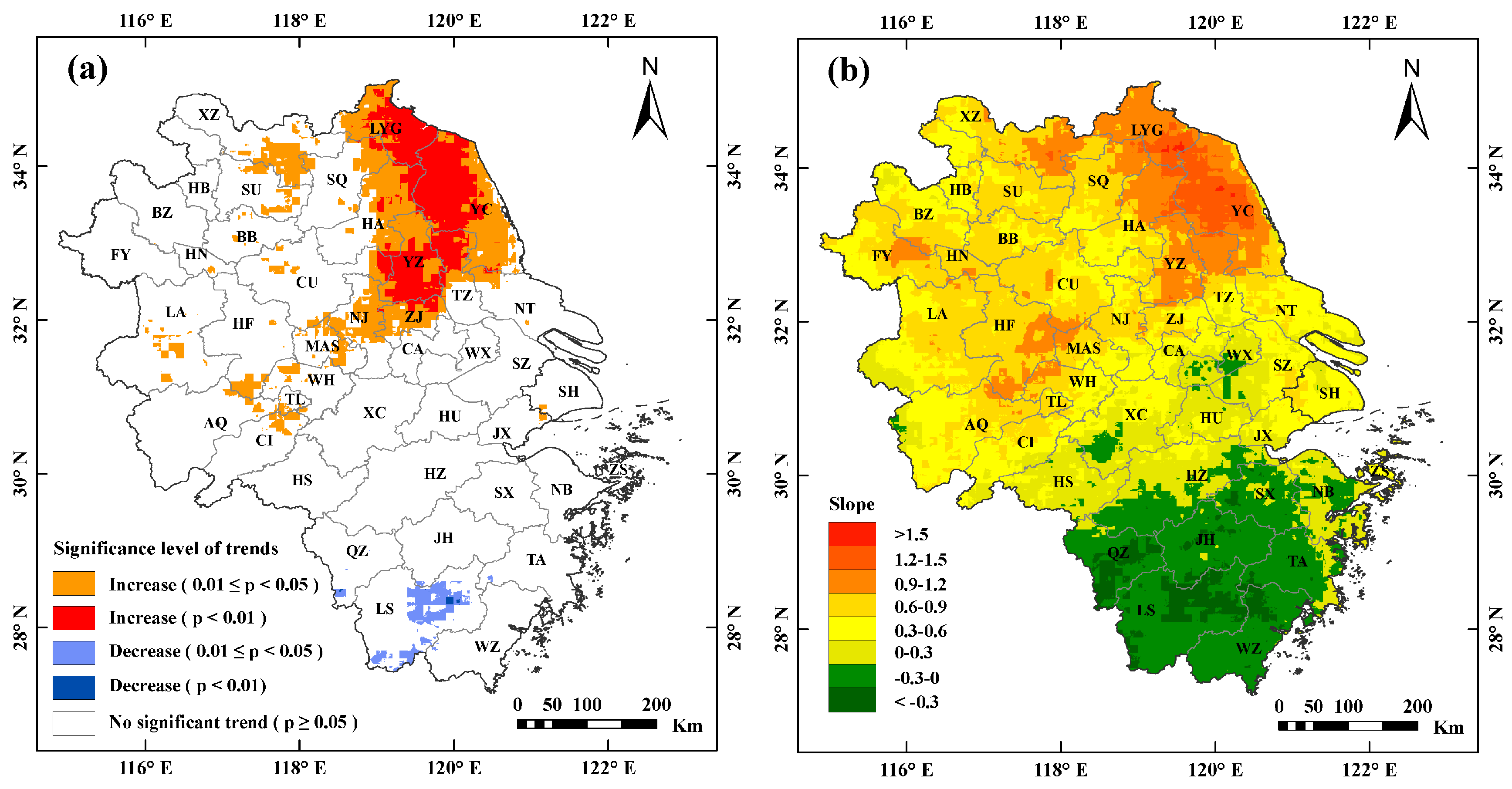
3.2. Trends of PM2.5 Concentrations
3.3. Spatial Autocorrelation Analysis
3.4. Spatial Panel Regression Analysis
3.4.1. Results of Model Tests
3.4.2. Estimation Results
4. Discussion
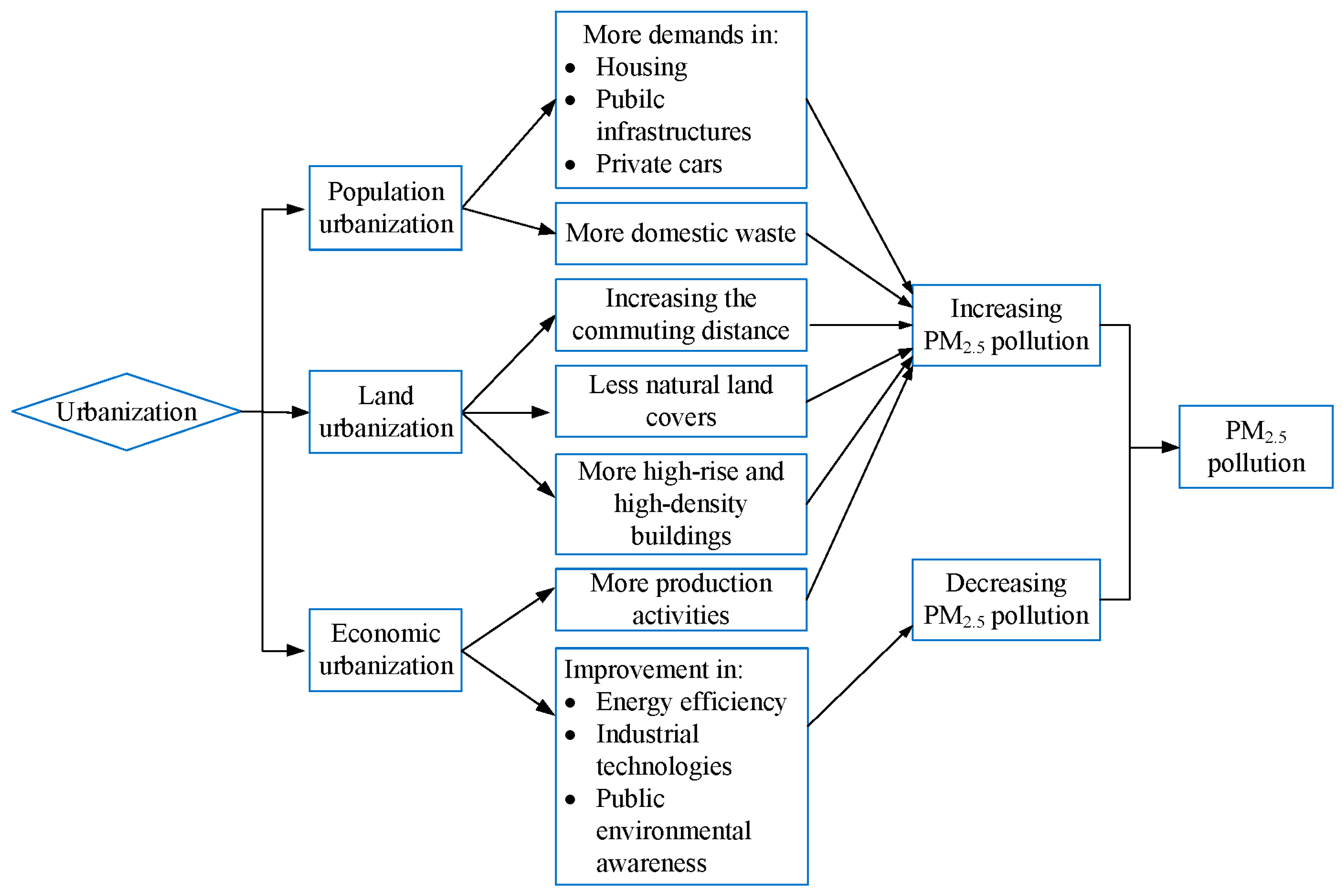
4.1. The Impacts of Urbanization on PM2.5 Pollution
4.2. The Impacts of other Factors on PM2.5 Concentrations
4.3. Policy Implications
4.4. Limitation
5. Conclusions
- Distinct variation in the spatial pattern of the PM2.5 concentrations was identified in the YRD. Approximately 83.57% of the YRD had mean PM2.5 concentrations higher than 35 ug/m3 (WHO Interim Target 1). The pollution was more severe in the north than in the south part of the YRD.
- The significant and largest increasing trends in PM2.5 pollution was noticed in Lianyungang and Yancheng cities. However, the regional median center of the PM2.5 pollution was located in the Nanjing city and was gradually shifting to the northwest during the research period.
- The positive spatial autocorrelation and spillover effect of PM2.5 pollution were verified by the global Moran’s I values and the SDM model, respectively, thus suggesting that the prevention and control of air pollution should rely on inter-regional cooperation.
- Population urbanization, land urbanization, secondary industry and NDVI exerted significant impacts on PM2.5 pollution. Population urbanization had the largest positive total effect, followed by land urbanization and secondary industry, while NDVI showed a negative total effect. No significant effect was detected for economic urbanization.
Supplementary Materials
Author Contributions
Funding
Conflicts of Interest
References
- Hallquist, M.; Wenger, J.C.; Baltensperger, U.; Rudich, Y.; Simpson, D.; Claeys, M.; Dommen, J.; Donahue, N.M.; George, C.; Goldstein, A.H.; et al. The formation, properties and impact of secondary organic aerosol: Current and emerging issues. Atmos. Chem. Phys. 2009, 9, 5155–5236. [Google Scholar] [CrossRef]
- Zhang, R.; Jing, J.; Tao, J.; Hsu, S.C.; Wang, G.; Cao, J.; Lee, C.S.L.; Zhu, L.; Chen, Z.; Zhao, Y.; et al. Chemical characterization and source apportionment of PM2.5 in Beijing: Seasonal perspective. Atmos. Chem. Phys. 2013, 13, 7053–7074. [Google Scholar] [CrossRef]
- Dominici, F.; Peng, R.D.; Bell, M.L.; Pham, L.; McDermott, A.; Zeger, S.L.; Samet, J.M. Fine particulate air pollution and hospital admission for cardiovascular and respiratory diseases. JAMA 2006, 295, 1127. [Google Scholar] [CrossRef] [PubMed]
- Fann, N.; Lamson, A.D.; Anenberg, S.C.; Wesson, K.; Risley, D.; Hubbell, B.J. Estimating the national public health burden associated with exposure to ambient PM2.5 and ozone. Risk Anal. 2012, 32, 81–95. [Google Scholar] [CrossRef]
- Hoek, G.; Krishnan, R.M.; Beelen, R.; Peters, A.; Ostro, B.; Brunekreef, B.; Kaufman, J.D. Long-term air pollution exposure and cardio- respiratory mortality: A review. Environ. Health 2013, 12, 43. [Google Scholar] [CrossRef]
- Aklesso, M.; Kumar, K.R.; Bu, L.; Boiyo, R. Analysis of spatial-temporal heterogeneity in remotely sensed aerosol properties observed during 2005–2015 over three countries along the Gulf of Guinea Coast in Southern West Africa. Atmos. Environ. 2018, 182, 313–324. [Google Scholar] [CrossRef]
- Pui, D.Y.H.; Chen, S.-C.; Zuo, Z. PM2.5 in China: Measurements, sources, visibility and health effects, and mitigation. Particuology 2014, 13, 1–26. [Google Scholar] [CrossRef]
- Zhang, Y.; Shuai, C.; Bian, J.; Chen, X.; Wu, Y.; Shen, L. Socioeconomic factors of PM2.5 concentrations in 152 Chinese cities: Decomposition analysis using LMDI. J. Clean. Prod. 2019, 218, 96–107. [Google Scholar] [CrossRef]
- Ministry of Environmental Protection of the People’s Republic of China. Report on the state of the environment in China, 2013. Available online: http://english.mee.gov.cn/Resources/Reports/soe/Report/201706/P020170614504782926467.pdf (accessed on 1 April 2020).
- Liang, L.; Wang, Z.; Li, J. The effect of urbanization on environmental pollution in rapidly developing urban agglomerations. J. Clean. Prod. 2019, 237, 117649. [Google Scholar] [CrossRef]
- Zhou, C.; Wang, S.; Wang, J. Examining the influences of urbanization on carbon dioxide emissions in the Yangtze River Delta, China: Kuznets curve relationship. Sci. Total Environ. 2019, 675, 472–482. [Google Scholar] [CrossRef]
- Zhu, W.; Wang, M.; Zhang, B. The effects of urbanization on PM2.5 concentrations in China’s Yangtze River Economic Belt: New evidence from spatial econometric analysis. J. Clean. Prod. 2019, 239, 118065. [Google Scholar] [CrossRef]
- Civerolo, K.; Hogrefe, C.; Lynn, B.; Rosenthal, J.; Ku, J.Y.; Solecki, W.; Cox, J.; Small, C.; Rosenzweig, C.; Goldberg, R.; et al. Estimating the effects of increased urbanization on surface meteorology and ozone concentrations in the New York City metropolitan region. Atmos. Environ. 2007, 41, 1803–1818. [Google Scholar] [CrossRef]
- De Ridder, K.; Lefebre, F.; Adriaensen, S.; Arnold, U.; Beckroege, W.; Bronner, C.; Damsgaard, O.; Dostal, I.; Dufek, J.; Hirsch, J.; et al. Simulating the impact of urban sprawl on air quality and population exposure in the German Ruhr area. Part II: Development and evaluation of an urban growth scenario. Atmos. Environ. 2008, 42, 7070–7077. [Google Scholar] [CrossRef]
- Martins, H. Urban compaction or dispersion? An air quality modelling study. Atmos. Environ. 2012, 54, 60–72. [Google Scholar] [CrossRef]
- Han, L.; Zhou, W.; Li, W.; Qian, Y. Urbanization strategy and environmental changes: An insight with relationship between population change and fine particulate pollution. Sci. Total Environ. 2018, 642, 789–799. [Google Scholar] [CrossRef] [PubMed]
- Baklanov, A.; Molina, L.T.; Gauss, M. Megacities, air quality and climate. Atmos. Environ. 2016, 126, 235–249. [Google Scholar] [CrossRef]
- Lu, D.; Xu, J.; Yue, W.; Mao, W.; Yang, D.; Wang, J. Response of PM2.5 pollution to land use in China. J. Clean. Prod. 2020, 244, 118741. [Google Scholar] [CrossRef]
- Manes, F.; Marando, F.; Capotorti, G.; Blasi, C.; Salvatori, E.; Fusaro, L.; Ciancarella, L.; Mircea, M.; Marchetti, M.; Chirici, G.; et al. Regulating Ecosystem Services of forests in ten Italian Metropolitan Cities: Air quality improvement by PM10 and O3 removal. Ecol. Indic. 2016, 67, 425–440. [Google Scholar] [CrossRef]
- Janhäll, S. Review on urban vegetation and particle air pollution - Deposition and dispersion. Atmos. Environ. 2015, 105, 130–137. [Google Scholar] [CrossRef]
- Feng, Y.; Wang, X. Effects of urban sprawl on haze pollution in China based on dynamic spatial Durbin model during 2003–2016. J. Clean. Prod. 2020, 242, 118368. [Google Scholar] [CrossRef]
- Du, Y.; Sun, T.; Peng, J.; Fang, K.; Liu, Y.; Yang, Y.; Wang, Y. Direct and spillover effects of urbanization on PM2.5 concentrations in China’s top three urban agglomerations. J. Clean. Prod. 2018, 190, 72–83. [Google Scholar] [CrossRef]
- Sohag, K.; Begum, R.A.; Abdullah, S.M.S.; Jaafar, M. Dynamics of energy use, technological innovation, economic growth and trade openness in Malaysia. Energy 2015, 90, 1497–1507. [Google Scholar] [CrossRef]
- Fan, X.; Xu, Y. Convergence on the haze pollution: City-level evidence from China. Atmos. Pollut. Res. 2020, 11, 141–152. [Google Scholar] [CrossRef]
- Dong, F.; Zhang, S.; Long, R.; Zhang, X.; Sun, Z. Determinants of haze pollution: An analysis from the perspective of spatiotemporal heterogeneity. J. Clean. Prod. 2019, 222, 768–783. [Google Scholar] [CrossRef]
- Wu, J.; Zhang, P.; Yi, H.; Qin, Z. What causes haze pollution? An empirical study of PM2.5 concentrations in Chinese cities. Sustainability 2016, 8, 132. [Google Scholar] [CrossRef]
- Lee, C. Impacts of urban form on air quality: Emissions on the road and concentrations in the US metropolitan areas. J. Environ. Manag. 2019, 246, 192–202. [Google Scholar] [CrossRef]
- Jiménez-Parra, B.; Alonso-Martínez, D.; Godos-Díez, J.L. The influence of corporate social responsibility on air pollution: Analysis of environmental regulation and eco-innovation effects. Corp. Soc. Responsib. Environ. Manag. 2018, 25, 1363–1375. [Google Scholar] [CrossRef]
- Han, L.; Zhou, W.; Li, W.; Li, L. Impact of urbanization level on urban air quality: A case of fine particles (PM2.5) in Chinese cities. Environ. Pollut. 2014, 194, 163–170. [Google Scholar] [CrossRef]
- Botlaguduru, V.S.V.; Kommalapati, R.R. Meteorological detrending of long-term (2003-2017) ozone and precursor concentrations at three sites in the Houston Ship Channel Region. J. Air Waste Manag. Assoc. 2020, 70, 93–107. [Google Scholar] [CrossRef]
- Alcántara, V.; Padilla, E.; Piaggio, M. Nitrogen oxide emissions and productive structure in Spain: An input–output perspective. J. Clean. Prod. 2017, 141, 420–428. [Google Scholar] [CrossRef]
- Giannakis, E.; Kushta, J.; Giannadaki, D.; Georgiou, G.K.; Bruggeman, A.; Lelieveld, J. Exploring the economy-wide effects of agriculture on air quality and health: Evidence from Europe. Sci. Total Environ. 2019, 663, 889–900. [Google Scholar] [CrossRef] [PubMed]
- Román, R.; Cansino, J.M.; Rueda-Cantuche, J.M. A multi-regional input-output analysis of ozone precursor emissions embodied in Spanish international trade. J. Clean. Prod. 2016, 137, 1382–1392. [Google Scholar] [CrossRef]
- Del Sarto, S.; Marino, M.F.; Ranalli, M.G.; Salvati, N. Using finite mixtures of M-quantile regression models to handle unobserved heterogeneity in assessing the effect of meteorology and traffic on air quality. Stoch. Environ. Res. Risk Assess. 2019, 33, 1345–1359. [Google Scholar] [CrossRef]
- Otero, N.; Sillmann, J.; Schnell, J.L.; Rust, H.W.; Butler, T. Synoptic and meteorological drivers of extreme ozone concentrations over Europe. Environ. Res. Lett. 2016, 11, 024005. [Google Scholar] [CrossRef]
- Schuch, D.; de Freitas, E.D.; Espinosa, S.I.; Martins, L.D.; Carvalho, V.S.B.; Ramin, B.F.; Silva, J.S.; Martins, J.A.; de Fatima Andrade, M. A two decades study on ozone variability and trend over the main urban areas of the São Paulo state, Brazil. Environ. Sci. Pollut. Res. 2019, 26, 31699–31716. [Google Scholar] [CrossRef]
- Hajiloo, F.; Hamzeh, S.; Gheysari, M. Impact assessment of meteorological and environmental parameters on PM2.5 concentrations using remote sensing data and GWR analysis (case study of Tehran). Environ. Sci. Pollut. Res. 2019, 26, 24331–24345. [Google Scholar] [CrossRef]
- Alahmadi, S.; Al-Ahmadi, K.; Almeshari, M. Spatial variation in the association between NO2 concentrations and shipping emissions in the Red Sea. Sci. Total Environ. 2019, 676, 131–143. [Google Scholar] [CrossRef]
- Shi, Y.; Ren, C.; Lau, K.K.-L.; Ng, E. Investigating the influence of urban land use and landscape pattern on PM2.5 spatial variation using mobile monitoring and WUDAPT. Landsc. Urban Plan. 2019, 189, 15–26. [Google Scholar] [CrossRef]
- Cheng, L.; Li, L.; Chen, L.; Hu, S.; Yuan, L.; Liu, Y.; Cui, Y.; Zhang, T. Spatiotemporal variability and influencing factors of aerosol optical depth over the Pan Yangtze River Delta during the 2014–2017 period. Int. J. Environ. Res. Public Health 2019, 16, 3522. [Google Scholar] [CrossRef]
- Liu, H.; Fang, C.; Zhang, X.; Wang, Z.; Bao, C.; Li, F. The effect of natural and anthropogenic factors on haze pollution in Chinese cities: A spatial econometrics approach. J. Clean. Prod. 2017, 165, 323–333. [Google Scholar] [CrossRef]
- Balado-Naves, R.; Baños-Pino, J.F.; Mayor, M. Do countries influence neighbouring pollution? A spatial analysis of the EKC for CO2 emissions. Energy Policy 2018, 123, 266–279. [Google Scholar] [CrossRef]
- Maddison, D. Modelling sulphur emissions in Europe: A spatial econometric approach. Oxf. Econ. Pap. 2007, 59, 726–743. [Google Scholar] [CrossRef]
- Marbuah, G.; Amuakwa-Mensah, F. Spatial analysis of emissions in Sweden. Energy Econ. 2017, 68, 383–394. [Google Scholar] [CrossRef]
- Du, Y.; Wan, Q.; Liu, H.; Liu, H.; Kapsar, K.; Peng, J. How does urbanization influence PM2.5 concentrations? Perspective of spillover effect of multi-dimensional urbanization impact. J. Clean. Prod. 2019, 220, 974–983. [Google Scholar] [CrossRef]
- Elhorst, J.P. Spatial Econometrics: From Cross-Sectional Data to Spatial Panels, 1st ed.; Springer: Berlin/Heidelberg, Germany, 2014; pp. 1–3. ISBN 978-3-642-40339-2. [Google Scholar]
- Ding, Y.; Zhang, M.; Chen, S.; Wang, W.; Nie, R. The environmental Kuznets curve for PM2.5 pollution in Beijing-Tianjin-Hebei region of China: A spatial panel data approach. J. Clean. Prod. 2019, 220, 984–994. [Google Scholar] [CrossRef]
- Yun, G.; He, Y.; Jiang, Y.; Dou, P.; Dai, S. PM2.5 spatiotemporal evolution and drivers in the Yangtze river delta between 2005 and 2015. Atmosphere (Basel) 2019, 10, 55. [Google Scholar] [CrossRef]
- Yang, D.; Chen, Y.; Miao, C.; Liu, D. Spatiotemporal variation of PM2.5 concentrations and its relationship to urbanization in the Yangtze river delta region, China. Atmos. Pollut. Res. 2019, 11, 491–498. [Google Scholar] [CrossRef]
- Lu, D.; Mao, W.; Yang, D.; Zhao, J.; Xu, J. Effects of land use and landscape pattern on PM2.5 in Yangtze River Delta, China. Atmos. Pollut. Res. 2018, 9, 705–713. [Google Scholar] [CrossRef]
- RESDC (Data Center for Resources and Environmental Sciences, Chinese Academy of Sciences). Available online: http://www.resdc.cn (accessed on 22 October 2019).
- Zhang, X.; Chen, L.; Yuan, R. Effect of natural and anthropic factors on the spatiotemporal pattern of haze pollution control of China. J. Clean. Prod. 2020, 251, 119531. [Google Scholar] [CrossRef]
- Atmospheric Composition Analysis Group. Available online: http://fizz.phys.dal.ca/~atmos/martin/?page_id=140 (accessed on 18 November 2019).
- Van Donkelaar, A.; Martin, R.V.; Brauer, M.; Hsu, N.C.; Kahn, R.A.; Levy, R.C.; Lyapustin, A.; Sayer, A.M.; Winker, D.M. Global estimates of fine particulate matter using a combined geophysical-statistical method with information from satellites, models, and monitors. Environ. Sci. Technol. 2016, 50, 3762–3772. [Google Scholar] [CrossRef]
- Van Donkelaar, A.; Martin, R.V.; Li, C.; Burnett, R.T. Regional estimates of chemical composition of fine particulate matter using a combined geoscience-statistical method with information from satellites, models, and monitors. Environ. Sci. Technol. 2019, 53, 2595–2611. [Google Scholar] [CrossRef] [PubMed]
- Van Donkelaar, A.; Martin, R.V.; Brauer, M.; Boys, B.L. Use of satellite observations for long-term exposure assessment of global concentrations of fine particulate matter. Environ. Health Perspect. 2015, 123, 135–143. [Google Scholar] [CrossRef] [PubMed]
- Li, J.; Han, X.; Jin, M.; Zhang, X.; Wang, S. Globally analysing spatiotemporal trends of anthropogenic PM2.5 concentration and population’s PM2.5 exposure from 1998 to 2016. Environ. Int. 2019, 128, 46–62. [Google Scholar] [CrossRef] [PubMed]
- National Bureau of Statistics of China. China City Statistical Yearbook (2003-2018). Available online: https://data.cnki.net/yearbook/Single/N2020050229 (accessed on 1 March 2020). (In Chinese).
- Huang, J.; Liu, C.; Chen, S.; Huang, X.; Hao, Y. The convergence characteristics of China’s carbon intensity: Evidence from a dynamic spatial panel approach. Sci. Total Environ. 2019, 668, 685–695. [Google Scholar] [CrossRef]
- China Meteorological Data Service Center. Available online: http://data.cma.cn/en (accessed on 20 November 2019).
- Li, L.; Zhou, X.; Chen, L.; Chen, L.; Zhang, Y.; Liu, Y. Estimating urban vegetation biomass from Sentinel-2A image data. Forests 2020, 11, 125. [Google Scholar] [CrossRef]
- Kang, Y.; Zhao, T.; Yang, Y. Environmental Kuznets curve for CO2 emissions in China: A spatial panel data approach. Ecol. Indic. 2016, 63, 231–239. [Google Scholar] [CrossRef]
- Kendall, M.G. Rank Correlation Methods, 4th ed.; Charles Griffin: London, UK, 1975; ISBN 978 0852641996. [Google Scholar]
- Bari, M.A.; Kindzierski, W.B. Eight-year (2007–2014) trends in ambient fine particulate matter (PM2.5) and its chemical components in the Capital Region of Alberta, Canada. Environ. Int. 2016, 91, 122–132. [Google Scholar] [CrossRef]
- Chatterjee, S.; Khan, A.; Akbari, H.; Wang, Y. Monotonic trends in spatio-temporal distribution and concentration of monsoon precipitation (1901–2002), West Bengal, India. Atmos. Res. 2016, 182, 54–75. [Google Scholar] [CrossRef]
- Mann, H.B. Nonparametric tests against trend. Econometrica 1945, 13, 245–259. [Google Scholar] [CrossRef]
- Zhao, N.; Jiao, Y.; Ma, T.; Zhao, M.; Fan, Z.; Yin, X.; Liu, Y.; Yue, T. Estimating the effect of urbanization on extreme climate events in the Beijing-Tianjin-Hebei region, China. Sci. Total Environ. 2019, 688, 1005–1015. [Google Scholar] [CrossRef]
- Sen, P.K. Estimates of the regression coefficient based on Kendall’s tau. J. Am. Stat. Assoc. 1968, 63, 1379–1389. [Google Scholar] [CrossRef]
- Ribeiro, L.; Kretschmer, N.; Nascimento, J.; Buxo, A.; Rötting, T.; Soto, G.; Señoret, M.; Oyarzún, J.; Maturana, H.; Oyarzún, R. Evaluating piezometric trends using the Mann-Kendall test on the alluvial aquifers of the Elqui River basin, Chile. Hydrol. Sci. J. 2015, 60, 1840–1852. [Google Scholar] [CrossRef]
- Nyelele, C.; Kroll, C.N. The equity of urban forest ecosystem services and benefits in the Bronx, NY. Urban For. Urban Green. 2020, 53, 126723. [Google Scholar] [CrossRef]
- Lorelei de Jesus, A.; Thompson, H.; Knibbs, L.D.; Kowalski, M.; Cyrys, J.; Niemi, J.V.; Kousa, A.; Timonen, H.; Luoma, K.; Petäjä, T.; et al. Long-term trends in PM2.5 mass and particle number concentrations in urban air: The impacts of mitigation measures and extreme events due to changing climates. Environ. Pollut. 2020, 263, 114500. [Google Scholar] [CrossRef]
- Peng, J.; Chen, S.; Lü, H.; Liu, Y.; Wu, J. Spatiotemporal patterns of remotely sensed PM2.5 concentration in China from 1999 to 2011. Remote Sens. Environ. 2016, 174, 109–121. [Google Scholar] [CrossRef]
- Shi, Y.; Matsunaga, T.; Yamaguchi, Y.; Zhao, A.; Li, Z.; Gu, X. Long-term trends and spatial patterns of PM2.5-induced premature mortality in South and Southeast Asia from 1999 to 2014. Sci. Total Environ. 2018, 631–632, 1504–1514. [Google Scholar] [CrossRef]
- Li, H.; Li, L.; Chen, L.; Zhou, X.; Cui, Y.; Liu, Y.; Liu, W. Mapping and characterizing spatiotemporal dynamics of impervious surfaces using Landsat images: A case study of Xuzhou, East China from 1995 to 2018. Sustainability 2019, 11, 1224. [Google Scholar] [CrossRef]
- Rahman, M.; Yang, R.; Di, L. Clustering Indian Ocean tropical cyclone tracks by the standard deviational ellipse. Climate 2018, 6, 39. [Google Scholar] [CrossRef]
- Cui, Y.; Li, L.; Chen, L.; Zhang, Y.; Cheng, L.; Zhou, X.; Yang, X. Land-use carbon emissions estimation for the Yangtze River Delta Urban Agglomeration using 1994–2016 Landsat image data. Remote Sens. 2018, 10, 1334. [Google Scholar] [CrossRef]
- Getis, A. A history of the concept of spatial autocorrelation: A geographer’s perspective. Geogr. Anal. 2008, 40, 297–309. [Google Scholar] [CrossRef]
- Li, H.; Calder, C.A.; Cressie, N. Beyond Moran’s I: Testing for spatial dependence based on the spatial autoregressive model. Geogr. Anal. 2007, 39, 357–375. [Google Scholar] [CrossRef]
- Moran, P.A.P. Notes on continuous stochastic phenomena. Biometrika 1950, 37, 17–23. [Google Scholar] [CrossRef] [PubMed]
- Glass, A.J.; Kenjegalieva, K.; Sickles, R.C. A spatial autoregressive stochastic frontier model for panel data with asymmetric efficiency spillovers. J. Econom. 2016, 190, 289–300. [Google Scholar] [CrossRef]
- Li, M.; Li, C.; Zhang, M. Exploring the spatial spillover effects of industrialization and urbanization factors on pollutants emissions in China’s Huang-Huai-Hai region. J. Clean. Prod. 2018, 195, 154–162. [Google Scholar] [CrossRef]
- Elhorst, J.P. Matlab software for spatial panels. Int. Reg. Sci. Rev. 2014, 37, 389–405. [Google Scholar] [CrossRef]
- Bottasso, A.; Conti, M.; Ferrari, C.; Tei, A. Ports and regional development: A spatial analysis on a panel of European regions. Transp. Res. Part A Policy Pract. 2014, 65, 44–55. [Google Scholar] [CrossRef]
- Elhorst, J.P. Applied spatial econometrics: Raising the bar. Spat. Econ. Anal. 2010, 5, 9–28. [Google Scholar] [CrossRef]
- LeSage, J.; Pace, R.K. Introduction to Spatial Econometrics; CRC Press Taylor & Francis Group: Boca Raton, FL, USA, 2009; pp. 45–75. ISBN 9781420064254. [Google Scholar]
- Elhorst, J.P. Dynamic spatial panels: models, methods, and inferences. J. Geogr. Syst. 2012, 14, 5–28. [Google Scholar] [CrossRef]
- Wooldridge, J.M. Econometric Analysis of Cross Section and Panel Data, 2nd ed.; The MIT Press: London, UK, 2010; pp. 281–334. ISBN 9780262232586. [Google Scholar]
- Wang, X.; Tian, G.; Yang, D.; Zhang, W.; Lu, D.; Liu, Z. Responses of PM2.5 pollution to urbanization in China. Energy Policy 2018, 123, 602–610. [Google Scholar] [CrossRef]
- Stone, B. Urban sprawl and air quality in large US cities. J. Environ. Manag. 2008, 86, 688–698. [Google Scholar] [CrossRef]
- Weng, Q.; Yang, S. Urban air pollution patterns, land use, and thermal landscape: An examination of the linkage using GIS. Environ. Monit. Assess. 2006, 117, 463–489. [Google Scholar] [CrossRef] [PubMed]
- Li, X.; Song, H.; Zhai, S.; Lu, S.; Kong, Y.; Xia, H.; Zhao, H. Particulate matter pollution in Chinese cities: Areal-temporal variations and their relationships with meteorological conditions (2015–2017). Environ. Pollut. 2019, 246, 11–18. [Google Scholar] [CrossRef] [PubMed]
- Chen, C.; Sun, Y.; Lan, Q.; Jiang, F. Impacts of industrial agglomeration on pollution and ecological efficiency-A spatial econometric analysis based on a big panel dataset of China’s 259 cities. J. Clean. Prod. 2020, 258, 120721. [Google Scholar] [CrossRef]
- Guo, L.; Luo, J.; Yuan, M.; Huang, Y.; Shen, H.; Li, T. The influence of urban planning factors on PM2.5 pollution exposure and implications: A case study in China based on remote sensing, LBS, and GIS data. Sci. Total Environ. 2019, 659, 1585–1596. [Google Scholar] [CrossRef] [PubMed]


| Variable | Abbreviation | Definition | Unit |
|---|---|---|---|
| PM2.5 | PM | Concentration of PM2.5 | μg/m3 |
| Ratio of urban population | PU | Urban population/total population | % |
| Ratio of urban built-up area | LU | Urban built-up area/city area | % |
| Per capita gross regional product | EU | Gross regional product/total population | 104 Yuan |
| Secondary industry | SI | Secondary industry output/ gross regional product | % |
| Vegetation coverage | NDVI | Normalized differential vegetation index | n.a. |
| Precipitation | Prec | Annual precipitation | mm |
| Wind speed | Wind | Annual average wind speed | m/s |
| Year | Longitude of the Median Center (°) | Latitude of the Median Center (°) | Long-short Axis Ratio | Azimuth (°) |
|---|---|---|---|---|
| 2002 | 118.63 | 31.87 | 1.604 | 143.93 |
| 2007 | 118.50 | 31.94 | 1.602 | 143.58 |
| 2012 | 118.55 | 31.87 | 1.591 | 144.31 |
| 2017 | 118.50 | 32.01 | 1.545 | 143.97 |
| Year | Moran’s I | Year | Moran’s I |
|---|---|---|---|
| 2002 | 0.242 *** | 2010 | 0.316 *** |
| 2003 | 0.245 *** | 2011 | 0.279 *** |
| 2004 | 0.225 *** | 2012 | 0.252 *** |
| 2005 | 0.246 *** | 2013 | 0.276 *** |
| 2006 | 0.280 *** | 2014 | 0.279 *** |
| 2007 | 0.266 *** | 2015 | 0.281 *** |
| 2008 | 0.242*** | 2016 | 0.300*** |
| 2009 | 0.264 *** | 2017 | 0.292 *** |
| Test | Pooled OLS | Spatial Fixed Effects | Time Fixed Effects | Spatial and Time Fixed Effects |
|---|---|---|---|---|
| LM (lag) | 885.512 *** | 1642.571 *** | 319.747 *** | 303.322 *** |
| LM (error) | 1241.314 *** | 1688.130 *** | 141.319 *** | 250.414*** |
| Robust LM (lag) | 4.637 ** | 102.611 *** | 241.033 *** | 74.353 *** |
| Robust LM (error) | 360.439 *** | 331.666 *** | 62.606 *** | 21.445 *** |
| LR joint significance test for spatial fixed effect | 1370.892 *** | |||
| LR joint significance test for time fixed effect | 722.186 *** |
| Test | Wald Test (SDM Versus SLM) | LR Test (SDM Versus SLM) | Wald Test (SDM Versus SEM) | LR Test (SDM Versus SEM) |
|---|---|---|---|---|
| Statistics | 89.839 *** | 84.280 *** | 112.479 *** | 103.978 *** |
| Variable | Value | Variable | Value |
|---|---|---|---|
| lnPU | 0.105 ** | W×lnLU | 0.546 *** |
| lnLU | 0.055 * | W×lnEU | −0.322 |
| lnEU | −0.028 | W×LnSI | 0.408 *** |
| LnSI | 0.043 * | W×lnNDVI | −1.928 *** |
| lnNDVI | −0.209 * | W×lnPrec | −0.007 |
| lnPrec | −0.024 | W×lnWind | 0.490 |
| lnWind | −0.326 | 0.867 *** | |
| W×lnPU | 1.405 *** | R2 | 0.970 |
| Variable | Direct Effect | Indirect Effect | Total Effect |
|---|---|---|---|
| lnPU | 0.310 *** | 3.774 *** | 4.084 *** |
| lnLU | 0.149 *** | 2.033 *** | 2.182 *** |
| lnEU | −0.079 | −1.245 | −1.324 |
| LnSI | 0.116 *** | 1.263 *** | 1.379 *** |
| lnNDVI | −0.541 *** | −5.447 *** | −5.988 *** |
| lnPrec | −0.031 ** | −0.223 | −0.254 |
| lnWind | −0.283 ** | 1.512 | 1.229 |
© 2020 by the authors. Licensee MDPI, Basel, Switzerland. This article is an open access article distributed under the terms and conditions of the Creative Commons Attribution (CC BY) license (http://creativecommons.org/licenses/by/4.0/).
Share and Cite
Cheng, L.; Zhang, T.; Chen, L.; Li, L.; Wang, S.; Hu, S.; Yuan, L.; Wang, J.; Wen, M. Investigating the Impacts of Urbanization on PM2.5 Pollution in the Yangtze River Delta of China: A Spatial Panel Data Approach. Atmosphere 2020, 11, 1058. https://doi.org/10.3390/atmos11101058
Cheng L, Zhang T, Chen L, Li L, Wang S, Hu S, Yuan L, Wang J, Wen M. Investigating the Impacts of Urbanization on PM2.5 Pollution in the Yangtze River Delta of China: A Spatial Panel Data Approach. Atmosphere. 2020; 11(10):1058. https://doi.org/10.3390/atmos11101058
Chicago/Turabian StyleCheng, Liang, Ting Zhang, Longqian Chen, Long Li, Shangjiu Wang, Sai Hu, Lina Yuan, Jia Wang, and Mingxin Wen. 2020. "Investigating the Impacts of Urbanization on PM2.5 Pollution in the Yangtze River Delta of China: A Spatial Panel Data Approach" Atmosphere 11, no. 10: 1058. https://doi.org/10.3390/atmos11101058
APA StyleCheng, L., Zhang, T., Chen, L., Li, L., Wang, S., Hu, S., Yuan, L., Wang, J., & Wen, M. (2020). Investigating the Impacts of Urbanization on PM2.5 Pollution in the Yangtze River Delta of China: A Spatial Panel Data Approach. Atmosphere, 11(10), 1058. https://doi.org/10.3390/atmos11101058