Article

Uncertainty Quantification of Future Design Rainfall Depths in Korea

1
Division of Earth Environmental System Science (Major of Environmental Engineering), Pukyong National University, Busan 48513, Korea
2
Institute of Environmental Research, Pukyong National University, Busan 48513, Korea
3
School of Urban and Environmental Engineering, Ulsan National Institute of Science and Technology, Ulsan 44919, Korea
4
Department of Environmental Engineering, Pukyong National University, Busan 48513, Korea
*
Author to whom correspondence should be addressed.
Atmosphere 2020, 11(1), 22; https://doi.org/10.3390/atmos11010022
Submission received: 21 November 2019 / Revised: 21 December 2019 / Accepted: 23 December 2019 / Published: 25 December 2019
(This article belongs to the Special Issue Precipitation and Climate Change: Accomplishments and Challenges)

Abstract

:
One of the most common ways to investigate changes in future rainfall extremes is to use future rainfall data simulated by climate models with climate change scenarios. However, the projected future design rainfall intensity varies greatly depending on which climate model is applied. In this study, future rainfall Intensity–Duration–Frequency (IDF) curves are projected using various combinations of climate models. Future Ensemble Average (FEA) is calculated using a total of 16 design rainfall intensity ensembles, and uncertainty of FEA is quantified using the coefficient of variation of ensembles. The FEA and its uncertainty vary widely depending on how the climate model combination is constructed, and the uncertainty of the FEA depends heavily on the inclusion of specific climate model combinations at each site. In other words, we found that unconditionally using many ensemble members did not help to reduce the uncertainty of future IDF curves. Finally, a method for constructing ensemble members that reduces the uncertainty of future IDF curves is proposed, which will contribute to minimizing confusion among policy makers in developing climate change adaptation policies.

1. Introduction

Future extreme weather events due to climate change have been extensively studied since they have potential impacts on human society and ecosystems [1]. In the IPCC Fifth Assessment Report [2], the Representative Concentration Pathways (RCPs) were introduced to form climate change scenarios, and in all of the greenhouse gas emission scenarios described in the report, surface air temperature is expected to rise throughout the 21st century. In the future, it is also predicted that the frequency and intensity of extreme rainfall events will increase very much in many parts of the world [3,4,5,6]. South Korea is located in the mid-latitude region, and projection results have been reported in most mid-latitude regions that the intensity of rainfall extremes will intensify in the future [7]. In addition, socioeconomic damages caused by rainfall extremes have been occurring all over the world [8,9,10,11,12]. Hurricane Harvey, which struck the southern US in August 2017, caused more than 80 deaths and is estimated to be one of the costliest natural disasters in US history, according to financial analysts [13]. At Cedar Bayou Observatory in FM1942, about 40 km west of Houston, there was a rainfall depth of 1318 mm at 10:00 AM CST (Central Standard Time) on Thursday, 31 August [14], and the observed rainfall depth of 1043.4 mm over three days at Baytown is known to be over 1000 years of return period [15]. At the Lawrence Berkeley Laboratory in the United States, the impact of climate change is estimated to increase the Hurricane Harvey rainfall depth from at least 19% to 38% [16]. The landing of Hurricane Irma in the southeastern United States in September 2017 caused further major damage before recovery from the damage caused by Harvey. Thus, disasters resulting from rainfall extremes are increasing due to climate change. Therefore, analyzing future rainfall extremes has become one of the most important issues in preparing future society [17].
One of the most basic data used to set the design capacity of hydraulic structures for urban drainage is the rainfall Intensity–Duration–Frequency (IDF) curve for the region [18,19,20]. The IDF curve is a mathematical relationship between rainfall intensity, duration, and return period [21] and is one of the most important inputs in the design of urban drainage systems to prepare for extreme rainfall events [22]. However, there are many concerns that most existing drainage systems will not be sufficient to accommodate future extreme rainfall events because they were designed using IDF curves derived from past rainfall events [23,24]. Thus, temporal variations of extreme rainfall events have received considerable attention in recent decades. In some studies, observations were used to identify temporal variations in rainfall extreme events at local scale [25,26,27]. Also, many studies have been conducted to estimate rainfall series or rainfall extremes using future climate information derived from climate models driven by climate change scenarios. Creating high-resolution rainfall information is important in analyzing the variation of rainfall extremes [28,29]. Several studies have suggested ways to simulate future rainfall series with high resolution through weather generators on the basis of climate projections [29,30,31]. Various applications and methodologies to update IDF curves in a changing climate are presented and discussed in some recent studies [32,33,34,35,36,37]. However, the data obtained from climate models are of course not deterministic estimates and there is considerable uncertainty [38]. In recent years, uncertainty analysis and quantification techniques in data science have been studied extensively [39,40,41], and various researches are also underway in the field of hydrology to explore uncertainty. Hailegeorgis et al. [42] examined the uncertainty in terms of tendency, homogeneity, distribution, and sampling of future IDF curves through the regional frequency analysis using L-moment. Chandra et al. [43] studied the uncertainty of future IDF curves using Bayesian analysis to quantify parameter uncertainties. Shrestha et al. [24] quantified the uncertainties inherent in the rate of change of future design rainfall depth over the current design rainfall depth using data from 9 GCMs (Global Climate Models). Fadhel et al. [44] confirmed that the uncertainty of the future IDF curve could be very large depending on how the reference period of RCMs (Regional Climate Models) was set. Hosseinzadehtalaei et al. [45] attempted to quantify the uncertainties contained in the future IDF curve ensembles of 140 CMIP5 GCMs and performed a sensitivity analysis of future IDF curves to GCMs/RCMs initial conditions and RCP scenarios. It is not easy to quantify uncertainties numerically because future IDF curves are affected by various factors such as duration, return period, and region as well as GCMs, RCMs, RCP scenarios, and bias correction techniques. Nonetheless, since quantitative information on uncertainty can be used as a useful tool in establishing climate change adaptation policies [46], the range of uncertainties included in the future IDF curve needs to be investigated numerically [47]. The ensemble technique of future climate data has been used in a number of papers [48,49].
Recent researches on the estimation of future rainfall extremes in Korea are as follows: Choi et al. [20] derived future IDF curves from future precipitation data obtained from RCMs using a scale-invariance technique, and Jeong et al. [50] performed frequency analysis of future rainfall extremes using annual maximum rainfall time series using 8 GCMs. Kim et al. [51] used the RCM precipitation data to estimate the future design rainfall depth and used it as input data for the runoff model, and Kim et al. [52] estimated the future rainfall extremes using 13 GCMs and 6 RCMs, and then evaluated the simulation performance of each model. As such studies on the estimation of future design rainfall depth have progressed, uncertainties about climate change scenarios have naturally attracted attention. Yoon and Cho [53] performed uncertainty analyzes of rainfall extremes through multiple model ensembles of 9 GCMs. Lee et al. [54] estimated the design rainfall depth using a traditional bootstrap technique and evaluated the uncertainty of future design flood. In their study, the range of estimated peak discharges was used as an evaluation criterion for uncertainty. Kim et al. [52] used the variation of statistics error formulas to quantify the uncertainty of climate change scenarios and selected low-uncertainty climate change scenarios. Uncertainty analysis of future design rainfall depth conducted in Korea can be summarized as the range of rate of change of future design rainfall depth or quantification of uncertainty using statistical error.
In this study, future IDF curves from various RCMs that can be applied to Korea are estimated and their uncertainties are quantified. The future IDF curves for 16 future ensembles were estimated for each of 60 Automated Synoptic Observing System (ASOS) sites operated by KMA (Korea Meteorological Administration), and their ensemble average (i.e., ensemble averaged future IDF curve) was estimated. We also tried to quantify the uncertainty of future IDF curves using the coefficient of variation of the ensemble members used for the ensemble average. The rate of change of the future IDF curve for the current IDF curve and uncertainty were analyzed by the basic elements (i.e., GCM/RCM/RCP) for which future rainfall data were generated. In addition, the rate of change and uncertainty behavior for return period and duration were explored.

2. Data and Methodology
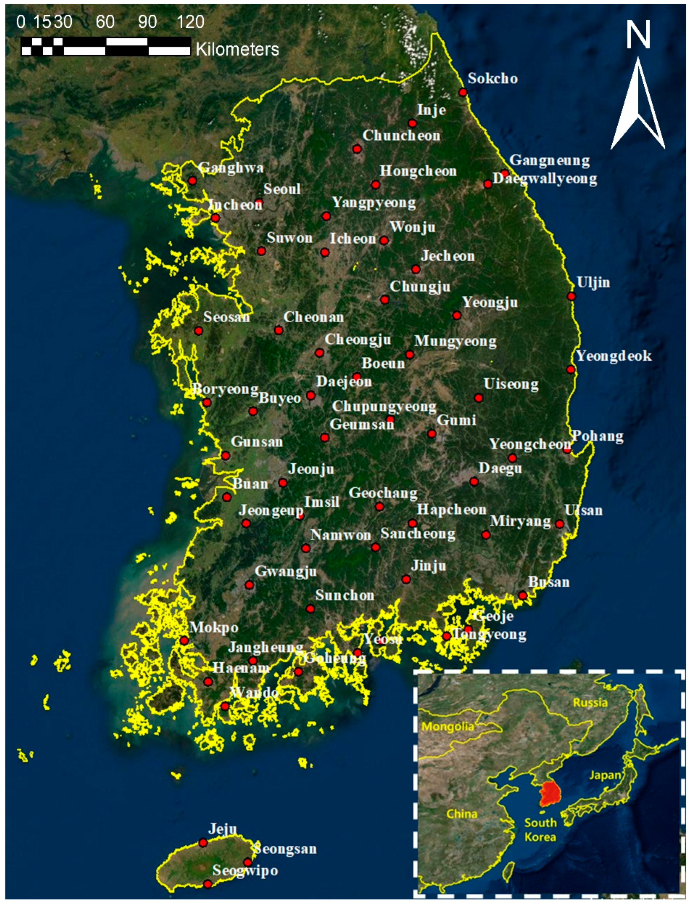
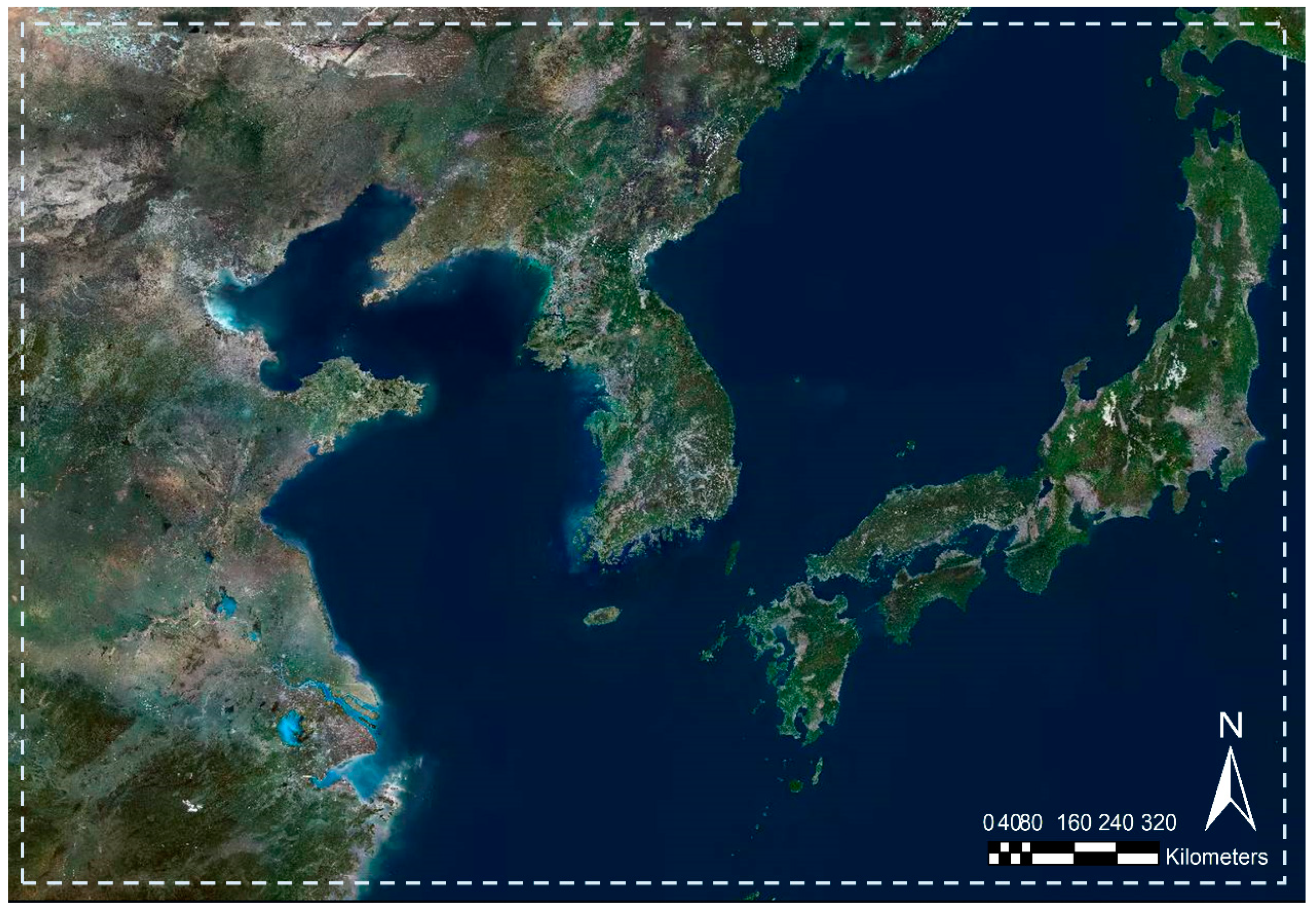
2.1. Study Area

Korea is located in the temperate climate zone of the mid-latitude (34–43° N) geographical area, and the four seasons of spring, summer, autumn, and winter are distinct. Since the three sides are surrounded by the sea, the climate is affected by the ocean, and the land is dominated by mountainous terrain. Therefore, high resolution climate models such as RCMs should be applied rather than low resolution climate models such as GCMs. The variability of river flow is very high since the average slope is relatively steep and the seasonal variation of precipitation is severe. The average annual precipitation varies widely depending on the region, but it is about 1500 mm, and 60–70% of the annual precipitation concentrates in the summer season. The geographical distribution of precipitation is characterized by geographical factors such as latitude and topography, and by meteorological factors such as atmospheric circulation and the arrangement of atmospheric pressure. In Korea, rainfall extremes are concentrated locally in summer, and the damage from rainfall extremes is increasing due to the effects of climate change.

2.2. Observed Data

Historical observed rainfall data for the period 1981–2010 measured in 60 weather stations across Korea have been provided by KMA (see Figure 1) [55]. The rainfall data have been recorded in ASOS. From this rainfall data, annual maximum rainfall intensities for 24 durations (1, 2, 3, 4, 5, 6, 7, 8, 9, 10, 11, 12, 13, 14, 15, 16, 17, 18, 19, 20, 21, 22, 23, and 24 h) were extracted.

2.3. Climate Change Scenarios

GCMs are the most important tools for estimating future precipitation for climate change scenarios, but they do not adequately simulate precipitation patterns on small spatial scales [56,57]. In order to overcome these limitations of GCMs, it is desirable to examine the changes of future rainfall using the results of RCMs, which dynamically down-scale GCM results into East Asia including Korea [58]. In this study, detailed climate change scenarios on the Korean peninsula (KOR-11), down-scaled in 12.5-km horizontal resolution into the East Asian region including the Korean peninsula from the results of GCMs, were used (see Figure 2). KOR-11 includes a total of 16 future climate ensembles from a combination of two GCMs including HadGEM2-AO (Hadley Centre Global Environmental Model version 2 coupled with the Atmosphere-Ocean, H2) and MPI-ESM-LR (Max Planck Institute Earth System Model-Low Resolution, ML) and four RCMs including MM5 (Meso-scale Model version 5; [59]), WRF(Weather Research and Forecasting model; [60]), RegCM4 (Regional Climate Model version 4; [61]), and RSM(Regional Spectral Model; [62]) under RCP 4.5 and 8.5 climate change scenarios. These models participated in the CORDEX-East Asia project [63]. Table 1 summarizes the future climate data used in this study.

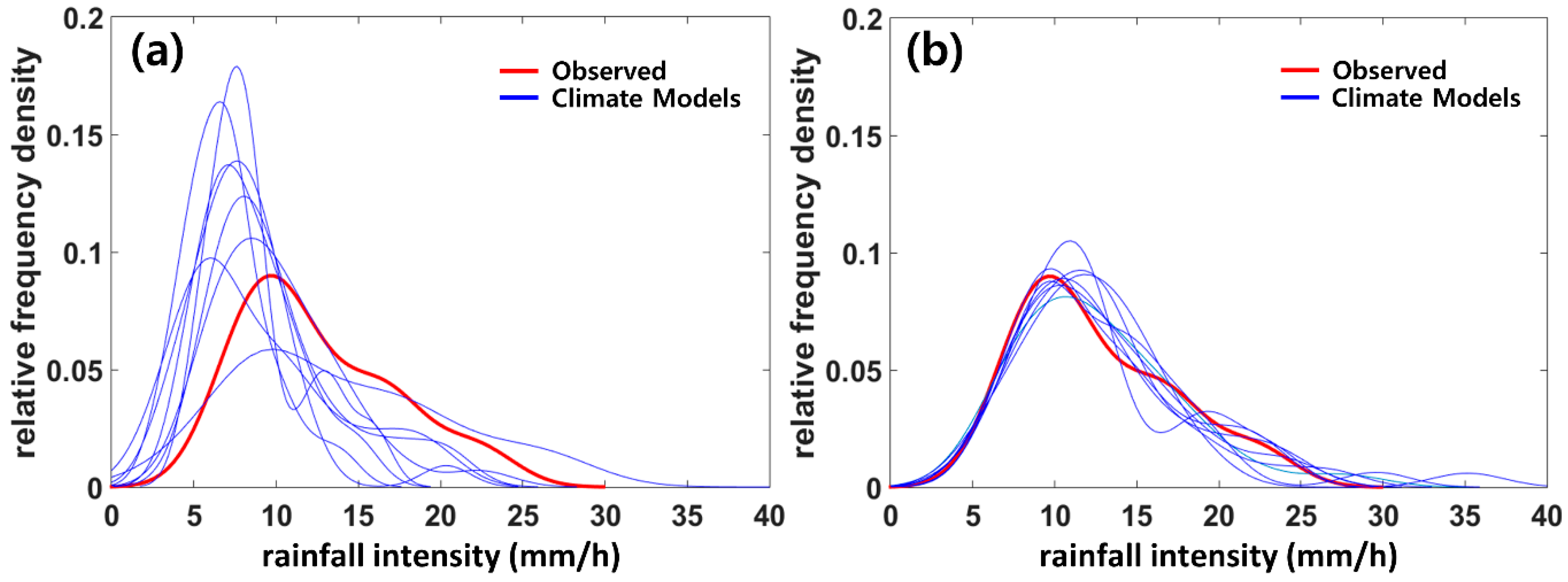
2.4. Bias Correction

Compared to GCMs, RCMs simulate local climate characteristics more closely in practice, but simulated precipitation still has many biases [64]. In addition, since RCMs are driven by using the output of GCMs as boundary conditions, the biases in GCMs are systematically transferred to RCMs. Hence, in order to utilize the results of RCMs in disaster prevention and adaptation policies for climate change in water and environment business, a bias-correction process for outputs from RCMs should be performed. A variety of bias-correction methods such as quantile mapping, quantile delta mapping, detected quantile mapping, change factor, and so on have been developed. First, as a result of temporarily estimating the future IDF curve using the above four bias-correction methods, there was little sensitivity of the future IDF curve to the bias correction method. Therefore, in this study, we corrected the bias using quantile mapping. Cannon et al. [65] warned that quantile mapping could inflate relative trends in extremes of precipitation, so we used a simple extrapolation technique proposed by Boé et al. [64] to prevent these problems in advance. The bias correction was performed on the annual maximum time series extracted for each duration.
The probability density function for quantile mapping is applied to the Generalized Extreme Value (GEV) distribution, and the parameters of the GEV distribution are estimated using the probability weighted moment method. However, since the GEV distribution has a limited range of shape parameters, the Gumbel distribution is applied instead when the GEV distribution is not suitable.

2.5. Scale-Invariance Method

Since the time resolution of a given future rainfall data is 3 h, temporal disaggregation is required to obtain the design rainfall intensity for various durations. In this study, scale-invariance method was applied. In case of future rainfall data of 24 h time resolution, the design rainfall intensity for the duration of less than 24 h can be calculated as shown in Equation (1) by using the method proposed by Choi et al. [58].
I d T = ( d 24 ) H × I 24 T ,
where I d T is the design rainfall intensity for the return period T years and duration d hours, I 24 T is the design rainfall intensity for the return period T years and duration 24 h, and H is the scale exponent. The scale exponent used in Equation (1) applies a single scale exponent obtained when examining the scale characteristics of the observed data. In other words, if future rainfall data of 24 h time resolution is given, it is assumed that the data of interest has a single scale characteristic. However, in case of future rainfall data of 3 h time resolution, various scale exponents can be applied for each duration interval by making full use of the multiple scale characteristics of the data. That is, given the design rainfall intensity I d 1 T of duration d 1 hours and the design rainfall intensity I d 2 T of duration d 2 hours (For example, d 1 = 3 h, d 2 = 6 h), the scale exponent H d 1 d 2 between duration d 1 hours and duration d 2 hours can be estimated as:
H d 1 d 2 =   ln ( I d 1 T / I d 2 T ) ln ( d 1 / d 2 ) ,
Using Equation (2), the design rainfall intensity of the duration d hours between duration d 1 hours and duration d 2 hours (e.g., d = 4 h or 5 h) can be estimated as follows:
I d T = ( d d 2 ) H d 1 d 2 × I d 2 T ,
Equations (2) and (3) are used to calculate the scale exponents H 3 6 h , H 6 9 h , …, H 21 24 h , respectively, and the design rainfall intensities for duration 4, 5, 7, 8, …, 19, 20, 22, 23 h. For more information, see Kim et al. [66].

3. Uncertainty of Future IDF Curves

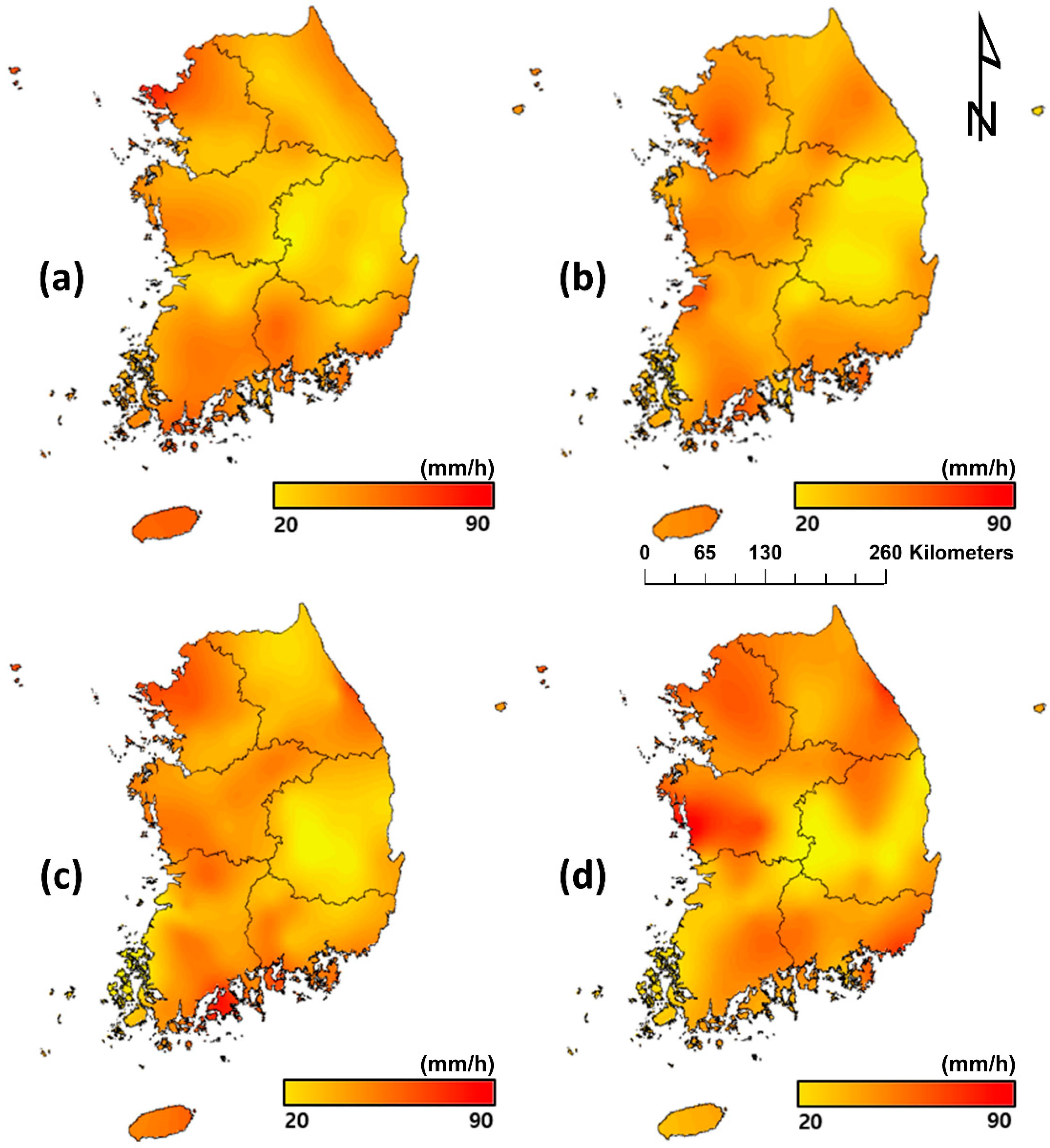
3.1. Bias-Correction Results

As a result, GEV distribution was applied to 35 out of 60 sites and Gumbel distribution was applied to the remaining 25 sites. In order to examine the effect of bias-correction, the empirical distribution of annual maximum rainfall intensity time series before and after the bias-correction at the Seoul site is shown in Figure 3, and Table 2 shows the mean values of the annual maximum rainfall intensity time series at the Seoul site before and after the bias-correction.
Comparing the frequency distributions before and after the bias-correction, it can be seen that the frequency distribution of the scattered GCM–RCM combination was bias-corrected similar to the frequency distribution of the observed values. As shown in Table 2, the difference between the mean of the observed annual maximum rainfall intensity time series and the mean of the corresponding bias-corrected time series is less than 0.1 mm/h, and the deviations between the mean values of annual maximum rainfall intensity series derived from all GCM–RCM combinations was also less than 0.5 mm/h. The tail of the distribution, which corresponds to rainfall extremes, also shows that the bias-corrected distribution follows the observed distribution relatively well (see Figure 3).
It is noteworthy that climate change affects rainfall intensity as well as rainfall frequency. If bias-correction is applied to the outputs from climate models, frequency information, especially in rainfall extremes, may be lost. However, this information loss is not considered in this study.

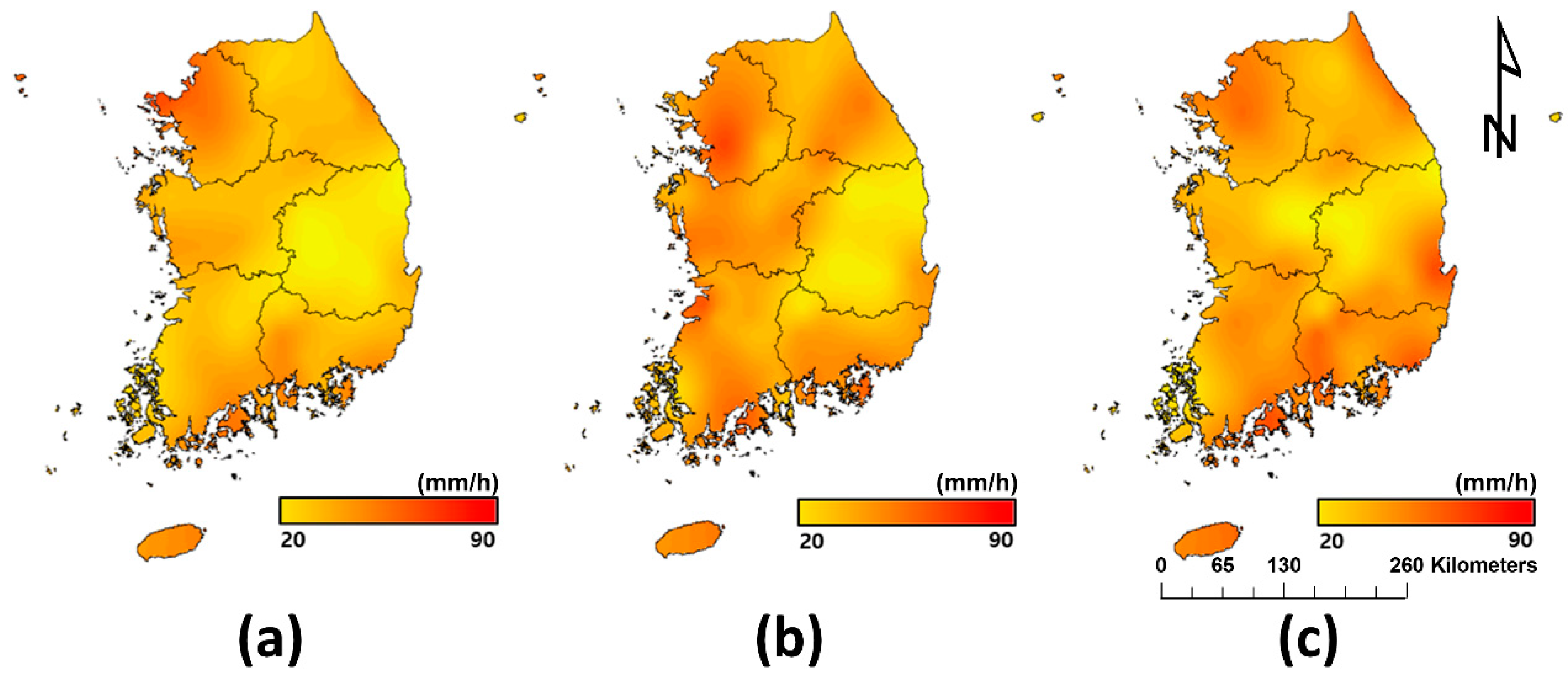
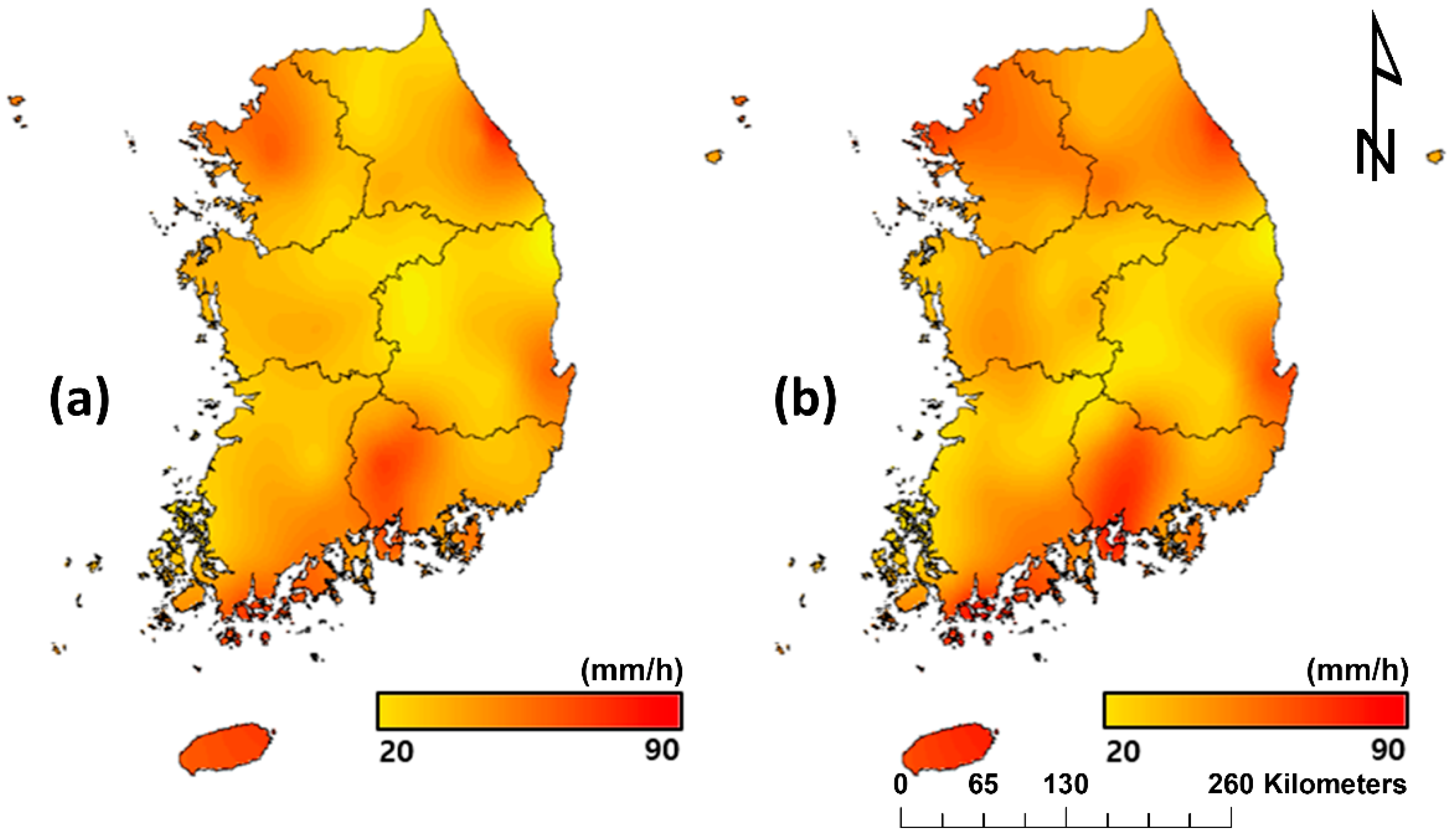
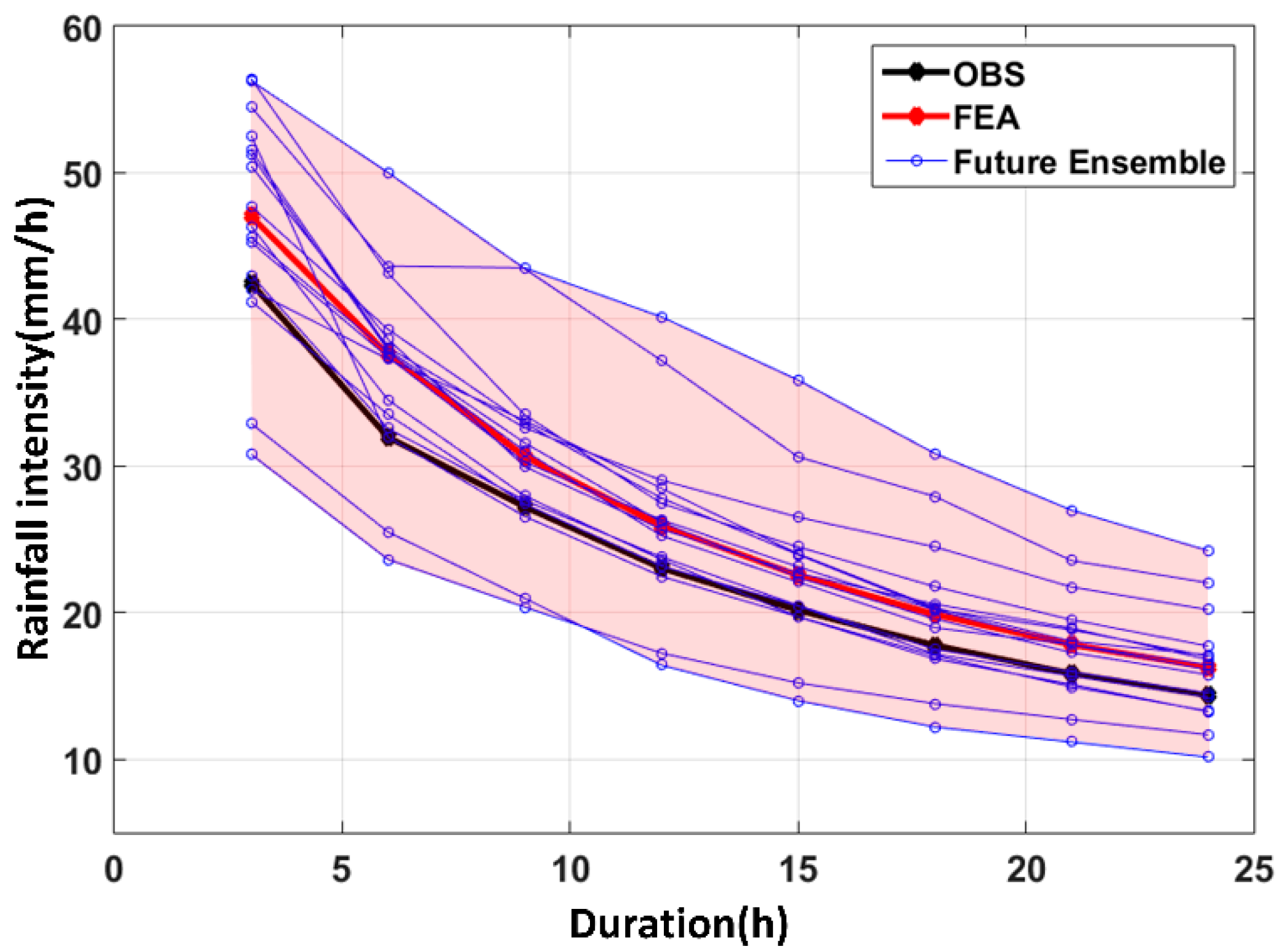
3.2. Future IDF Curves

Gumbel distribution was applied as a probability density function to estimate the design rainfall intensity. In Korea, the Gumbel distribution is used in principle to maintain the consistency of design practices [67]. Figure 4, Figure 5 and Figure 6 show the spatial distribution of design rainfall intensity derived from observations and future design rainfall intensity derived from several GCM/RCM/RCP combinations.
Figure 4 shows the future design rainfall intensity obtained when the RCP scenario and the RCM are the same (RCP 8.5-WRF) but the GCM is different. Figure 5 shows the future design rainfall intensity obtained when the RCP scenario and GCM are the same (RCP 8.5-ML) but the RCM is different. Figure 6 shows the future design rainfall intensity obtained when GCM and RCM are the same (H2-MM5) but RCP are different. Compared with the estimated design rainfall intensity (see Figure 4a) using observational data, the future design rainfall intensity is likely to increase overall regardless of the GCM/RCM/RCP combination, and a similar trend was found when applying the GCM/RCM/RCP combinations other than the combinations in Figure 4, Figure 5 and Figure 6. In fact, it would be reasonable to understand that this trend (that is, increase in rainfall extremes) has already been determined from the output of GCMs. In this study, two GCMs were used to dynamically force four RCMs. Therefore, the simulated tendency in GCMs is systematically transferred to RCMs.
Important points in Figure 4, Figure 5 and Figure 6 are that different future design rainfall intensity is estimated even if only one of the GCM/RCM/RCP combination is changed. This implies that there are many uncertainties in future rainfall extremes obtained from climate models [68]. This implies that although the mechanism of the local processes simulating rainfall extremes is the same (i.e., in the case of Figure 4 with the same RCM), when the boundary conditions driving the RCM are different (i.e., different GCMs are applied), different future design rainfall intensity is estimated. Conversely, if the boundary conditions driving the RCM are the same (i.e., in the case of Figure 5 with the same GCM), and if the mechanism of the local processes simulating rainfall extremes are different (i.e., different RCMs apply), it can be seen that the design rainfall intensity is estimated very differently. However, if the GCM/RCM combination is the same and the RCP scenario is different (see Figure 6), it can be found that the spatial distribution of estimated future design rainfall intensity is similar, although its value is different. This means that if the boundary conditions for RCM implementation are the same and the mechanism of the local process simulating rainfall extremes is the same, the quantitative change of extreme precipitation to greenhouse gas emission concentration is significantly different but there is not a relatively large difference in the spatial distribution of rainfall extremes. Also, as shown in Figure 6, it is analyzed that it cannot be said that the future design rainfall intensity with RCP 8.5 scenario emitting more greenhouse gases (and thus projecting higher surface air temperature rise) is necessarily greater than the future design rainfall intensity with RCP 4.5 scenario. On the whole, it is found that the RCP 4.5 scenario tends to show a larger design rainfall intensity.
However, if we look at the rate of change in design rainfall intensity by site, we can see that the results are difficult to explain. A quantitative analysis of the rate of change for duration 3 h and return period 30 years at the Busan site revealed −5.5% for ML-WRF-RCP 8.5 and 20.9% for H2-WRF-RCP 8.5 (see Figure 4). This is a very big difference, and even the sign is different. This deviation may be attributed to the different GCMs. However, it is found that this is not true if the same GCM is applied. In other words, even if both the GCM and RCP scenarios are the same (ML-RCP 8.5), it can be found that different RCMs produce very large deviations in rate of change (17.6% for MM5, −5.5% for WRF, 3.3% for RegCM4, and 37.6% for RSM, respectively, see Figure 5). This irregularity can still be found even if both GCM and RCM are the same (H2-MM5). In other words, different RCP scenarios can produce very large deviations in rate of change (−2.9% for RCP 8.5 and −17.5% for RCP 4.5, see Figure 6). Similar results can be obtained for different sites, different durations, or different return periods. In fact, such results that the reliability of the simulated (or estimated) future rainfall extremes from climate models are not high is not surprising (see [69] for further discussion).

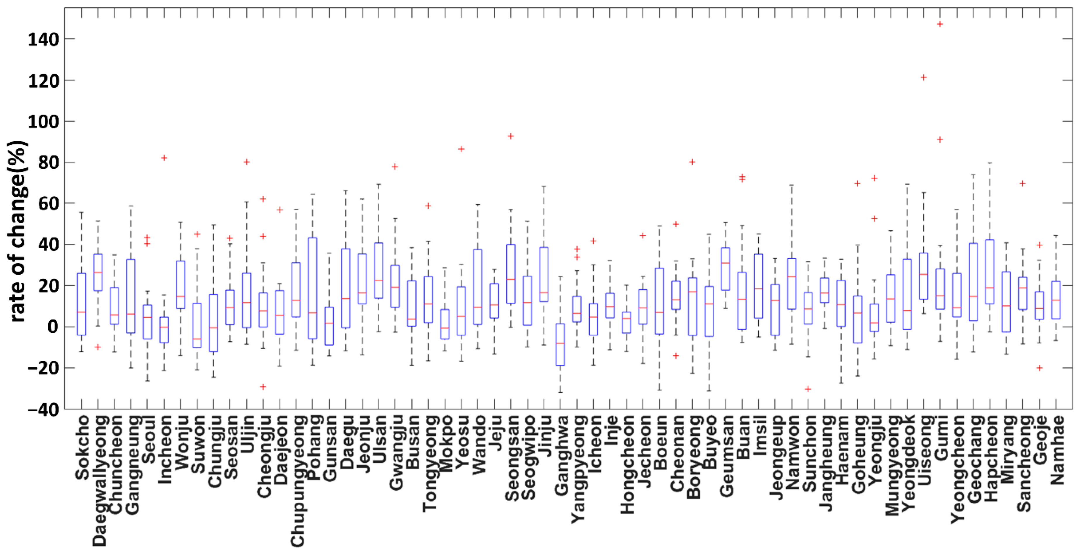
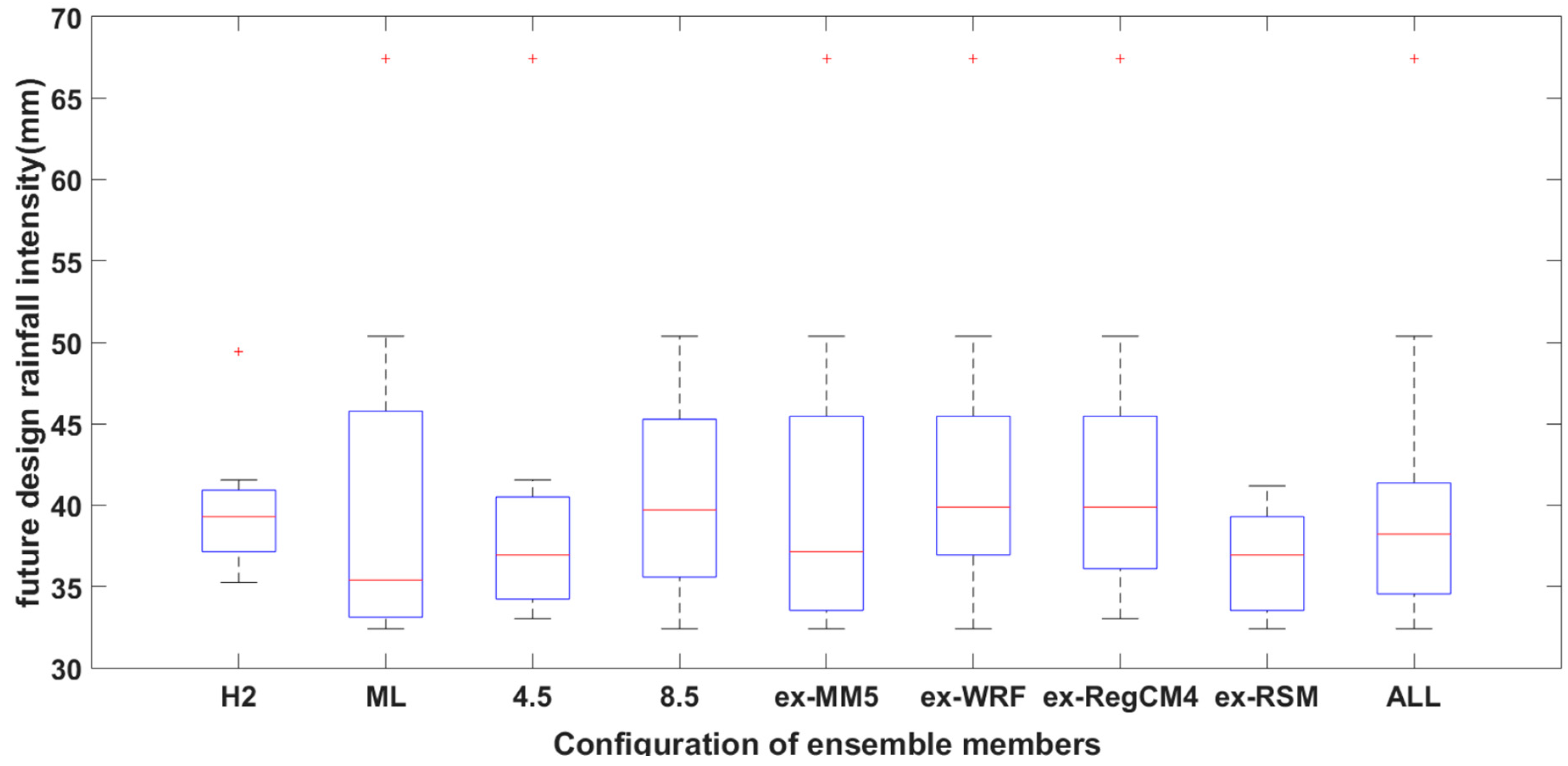
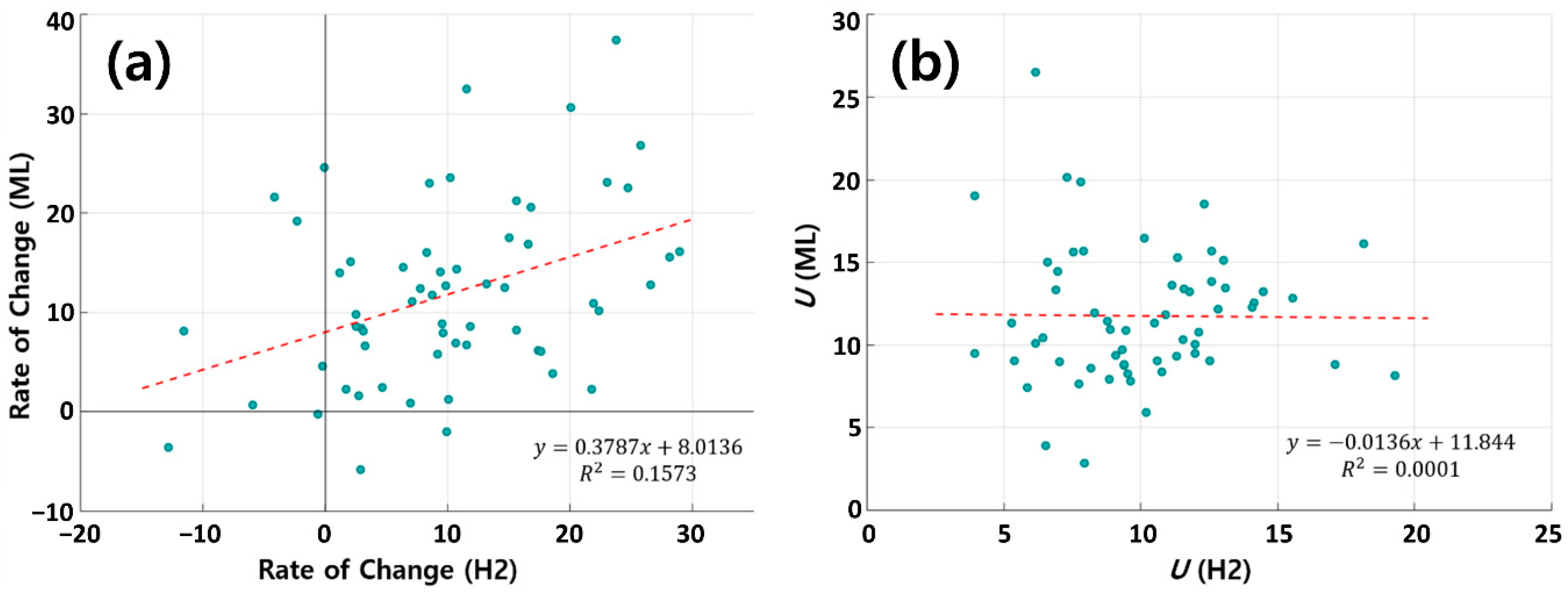
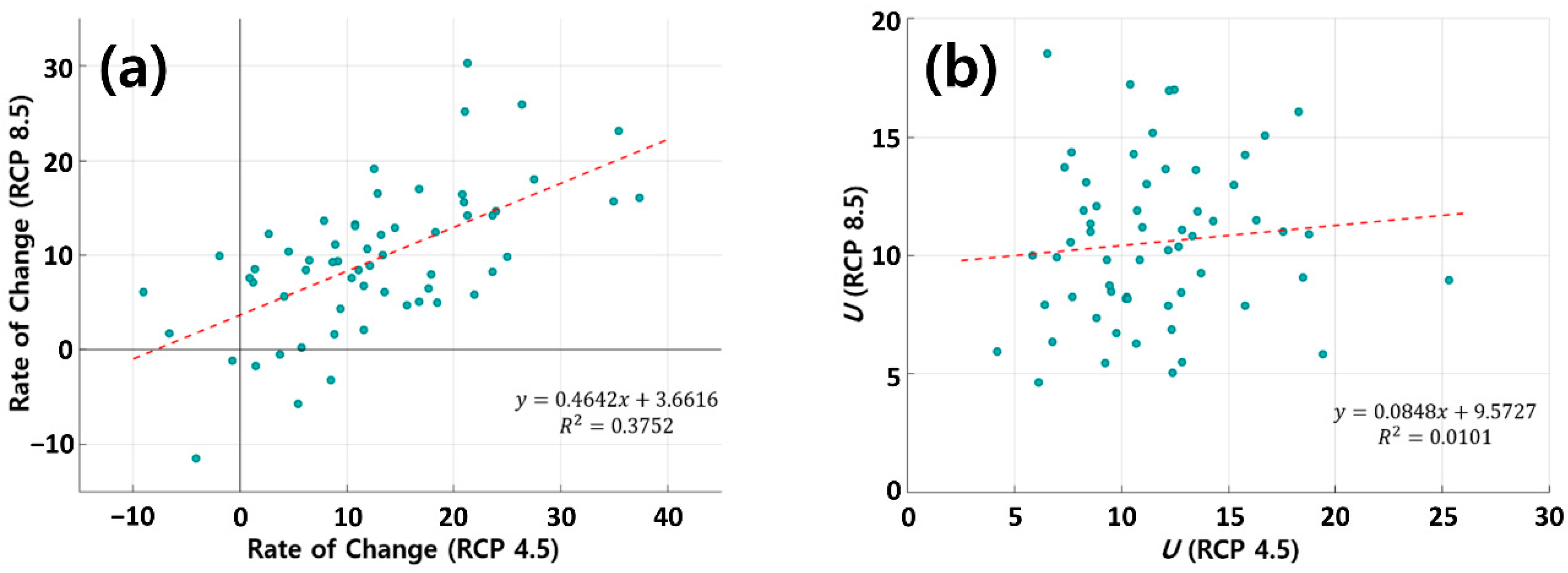
3.3. Rate of Change and Future Ensemble Average

In this study, 16 future design rainfall intensity ensembles (combination of 2 GCMs, 4 RCMs, and 2 RCPs) were estimated for various return periods T years and various durations d hours at various sites. Their median for each return period T years and duration d hours is defined as Future Ensemble Average (FEA) and the rate of change R c (%) of future design rainfall intensity is defined as follows:
R c = F E A ( T , d )   O B S ( T , d ) O B S ( T , d ) ,
where FEA(T,d) is the median of future design rainfall intensity ensembles of the return period T years and the duration d hours, and OBS(T,d) is the estimated design rainfall intensity from the corresponding observations. Figure 7 shows 16 future design rainfall intensity ensembles and their FEA at the Haenam site. For reference, the rate of change of the future design rainfall intensity for the return period 30 years and duration 3 h estimated from 16 ensembles at the Haenam site was calculated to be 10.7%. This means that the design rainfall intensity may increase by about 11% compared with the present.
However, as shown in Figure 7, due to the large difference between estimated future rainfall intensities depending on which GCM/RCM/RCP combination is applied, it is hard to say that the reliability for an increase in design rainfall intensity of about 11% on FEA basis is sufficiently secured. As shown in the boxplot of Figure 8a, the Inter-Quantile Range (IQR) of the rate of change contains the portion where the rate of change is zero. This implies that the differences between the ensembles are relatively larger than the rate of change of the FEA, which makes it difficult to see that future design rainfall intensity increases significantly. Figure 8b shows the boxplot at the Geumsan site. Unlike the Haenam site, the rate of change at the Geumsan site is relatively larger than the differences between the ensembles. Therefore, the risk that the future design rainfall intensity will increase at the Geumsan site can be more clearly presented to policymakers who establish climate change adaptation policies.

3.4. Uncertainty Analysis of Future IDF Curves

As we have seen, the future design rainfall intensity will depend on which GCM/RCM/RCP combination is applied, so the difference between ensemble members of future design rainfall intensity can be defined as the uncertainty of future design rainfall intensity estimation. In this study, the uncertainty of the future design rainfall intensity was defined as U = 0.6745 × C V ( T , d ) using the coefficient of variation C V ( T , d ) of ensemble members applied to FEA. This means that the uncertainty is defined as the Inter-Quantile Range (IQR) of ensemble members. For example, when analyzing uncertainty using all GCM/RCM/RCP combinations, the coefficient of variation of 16 future ensembles will be used. This allows quantification of uncertainties for various GCM/RCM/RCP combinations by site, duration, and return period.
In this case, various analyses can be attempted by varying the method of constructing the ensemble members included in the calculation of the FEA. The most commonly applied method is to calculate the FEA considering all available ensemble members. That is, in this study, FEA can be calculated using all 16 future ensembles, and corresponding rate of change and its uncertainty can be presented. In addition, FEA can be calculated using 8 future ensembles for each GCM, and the rate of change and its uncertainty corresponding to the applied GCM can be presented. In a similar manner, a rate of change and its uncertainty corresponding to the RCM applied, or a rate of change and its uncertainty corresponding to the applied RCP may be presented, respectively.
This section looks at the rate of change of future IDF curves for GCM/RCM/RCP combination and the uncertainty involved. The FEA calculated using all 16 ensemble members and its uncertainty are shown in Figure 9 The number of sites where the FEA is greater than the IQR of the ensembles (i.e., 0.6745 × C V ( T , d ) ) is 28 out of a total of 60 sites. In other words, 47% of the analyzed sites can be credibly presented to decision makers that future design rainfall intensity is likely to increase.
Figure 10 shows a boxplot of the rate of change for how ensemble members are constructed. In the configuration of ensemble members classified by GCM as H2 and ML in the figure, the rate of change and uncertainty of future design rainfall intensity were estimated by using 8 future ensembles for each GCM. In the configuration of the ensembles classified by the RCP, the rate of change and uncertainty of the future design rainfall intensity were estimated by using 8 future ensembles for each RCP as in the configuration separated by GCM. Analyzing the rate of change and uncertainty of future design rainfall intensity using ensemble members identified by RCM needs to be examined in a slightly different way. Since there are 4 RCMs applied in this study, the rate of change and uncertainty of future design rainfall intensity are calculated using only 4 ensemble members when analyzed by RCM. Since the number of ensemble members for uncertainty analysis was considered to be insufficient, this study constructed ensemble members excluding ensembles derived from one specific RCM (for example, MM5) among all ensembles derived from all RCMs (for example, ex-MM5 in the figure). If the uncertainty in the ensemble configuration where the MM5 is excluded is lower than the uncertainty in the configuration in which all the RCMs are applied, this means that the uncertainty is greatly increased due to ensemble members derived from MM5. Of course, such a method has the disadvantage that it cannot directly represent the rate of change and uncertainty of RCM, but it can be indirectly grasped the contribution of uncertainty by RCM.
At the Uiseong site, ML showed clearly higher uncertainty than H2. The uncertainty of RCP 4.5 is lower than that of RCP 8.5, but there is an outlier in the ensembles of RCP 4.5 (red + in Figure 10). Therefore, the uncertainty of RCP 4.5 ( U = 18.8%) becomes much larger than the uncertainty of RCP 8.5 ( U = 10.9%) when the outlier is considered. In addition, the uncertainty was greatly reduced in configurations except the ensembles derived using RSM, and no outlier was found. That is, at the Uiseong site, it can be seen that the ensembles derived from the combinations containing ML/RSM/RCP 8.5 present future design rainfall intensities that are different from the ensembles derived from other combinations. This fact implies that using many ensembles unconditionally is not necessarily an absolute way to reduce uncertainty.
By using 8 future ensembles for each GCM, the rate of change and uncertainty of future design rainfall intensity by GCM can be estimated. To see the difference between two different GCMs at the same site, the FEA and its uncertainty U of the rate of change using each GCM-specific ensemble members are shown in Figure 11. Overall, the rates of change derived from ML are calculated to be larger than the rates of change derived from H2, and ML is larger than H2 in terms of differences between ensemble members. However, since there are many sites where the rate of change calculated from H2 is larger than the value from ML and the determinant coefficient of the linear regression line is low as 0.1573, it is concluded that the future design rainfall intensity derived by applying ML is not necessarily larger than future design rainfall intensity derived by H2. In the case of uncertainty, there was little correlation between the two GCMs. In other words, it can be said that it is difficult to see what GCM is applied to determine the difference in future design rainfall intensity. Although the future design rainfall intensity is calculated differently depending on which GCM is applied, the GCMs carried out up to the dynamics down-scale in Korea have only two of ML and H2. Therefore, it would be the most feasible and realistic alternative to investigate changes in future design rainfall intensity using all of the GCMs rather than excluding one GCM.
As with GCM, the rate of change and uncertainty of future design rainfall intensity for each RCP can be estimated using 8 future ensembles for each RCP. Figure 12 shows the same figure in Figure 11, except that RCP is applied as a control variable instead of GCM. Slightly different from the results in GCM, there are some correlations between future design rainfall intensity of two RCP configurations. It can be confirmed that the design rainfall intensity under the RCP 4.5 scenario tends to be larger than the design rainfall intensity under the RCP 8.5 scenario, but it is observed that only 38 sites out of 60 sites (63%) follow this tendency. In other words, it can still be said that it is difficult to see what RCP has been applied to determine future design rainfall intensity differences. Although future design rainfall intensities are estimated differently depending on what RCP is applied, there are only two RCP scenarios, 4.5 and 8.5, applied in this study. Therefore, it would be most feasible to investigate the future design rainfall intensity using both RCP scenarios rather than looking at future extreme rainfall by excluding one RCP scenario or separating the two scenarios. In terms of uncertainty, RCP 4.5 is found to be larger than RCP 8.5, but it is still difficult to see any relationship between uncertainties in the two scenarios. Also, it is possible to find sites with different directions in rate of change depending on the scenario, but it is difficult to see that the sign change of the rate of change is meaningful because the rate of change is relatively smaller than the uncertainty.
The rate of change and uncertainty of future design rainfall intensity for ensemble members identified by the RCM can be analyzed in a different way than in GCM and RCP. Table 3 shows the rate of change and its uncertainty when all 16 ensemble members are applied, and the rate of change and its uncertainty when the ensemble members derived from a specific RCM are excluded. It can be found that the average of the FEAs and the corresponding uncertainties of the rates of change at all sites are approximately 11% and 11%, respectively, regardless of whether all RCMs are applied or whether one RCM is excluded.
However, when we look at each site separately, we find interesting classification criteria. From a relative comparison of FEA with its uncertainty, the change (increase or decrease) may be considered significant if the FEA is greater than its uncertainty, or the change may be treated as meaningless if not. Therefore, the meaning of the color shown in Table 3 can be summarized as follows:
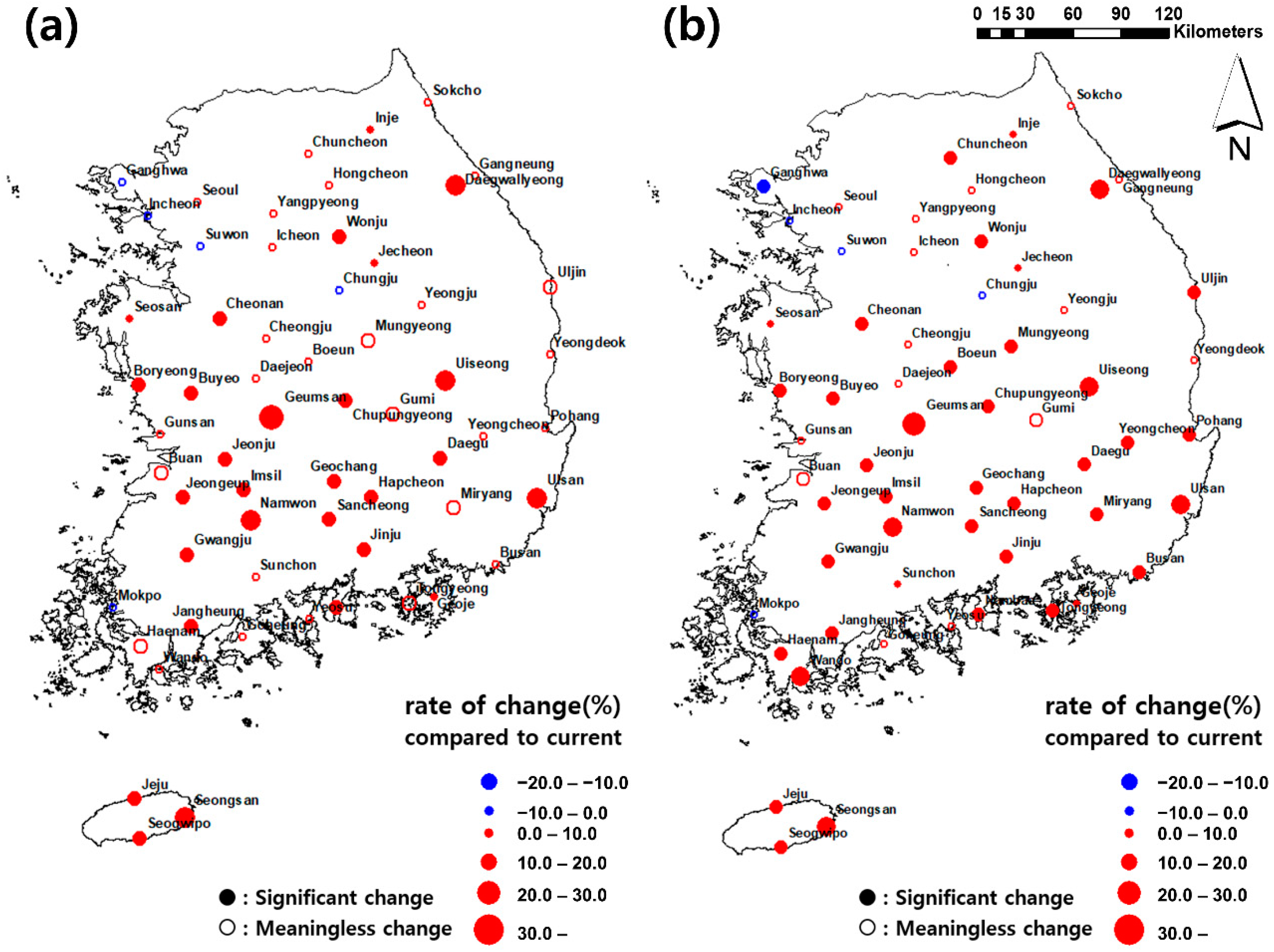
  • Red: Sites that show a significant increase when applying all RCMs, i.e., sites where FEA calculated by applying all RCMs is larger than its uncertainty. Future design rainfall intensity at these sites is likely to be higher than current design rainfall intensity.
  • Green: In these sites, FEA increases significantly when all RCMs are applied, but when one RCM is excluded, the increase in FEA is meaninglessly changed. Since uncertainty has increased by excluding the RCM, it can be seen that the RCM labeled Green contributes to reducing the uncertainty in future design rainfall intensity estimates. It can be seen that most of the sites marked Green are sites with little difference between FEA and uncertainty among sites marked Red. In Table 3, the RCMs marked Green are 2 sites for MM5, 6 sites for WRF, 3 sites for RegCM4, and 2 sites for RSM. From this, it can be seen that the uncertainties of the three RCMs are relatively larger than those of WRF.
  • Orange: These sites show a non-significant increase in FEA when all RCMs are applied, but FEA changes to a significant increase if one specific RCM is excluded. As can be seen from the Uljin site, since the FEA is larger than its uncertainty if the ensemble members derived from a particular RCM (e.g., MM5) are excluded, the RCM marked with Orange contributes to increasing the uncertainty. In Table 3, there are 5 sites in MM5, 3 sites in WRF, 6 sites in RegCM4, and 7 sites in RCM indicated by Orange. Consistent with the analysis in 2), it can be seen that the uncertainties of RCMs other than WRF are relatively larger. It is worth noting that RCMs can be identified for each site with a high level of uncertainty rather than a comparison of indirect uncertainty measures between RCMs. This can be used as a way to reduce the uncertainty in estimating future design rainfall intensity, which will be discussed in more detail in the next section.
  • Blue: In this site, FEA shows a meaningless decrease when all RCMs are applied, but when one specific RCM is excluded, FEA is converted to a significant decrease. There are 5 sites (blue text in Table 3) in which the future design rainfall intensity is less than the current design rainfall intensity, but none of them showed significant decrease when all RCMs were applied. However, it can be seen that the Ganghwa site shows a significant decrease when RegCM4 is excluded. In Korea, it has been reported that rainfall extremes will increase in the future in most studies, and in this study, it is general that rate of change also increases in most sites. Therefore, the decrease in FEA indicates that the variance of the design rainfall intensity between ensemble members is very large. From this point of view, a significant decrease at the Ganghwa site may need to be treated more carefully in the future.

4. Discussion

So far, we have quantified the rate of change and uncertainty of future design rainfall intensity in various ways. Through this, numerical presentation of rate of change and its uncertainty of future design rainfall intensity at various sites throughout Korea will be a meaningful result. However, the ultimate goal of the study of rainfall extremes in light of climate change will be how to include these uncertainties in climate change adaptation policies. In this section, we use the results derived from this study to deal with ways to reduce the uncertainty of the future design rainfall intensity and to reasonably reflect the climate change adaptation policy.
As shown in Table 3, it can be seen that unconditionally using many ensemble members does not necessarily reduce uncertainty. If so, we will have to figure out which ensemble members to exclude. GCMs and RCPs occupy 8 combinations out of a total of 16 combinations. In other words, excluding one GCM or RCP from the FEA and its uncertainty estimation procedure means that half of the existing ensemble members are lost. This was judged not to be a good way to look at the uncertain future. Therefore, we focus on four RCMs in this study because 12 ensemble members can still be used, even if one RCM is excluded.
As can be seen in Table 3, the number of red sites with a significant increase in FEA from ensembles derived from applying all RCMs is 29, which means that future design rainfall intensity is significantly higher at about 49% of the 60 sites. The remaining 31 sites are so uncertain that changes are not likely to be significant. We believe that if we deviate from the usual belief that the same ensembles should be applied to all sites, we can reduce the uncertainty of 31 sites individually. That is, by excluding the ensembles derived from a particular RCM that significantly contribute to the uncertainty of a site, the uncertainty contained in the FEA could be reduced. Since the more climate model combinations we can use, the smaller the impact of a particular ensemble on the FEA, there is no argument that increasing the number of climate model combinations is the most fundamental alternative to reducing uncertainty. In reality, however, increasing the number of climate model combinations is very difficult, so excluding specific ensemble from the ensembles available at the current level may be a more realistic alternative. When one RCM is excluded, the number of orange sites that change to a significant increase is 13. A total of 42 sites, combined with 29 red sites already showing a significant increase, can be designated as sites with increased future design rainfall intensity. This accounts for 70% of all 60 sites. Figure 13 shows FEA using ensembles derived from all RCMs (Figure 13a) and FEA in configurations except for ensembles derived from a specific RCM using the above method (Figure 13b).
Figure 13a consists of 29 sites with significant increases, 26 sites with insignificant increases, and 5 sites with no significant decreases. On the other hand, in Figure 13b, which is the result of removing one particular RCM that causes large uncertainties, 13 sites were additionally identified as sites that are expected to show a significant increase, and one site has been added to a site where FEA is significantly decreased. In this way, since selective application of RCMs at each site effectively utilizes the future climate data obtained from various climate models and at the same time reduces the difference between the ensembles derived from various future climate data, it is expected that it will provide more reasonable and persuasive results when establishing climate change adaptation policy.
Finally, the relationship between FEA and its uncertainty for duration and return period was examined. First, to examine the future design rainfall intensity for duration, we plot boxplots of rates of change by duration based on return period 30 years at the Seoul site (Figure 14a). The rate of change for the duration was analyzed as not showing a specific pattern, but in short durations (for example, 3 h and 6 h), sites with some changes in the sign of the FEA were found. Overall, the uncertainty of FEA in duration 3 h was larger than that of FEAs in other durations, although it was not included in the paper. This is also confirmed by the fact that there are 3 outliers in duration 3 h at the Seoul site.
Similar results for the return period are shown in Figure 14b. Overall, as the return period increases, the future design rainfall intensity is likely to increase, but the uncertainty corresponding to the FEA does not increase as much.

5. Conclusions

In this study, future IDF curves were estimated and corresponding uncertainties were quantified using future rainfall data from various RCMs applicable to Korea. Future rainfall data were obtained from combinations of two GCMs (MPI-ESM-LR and HadGEM2-AO) and four RCMs (MM5, WRF, RegCM4, and RSM) based on two climate change scenarios (RCP 4.5 and 8.5). From the RCM simulation data, data corresponding to ASOS 60 observation sites operated by KMA were extracted and the annual maximum time series of the extracted data was bias-corrected using quantile mapping. Using the derived future IDF curves, various FEAs of rates of change for design rainfall intensity and their uncertainties were calculated for each site, return period, and duration.
Analyses of ensembles of rate of change derived from the same GCM showed that the future design rainfall intensity derived from MPI-ESM-LR was estimated to be larger than that derived from HadGEM2-AO, and the uncertainty was also larger in MPI-ESM-LR. Considering the ensembles of rate of change derived under the same RCP climate change scenario, the future design rainfall intensity derived from RCP 4.5 was estimated to be larger than that simulated from RCP 8.5, and the uncertainty was also greater at RCP 4.5. However, whether the GCM or which RCP is applied does not determine the difference in future design rainfall intensity, and very different results are obtained for each point. Therefore, it would be meaningless to represent the future rate of change for GCM or for RCP as an exact number. Given the realistic constraints of only two GCMs dynamically down-scaled on the Korean Peninsula and available only on RCP 45 and 85 climate change scenarios, it was considered to be the most feasible and realistic alternative to analyze the changes of future design rainfall intensity using both GCMs and two RCPs rather than excluding one GCM or RCP.
As a result of estimating the rate of change and uncertainty of future design rainfall intensity by constructing ensemble members excluding ensembles derived from one specific RCM among all ensembles derived from all RCMs, using unconditionally many ensembles does not necessarily reduce uncertainty. By excluding the ensembles derived from a particular RCM that contributed significantly to site-specific uncertainties, the uncertainty involved in FEA could be reduced. Through this, it was possible to identify a significant change in future design rainfall intensity at 43 out of 60 sites. In other words, by selectively applying future ensembles derived from RCMs, we were able to effectively utilize future climate data from various climate models, while at the same time mitigating the differences between ensembles derived from various future climate data. This reduction in uncertainty is expected to contribute to providing clearer and more persuasive results to policymakers in developing climate change adaptation policies.
As the return period increases, the rate of change of future design rainfall intensity increases, but uncertainty does not appear to be significantly responsive to changes in return period. However, as a result of analyzing FEA and its uncertainty of future design rainfall intensity for duration, the uncertainty of future design rainfall intensity of short duration was relatively high. Therefore, it is concluded that the future design rainfall intensity for durations below the temporal resolution of RCMs is still limited.
This study focused on the uncertainties caused by GCMs and RCMs ensemble in future projections of design rainfall depth. However, extreme value analysis involves very large uncertainties related to the parameters of probability distributions resulting from small numbers of data. Due to the uncertainties included in parameter estimation of the applied probability distribution, it may be necessary to further discuss whether the differences between ensembles obtained from GCMs or RCMs are statistically significant.

Author Contributions

Conceptualization, K.K. and S.K.; Data curation, D.-H.C.; Formal analysis, K.K.; Investigation, K.K., J.C. and O.L.; Methodology, K.K. and S.K.; Project administration, S.K.; Resources, D.-H.C.; Supervision, S.K.; Validation, D.-H.C. and S.K.; Visualization, K.K., J.C. and O.L.; Writing—original draft, K.K.; Writing—review & editing, S.K. All authors have read and agreed to the published version of the manuscript.

Funding

This research was funded by Korea Environmental Industry and Technology Institute, grant number 2016000200002.

Acknowledgments

This work was supported by Korea Environment Industry & Technology Institute (KEITI) through Public Technology Program based on Environmental Policy Project, funded by Korea Ministry of Environment (MOE) (2016000200002).

Conflicts of Interest

The authors declare no conflict of interest.

References

  1. Handmer, J.; Honda, Y.; Kundzewicz, Z.W.; Arnell, N.; Benito, G.; Hatfield, J.; Mohamed, I.F.; Peduzzi, P.; Wu, S.; Sherstyukov, B.; et al. Changes in impacts of climate extremes: Human systems and ecosystems. In Managing the Risks of Extreme Events and Disasters to Advance Climate Change Adaptation Special Report of the Intergovernmental Panel on Climate Change; Field, C.B., Barros, V., Stocker, T.F., Qin, D., Dokken, D.J., Ebi, K.L., Mastrandrea, M.D., Mach, K.J., Plattner, G.-K., Allen, S.K., et al., Eds.; Cambridge University Press: Cambridge, UK; New York, NY, USA, 2012; pp. 231–290. [Google Scholar]
  2. Intergovernmental Panel on Climate Change (IPCC). Climate Change 2014: Synthesis Report; Contribution of Working Groups I, II and III to the Fifth Assessment Report of the Intergovernmental Panel on Climate Change; Core Writing Team, Pachauri, R.K., Meyer, L.A., Eds.; IPCC: Geneva, Switzerland, 2014. [Google Scholar]
  3. Kharin, V.V.; Zwiers, F.W.; Zhang, X.; Hegerl, G.C. Changes in temperature and precipitation extremes in the IPCC ensemble of global coupled model simulations. J. Clim. 2007, 20, 1419–1444. [Google Scholar] [CrossRef] [Green Version]
  4. Berg, N.; Hall, A. Increased interannual precipitation extremes over California under climate change. J. Clim. 2015, 28, 6324–6334. [Google Scholar] [CrossRef]
  5. Loo, Y.Y.; Billa, L.; Singh, A. Effect of climate change on seasonal monsoon in Asia and its impact on the variability of monsoon rainfall in Southeast Asia. Geosci. Front. 2015, 6, 817–823. [Google Scholar] [CrossRef] [Green Version]
  6. Burt, T.; Boardman, J.; Foster, I.; Howden, N. More rain, less soil: Long-term changes in rainfall intensity with climate change. Earth Surf. Process. Landf. 2016, 41, 563–566. [Google Scholar] [CrossRef] [Green Version]
  7. Intergovernmental Panel on Climate Change (IPCC). Global climate projections. In Climate Change 2007: The Physical Science Basis; Solomon, S., Qin, D., Manning, M., Chen, Z., Marquis, M., Averyt, K.B., Tignor, M., Miller, H.L., Eds.; Cambridge University Press: Cambridge, UK; New York, NY, USA, 2007. [Google Scholar]
  8. Coles, S.; Pericchi, L.R.; Sisson, S. A fully probabilistic approach to extreme rainfall modeling. J. Hydrol. 2003, 273, 35–50. [Google Scholar] [CrossRef]
  9. Goswami, B.N.; Venugopal, V.; Sengupta, D.; Madhusoodanan, M.S.; Xavier, P.K. Increasing trend of extreme rain events over India in a warming environment. Science 2006, 314, 1442–1445. [Google Scholar] [CrossRef] [Green Version]
  10. Valeo, C.; Xiang, Z.; Bouchart, F.C.; Yeung, P.; Ryan, M.C. Climate change impacts in the Elbow River watershed. Can. Water Resour. J. 2007, 32, 285–302. [Google Scholar] [CrossRef]
  11. Robinson, K.L.; Valeo, C.; Ryan, M.C.; Chu, A.; Iwanyshyn, M. Modelling aquatic vegetation and dissolved oxygen after a flood event in the Bow River, Alberta, Canada. Can. J. Civ. Eng. 2009, 36, 492–503. [Google Scholar] [CrossRef]
  12. He, J.; Valeo, C.; Chu, A.; Neumann, N.F. Stormwater quantity and quality response to climate change using artificial neural networks. Hydrol. Process. 2011, 25, 1298–1312. [Google Scholar] [CrossRef]
  13. Climat.Gov. Available online: https://www.climate.gov/news-features/blogs/beyond-data/2017-us-billion-dollar-weather-and-climate-disasters-historic-year (accessed on 26 May 2018).
  14. Harris County Flood Warning System. Available online: https://www.harriscountyfws.org/GageDetail/Index/1730 (accessed on 26 May 2018).
  15. Van Oldenborgh, G.J.; Van Der Wiel, K.; Sebastian, A.; Singh, R.; Arrighi, J.; Otto, F.; Haustein, K.; Li, S.; Vecchi, G.; Cullen, H. Attribution of extreme rainfall from Hurricane Harvey, August 2017. Environ. Res. Lett. 2017, 12, 124009. [Google Scholar] [CrossRef]
  16. Risser, M.D.; Wehner, M.F. Attributable human-induced changes in the likelihood and magnitude of the observed extreme precipitation during hurricane Harvey. Geophys. Res. Lett. 2017, 44, 12457–12464. [Google Scholar] [CrossRef] [Green Version]
  17. Guhathakurta, P.; Sreejith, O.P.; Menon, P.A. Impact of climate change on extreme rainfall events and flood risk in India. J. Earth Syst. Sci. 2011, 120, 359. [Google Scholar] [CrossRef]
  18. McCuen, R.H. Hydrologic Analysis and Design; Prentice-Hall: Englewood Cliffs, NJ, USA, 1989; pp. 143–147. [Google Scholar]
  19. Prodanovic, P.; Simonovic, S.P. Development of rainfall intensity duration frequency curves for the City of London under the changing climate. In Water Resources Research Report; Department of Civil and Environmental Engineering, The University of Western Ontario: London, ON, Canada, 2007. [Google Scholar]
  20. Choi, J.; Lee, O.; Kim, S. Analysis of the effect of climate change on IDF curves using scale-invariance technique: Focus on RCP 8.5. J. Korea Water Resour. Assoc. 2016, 49, 995–1006. [Google Scholar] [CrossRef]
  21. Koutsoyiannis, D.; Kozonis, D.; Manetas, A. A mathematical framework for studying rainfall intensity-duration-frequency relationships. J. Hydrol. 1998, 206, 118–135. [Google Scholar] [CrossRef]
  22. Solaiman, T.A.; Simonovic, S.P. Development of probability based intensity-duration-frequency curves under climate change. In Water Resources Research Report; Department of Civil and Environmental Engineering, The University of Western Ontario: London, ON, Canada, 2011. [Google Scholar]
  23. Mirhosseini, G.; Srivastava, P.; Stefanova, L. The impact of climate change on rainfall Intensity–Duration–Frequency (IDF) curves in Alabama. Reg. Environ. Chang. 2013, 13, 25–33. [Google Scholar] [CrossRef]
  24. Shrestha, A.; Babel, M.; Weesakul, S.; Vojinovic, Z. Developing Intensity–Duration–Frequency (IDF) curves under climate change uncertainty: The case of Bangkok, Thailand. Water 2017, 9, 145. [Google Scholar] [CrossRef] [Green Version]
  25. Li, X.; Wang, X. Analysis of variability and trends of precipitation extremes in Singapore during 1980–2013. Int. J. Climatol. 2018, 38, 125–141. [Google Scholar] [CrossRef]
  26. Balling, R.C.; Kiany, K.; Sadegh, M.; Sen Roy, S.; Khoshhal, J. Trends in extreme precipitation indices in Iran: 1951–2007. Adv. Meteorol. 2016, 2016, 2456809. [Google Scholar] [CrossRef] [Green Version]
  27. Rahmani, V.; Hutchinson, S.L.; Harrington, J.A.; Shawn Hutchinson, J.M. Analysis of frequency and magnitude of extreme rainfall events with potential impacts on flooding: A case study from the central United States. Int. J. Climatol. 2016, 36, 3578–3587. [Google Scholar] [CrossRef]
  28. Paschalis, A.; Molnar, P.; Fatichi, S.; Burlando, P. A stochastic model for high-resolution space-time precipitation simulation. Water Resour. Res. 2013, 49, 8400–8417. [Google Scholar] [CrossRef]
  29. Fatichi, S.; Ivanov, V.Y.; Caporali, E. Simulation of future climate scenarios with a weather generator. Adv. Water Resour. 2011, 34, 448–467. [Google Scholar] [CrossRef]
  30. Li, X.; Babovic, V. A new scheme for multivariate, multisite weather generator with inter-variable, inter-site dependence and inter-annual variability based on empirical copula approach. Clim. Dyn. 2019, 52, 2247–2267. [Google Scholar] [CrossRef]
  31. Li, X.; Babovic, V. Multi-site multivariate downscaling of global climate model outputs: An integrated framework combining quantile mapping, stochastic weather generator and empirical copula approach. Clim. Dyn. 2019, 52, 5775–5799. [Google Scholar] [CrossRef]
  32. Rodríguez, R.; Navarro, X.; Casas, M.C.; Ribalaygua, J.; Russo, B.; Pouget, L.; Redaño, A. Influence of climate change on IDF curves for the metropolitan area of Barcelona (Spain). Int. J. Climatol. 2014, 34, 643–654. [Google Scholar] [CrossRef] [Green Version]
  33. Lima, C.H.; Kwon, H.; Kim, J. A Bayesian beta distribution model for estimating rainfall IDF curves in changing climate. J. Hydrol. 2016, 540, 744–756. [Google Scholar] [CrossRef]
  34. Li, J.; Johnson, F.; Evans, J.; Sharma, A. A comparison of methods to estimate future sub-daily design rainfall. Adv. Water Resour. 2017, 110, 215–227. [Google Scholar] [CrossRef]
  35. Ragno, E.; AghaKouchak, A.; Love, C.A.; Cheng, L.; Vahedifard, F.; Lima, C.H. Quantifying changes in future intensity-duration frequency curves using multimodel ensemble simulations. Water Resour. Res. 2018, 54, 1751–1764. [Google Scholar] [CrossRef]
  36. Hosseinzadehtalaei, P.; Tabari, H.; Willems, P. Precipitation intensity-duration-frequency curves for central Belgium with an ensemble of EURO-CORDEX simulations, and associated uncertainties. Atmos. Res. 2018, 200, 1–12. [Google Scholar] [CrossRef]
  37. Lima, C.H.; Kwon, H.; Kim, Y. A local-regional scaling-invariant Bayesian GEV model for estimating rainfall IDF curves in a future climate. J. Hydrol. 2018, 566, 73–88. [Google Scholar] [CrossRef]
  38. Johnson, F.; White, C.J.; van Dijk, A.; Ekstrom, M.; Evans, J.P.; Jakob, D.; Kiem, A.S.; Leonard, M.; Rouillard, A.; Westra, S. Natural hazards in Australia: Floods. Clim. Chang. 2016, 139, 21–35. [Google Scholar] [CrossRef] [Green Version]
  39. Challinor, A.J.; Watson, J.; Lobell, D.B.; Howden, S.M.; Smith, D.R.; Chhetri, N. A meta-analysis of crop yield under climate change and adaptation. Nat. Clim. Chang. 2014, 4, 287. [Google Scholar] [CrossRef]
  40. Carlsson, B.D.; Ekström, A.; Forssén, C.; Strömberg, D.F.; Jansen, G.R.; Lilja, O.; Lindby, M.; Mattsson, B.A.; Wendt, K.A. Uncertainty analysis and order-by-order optimization of chiral nuclear interactions. Phys. Rev. X 2016, 6, 011019. [Google Scholar] [CrossRef] [Green Version]
  41. Karmalkar, A.V. Interpreting Results from the NARCCAP and NA-CORDEX Ensembles in the Context of Uncertainty in Regional Climate Change Projections. Bull. Am. Meteorol. Soc. 2018, 99, 2093–2106. [Google Scholar] [CrossRef]
  42. Hailegeorgis, T.T.; Thorolfsson, S.T.; Alfredsen, K. Regional frequency analysis of extreme precipitation with consideration of uncertainties to update IDF curves for the city of Trondheim. J. Hydrol. 2013, 498, 305–318. [Google Scholar] [CrossRef] [Green Version]
  43. Chandra, R.; Saha, U.; Mujumdar, P.P. Model and parameter uncertainty in IDF relationships under climate change. Adv. Water Resour. 2015, 79, 127–139. [Google Scholar] [CrossRef]
  44. Fadhel, S.; Rico-Ramirez, M.A.; Han, D. Uncertainty of intensity–duration–frequency (IDF) curves due to varied climate baseline periods. J. Hydrol. 2017, 547, 600–612. [Google Scholar] [CrossRef] [Green Version]
  45. Hosseinzadehtalaei, P.; Tabari, H.; Willems, P. Uncertainty assessment for climate change impact on intense precipitation: How many model runs do we need? Int. J. Climatol. 2017, 37, 1105–1117. [Google Scholar] [CrossRef] [Green Version]
  46. Vu, M.T.; Raghavan, S.V.; Liu, J.; Liong, S.Y. Constructing short-duration IDF curves using coupled dynamical–statistical approach to assess climate change impacts. Int. J. Climatol. 2018, 38, 2662–2671. [Google Scholar] [CrossRef]
  47. Pappenberger, F.; Beven, K.J. Ignorance is bliss: Or seven reasons not to use uncertainty analysis. Water Resour. Res. 2016, 42, W05302. [Google Scholar] [CrossRef]
  48. Bosshard, T.; Carambia, M.; Goergen, K.; Kotlarski, S.; Krahe, P.; Zappa, M.; Schär, C. Quantifying uncertainty sources in an ensemble of hydrological climate-impact projections. Water Resour. Res. 2013, 49, 1523–1536. [Google Scholar] [CrossRef] [Green Version]
  49. Wang, X.; Huang, G.; Liu, J.; Li, Z.; Zhao, S. Ensemble projections of regional climatic changes over Ontario, Canada. J. Clim. 2015, 28, 7327–7346. [Google Scholar] [CrossRef]
  50. Jeong, M.; Yoon, S.; Park, S.; Jung, J.; Lee, J. Non-Stationary Frequency Analysis of Future Extreme Rainfall using CMIP5 GCMs over the Korean Peninsula. J. Korean Soc. Hazard Mitig. 2018, 18, 73–86. [Google Scholar] [CrossRef]
  51. Kim, H.; Hwang, J.; Ahn, J.; Jeong, C. Analysis of Rate of Discharge Change on Urban Catchment Considering Climate Change. J. Korean Soc. Civ. Eng. 2018, 38, 645–654. [Google Scholar]
  52. Kim, S.; Shin, J.Y.; Ahn, H.; Heo, J.H. Selecting Climate Models to Determine Future Extreme Rainfall Quantiles. J. Korean Soc. Hazard Mitig. 2019, 19, 55–69. [Google Scholar] [CrossRef]
  53. Yoon, S.K.; Cho, J. The uncertainty of extreme rainfall in the near future and its frequency analysis over the Korean Peninsula using CMIP5 GCMs. J. Korea Water Resour. Assoc. 2015, 48, 817–830. [Google Scholar] [CrossRef]
  54. Lee, D.G.; Kang, M.S.; Park, J.; Ryu, J.H. Uncertainty Analysis of Future Design Floods for the Yongdang Reservoir Watershed using Bootstrap Technique. J. Korean Soc. Agric. Eng. 2016, 58, 91–99. [Google Scholar]
  55. Korea Meteorological Administration. Available online: http://data.kma.go.kr (accessed on 26 May 2018).
  56. Giorgi, F.; Mearns, L.O. Introduction to special section: Regional climate modeling revisited. J. Geophys. Res. Atmos. 1999, 104, 6335–6352. [Google Scholar] [CrossRef]
  57. Eden, J.M.; Widmann, M.; Maraun, D.; Vrac, M. Comparison of GCM-and RCM-simulated precipitation following stochastic postprocessing. J. Geophys. Res. Atmos. 2014, 119, 11040–11053. [Google Scholar] [CrossRef] [Green Version]
  58. Choi, J.; Lee, O.; Jang, J.; Jang, S.; Kim, S. Future intensity–depth–frequency curves estimation in Korea under representative concentration pathway scenarios of Fifth assessment report using scale-invariance method. Int. J. Climatol. 2019, 39, 887–900. [Google Scholar] [CrossRef]
  59. Cha, D.H.; Lee, D.K.; Hong, S.Y. Impact of boundary layer processes on seasonal simulation of the East Asian summer monsoon using a regional climate model. Meteorol. Atmos. Phys. 2008, 100, 53–72. [Google Scholar] [CrossRef]
  60. Skamarock, C.; Klemp, B.; Dudhia, J.; Gill, O.; Barker, D.; Duda, G.; Huang, X.; Wang, W.; Powers, G. A Description of the Advanced Research WRF Version 3; NCAR Technical Note NCAR/TN-475+STR; Mesoscale and Microscale Meteorology Division, National Center for Atmospheric Research: Boulder, CO, USA, 2008. [Google Scholar]
  61. Giorgi, F.; Coppola, E.; Solmon, F.; Mariotti, L.; Sylla, M.B.; Bi, X.; Elguindi, N.; Diro, G.T.; Nair, V.; Giuliani, G.; et al. RegCM4: Model description and preliminary tests over multiple CORDEX domains. Clim. Res. 2012, 52, 7–29. [Google Scholar] [CrossRef] [Green Version]
  62. Hong, S.Y.; Park, H.; Cheong, H.B.; Kim, J.E.E. The global/regional integrated model system (GRIMs). Asia-Pac. J. Atomos. Sci. 2013, 49, 219–243. [Google Scholar] [CrossRef]
  63. Park, C.; Cha, D.H.; Kim, G.; Lee, G.; Lee, D.K.; Suh, M.S.; Hong, S.Y.; Ahn, J.B.; Min, S.K. Evaluation of summer precipitation over Far East Asia and South Korea simulated by multiple regional climate models. Int. J. Climatol. 2019, 1–15. [Google Scholar] [CrossRef]
  64. Boé, J.; Terray, L.; Habets, F.; Martin, E. Statistical and dynamical downscaling of the Seine basin climate for hydro-meteorological studies. Int. J. Climatol. J. R. Meteorol. Soc. 2007, 27, 1643–1655. [Google Scholar] [CrossRef]
  65. Cannon, A.J.; Sobie, S.R.; Murdock, T.Q. Bias correction of GCM precipitation by quantile mapping: How well do methods preserve changes in quantiles and extremes? J. Clim. 2015, 28, 6938–6959. [Google Scholar] [CrossRef]
  66. Kim, K.; Choi, J.; Lee, J.; Kim, S. Effect of RCM temporal resolution on estimating future IDF curves. J. Korean Soc. Hazard Mitig. 2018, 18, 341–352. [Google Scholar] [CrossRef]
  67. Ministry of Land, Transport and Maritime Affairs. Design Flood Estimation Tips; Ministry of Land, Transport and Maritime Affairs: Sejong-Si, Korea, 2012.
  68. Sim, I.; Lee, O.; Kim, S. Sensitivity Analysis of Extreme Daily Rainfall Depth in Summer Season on Surface Air Temperature and Dew-Point Temperature. Water 2019, 11, 771. [Google Scholar] [CrossRef] [Green Version]
  69. Lee, O.; Sim, I.; Kim, S. Application of the non-stationary peak-over-threshold methods for deriving rainfall extremes from temperature projections. J. Hydrol. 2019, 124318. [Google Scholar] [CrossRef]
Figure 1. Location of selected weather station in South Korea.
Atmosphere 11 00022 g001
Figure 2. High resolution climate change scenario area on the Korea Peninsula.
Atmosphere 11 00022 g002
Figure 3. Frequency distribution of annual maximum rainfall intensity for duration 12 h at the Seoul site. The blue lines are empirical distributions of (a) un-bias-corrected and (b) bias-corrected annual maximum rainfall intensity time series derived from various Global Climate Model (GCM)/Regional Climate Model (RCM)/Representative Concentration Pathway (RCP) combinations, and the red line represents the empirical distribution of the observed annual maximum rainfall intensity time series.
Atmosphere 11 00022 g003
Figure 4. Design rainfall intensity for which GCM was applied (duration 3 h and return period 30 years). These figures show the spatial distribution of the design rainfall intensity estimated (a) from the observed data (1981–2010), (b) from the ML-WRF-RCP 8.5 combination (2021–2050), and (c) from the H2-WRF-RCP 8.5 combination (2021–2050).
Atmosphere 11 00022 g004
Figure 5. Design rainfall intensity for which RCM was applied (duration 3 h and return period 30 years). These figures show the spatial distribution of the design rainfall intensity estimated (a) from ML-MM5-RCP 8.5 (2021–2050), (b) from ML-WRF-RCP 8.5 (2021–2050), (c) from ML-RegCM4-RCP 8.5 (2021–2050), and (d) from ML-RSM-RCP 8.5 (2021–2050).
Atmosphere 11 00022 g005
Figure 6. Design rainfall intensity for which RCP was applied (duration 3 h and return period 30 years). These figures show the spatial distribution of the design rainfall intensity estimated (a) from H2-MM5-RCP 4.5 (2021–2050), (b) from H2-MM5-RCP 8.5 (2021–2050).
Atmosphere 11 00022 g006
Figure 7. Ensembles of future design rainfall intensities and their Future Ensemble Averages (FEAs) at the Haenam site (duration 3 h and return period 30 years). OBS is the design rainfall intensity estimated from the observed annual rainfall intensity time series, Future Ensemble represents future design rainfall intensity ensembles estimated from various GCM/RCM/RCP combinations, and FEA is the ensemble average of Future ensembles.
Atmosphere 11 00022 g007
Figure 8. Boxplot of rate of change of 16 future design rainfall intensity ensembles with return period 30 years (a) at the Haenam site, and (b) at the Geumsan site. The blue box represents the inter-quantile range of the rate of change, and + means the outliers.
Atmosphere 11 00022 g008
Figure 9. Boxplot of rates of change for 16 future design rainfall intensity ensembles with return period 30 years and duration 3 h at all 60 sites in Korea.
Atmosphere 11 00022 g009
Figure 10. Boxplot of rates of change for ensemble member configurations with return period 30 years and duration 3 h at the Uiseong site. The red dot means the median of the ensembles (i.e., FEA). Boxplots are the results of estimating rate of change and uncertainty using a total of 9 configurations including two GCM-based configurations (H2/ML), two RCP-based configurations (4.5/8.5), four configurations except specific RCM (ex-MM5/ex-WRF/ex-RegCM4/ex-RSM), and the configuration with all 16 GCM/RCM/RCP combination ensembles (ALL).
Atmosphere 11 00022 g010
Figure 11. Comparison of correlations for which GCM was applied (duration 3 h and return period 30 years) in terms of (a) rate of change, and (b) its uncertainty U . The red dashed line is the regression line, and its regression formula and decision coefficients are shown at the bottom right of the corresponding figure.
Atmosphere 11 00022 g011
Figure 12. Comparison of correlations for which RCP was applied (duration 3 h and return period 30 years) in terms of (a) rate of change, and (b) its uncertainty U .
Atmosphere 11 00022 g012
Figure 13. Significance of FEA of rates of change (duration 3 h and return period 30 years) (a) without considering uncertainty, and (b) with considering uncertainty. The red circles mean sites where future design rainfall intensity is higher than current design rainfall intensity, and the blue circles mean sites that decrease. Significant changes are indicated by filled circles, and meaningless changes are marked by empty circles. The diameter of the circle means the magnitude of the rate of change.
Atmosphere 11 00022 g013
Figure 14. Boxplot of rates of change (a) for duration (return period 30 years), and (b) return period (duration 3 h) at the Seoul site.
Atmosphere 11 00022 g014
Table 1. Information of future climate data. (GCMs: Global Climate Models; RCP: Representative Concentration Pathway; RCMs: Regional Climate Models; MPI-ESM-LR: Max Planck Institute Earth System Model-Low Resolution, ML; HadGEM2-AO: Hadley Centre Global Environment Model version 2 coupled with the Atmosphere-Ocean, H2; MM5: Meso-scale Model version 5; WRF: Weather Research and Forecasting model; RegCM4: Regional Climate Model version 4; RSM: Regional Spectral Model).
GCMsRCP ScenariosRCMsTemporal ScaleTemporal Resolution
MPI-ESM-LR (ML) and HadGEM2-AO (H2)RCP 4.5 and RCP 8.5MM5, WRF, RegCM4, and RSM1981–2010 (present) 2021–2050 (future)3 h
Table 2. Observed mean and multi-model mean for various durations at the Seoul site.
Duration (h)Observed Mean
(mm/h)
Multi-Model Mean
(Before Bias-Correction)
(mm/h)
Multi-Model Mean
(After Bias-Correction)
(mm/h)
327.8819.13 (13.23–32.01)27.87 (27.73–28.01)
619.4714.29 (9.79–22.89)19.46 (19.36–19.56)
1212.629.58 (7.01–15.27)12.64 (12.60–12.68)
247.715.94 (4.50–9.10)7.71 (7.69–7.74)
Table 3. Rate of change and its uncertainty for RCM combinations.
Site No.Site NameAll ScenariosRCM
ex-MM5ex-WRFex-RegCM4ex-RSM
R c   1 (%) U 2 (%) R c (%) U (%) R c (%) U (%) R c (%) U (%) R c (%) U (%)
90Sokcho7.113.05.711.87.112.712.512.56.414.5
100Daegwallyeong26.48.122.38.426.69.026.85.021.88.9
101Chuncheon5.78.310.48.24.58.510.28.14.18.2
105Gangneung6.113.66.113.311.712.99.914.8−1.912.9
108Seoul4.512.15.613.72.412.54.510.14.512.1
112Incheon−0.214.91.316.6−1.717.0−0.26.6−0.115.7
114Wonju14.79.812.810.114.78.215.210.414.710.7
119Suwon−5.912.38.511.5−6.88.01.513.5−6.613.8
127Chungju−0.513.77.913.8−9.015.7−7.210.86.113.0
129Seosan9.39.011.89.211.89.59.39.66.46.4
130Uljin11.714.013.510.59.415.68.914.211.715.7
131Cheongju7.713.29.913.77.712.65.813.86.712.2
133Daejeon5.610.95.612.07.110.45.611.92.38.1
135Chupungyeong12.811.023.310.97.98.912.812.020.810.9
138Pohang6.716.83.014.66.716.73.017.919.017.1
140Gunsan1.78.75.48.7−1.19.7−4.36.64.88.6
143Daegu13.713.36.013.310.213.423.013.513.712.8
146Jeonju16.511.826.69.113.213.516.511.711.511.8
152Ulsan22.510.517.210.830.111.234.79.315.69.7
156Gwangju19.211.021.411.817.28.412.211.921.411.0
159Busan3.79.93.79.63.710.715.99.53.09.5
162Tongyeong11.111.35.713.111.112.812.310.711.17.9
165Mokpo−0.78.0−4.57.62.98.2−0.77.0−0.78.8
168Yeosu5.014.55.715.85.015.24.016.64.18.5
170Wando9.512.74.810.99.814.010.511.720.413.0
184Jeju10.67.413.58.014.57.613.46.46.27.0
188Seongsan23.112.317.713.626.812.725.18.623.113.6
189Seogwipo11.79.714.69.614.89.89.210.67.67.5
192Jinju16.612.915.611.516.214.625.912.717.411.8
201Ganghwa−8.112.3−1011.8−1.610.8−13.912.6−1.612.8
202Yangpyeong6.48.15.28.06.49.17.08.64.65.8
203Icheon4.79.85.010.24.79.14.711.02.19.0
211Inje9.77.09.37.514.27.711.55.38.46.9
212Hongcheon4.05.84.05.84.66.84.15.23.65.4
221Jecheon9.19.010.38.04.410.17.57.39.110.2
226Boeun7.013.815.815.06.011.34.114.619.613.5
232Cheonan13.19.013.89.814.19.610.37.814.18.4
235Boryeong17.014.621.814.918.416.117.014.75.911.6
236Buyeo11.211.114.112.313.212.44.212.214.16.7
238Geumsan31.07.032.55.523.88.027.77.432.56.8
243Buan13.314.614.914.83.410.49.916.214.915.2
244Imsil18.410.127.29.411.09.312.610.625.010.1
245Jeongeup12.78.812.78.88.29.115.28.76.78.7
247Namwon24.311.024.311.122.012.625.912.222.27.4
256Suncheon8.69.56.711.010.59.510.510.88.66.4
260Jangheung16.45.315.96.016.45.118.35.116.05.3
261Haenam10.710.96.911.519.712.210.77.010.712.0
262Goheung6.715.46.717.2−5.518.06.710.36.914.9
272Yeongju1.914.35.415.63.814.61.916.1−0.17.2
273Mungyeong13.69.315.110.012.16.910.010.515.28.8
277Yeongdeok7.814.67.815.67.812.56.216.310.413.8
278Uiseong25.414.821.917.130.815.230.815.421.25.6
279Gumi15.120.59.522.219.522.519.521.315.113.8
281Yeongcheon9.210.88.611.48.69.215.611.614.210.0
284Geochang14.713.012.711.535.112.623.612.913.514.0
285Hapcheon18.912.116.98.318.912.818.813.719.711.8
288Miryang10.110.712.110.62.010.612.110.75.410.7
289Sancheong18.910.210.56.618.910.421.111.521.110.8
294Geoje8.88.711.110.18.89.714.76.97.36.9
295Namhae12.99.012.98.715.49.315.010.110.97.8
Average10.811.311.411.310.811.411.711.010.910.3
1 R c is the FEA (Future Ensemble Average) of future design rainfall intensity, and 2 U is its uncertainty.

