Article

Combining a Multi-Objective Approach and Multi-Criteria Decision Analysis to Include the Socio-Economic Dimension in an Air Quality Management Problem

by
Enrico Turrini
1,*,
Christos Vlachokostas
2 and
Marialuisa Volta
1
1
DIMI, University of Brescia, via Branze 38, 25123 Brescia, Italy
2
Laboratory of Heat Transfer and Environmental Engineering, Aristotle University of Thessaloniki, GR-54124 Thessaloniki, Greece
*
Author to whom correspondence should be addressed.
Atmosphere 2019, 10(7), 381; https://doi.org/10.3390/atmos10070381
Submission received: 18 June 2019 / Revised: 3 July 2019 / Accepted: 4 July 2019 / Published: 9 July 2019
(This article belongs to the Special Issue Air Quality Control and Planning)

Abstract

:
Due to some harmful effects on humans and the environment, particulate matter (PM) has recently become among the most studied atmospheric pollutants. Given the growing sensitivity to the problem and, since production and accumulation phenomena involving both primary and secondary P M 10 fractions are complex and non-linear, environmental authorities need tools to assess their plans designed to improve the air quality as requested from environmental laws. Multi-criteria decision analysis (MCDA) can be applied to support decision makers, by processing quantitative opinions provided by pools of experts, especially when different views on social aspects should be considered. The results obtained through this approach, however, can be highly dependent on the subjectivity of experts. To partially overcome these challenges, this paper suggests a two-step methodology in which an MCDA is fed with the solution of a multi-objective analysis (MOA). The methodology has been applied to a test case in northern Italy and the results show that this approach is a viable solution for the inclusion of subjective criteria in decision making, while reducing the impact of uncertain expert opinions for data that can be computed through the MOA.

Graphical Abstract

1. Introduction

Particulate matter (PM) is among the most studied atmospheric pollutants. This is because epidemiological studies have ascertained that not only an exposure to high concentrations can be harmful to human health but also low concentrations can generate adverse effects. [1,2]. Given the growing sensitivity to the problem and since secondary atmospheric pollutants, such as P M 10 , are generated through complex and highly non-linear phenomena of production, dissemination and transport, environmental authorities need tools for building and implementing air quality plans. These tools are the integrated assessment models [3,4,5,6]. The challenge is to structure the knowledge of various problem dimensions that the decision maker should evaluate in the planning process, such as i.e., the emission reduction costs, the effectiveness, the carbon footprint, the reduction of externalities and the social acceptability of the policies. To overcome these challenges, considering that the problem includes also a social, subjective aspect, a multi-objective decision approach (MOA) [7,8] could not respond to all the needs of the decision makers. At the same time, multi-criteria decision analysis (MCDA) [9,10], can be a viable option to consider different views on social and other subjective aspects, but lacks the ability to identify optimal solutions among wide sets of emission abatement strategies. MCDA, in particular, is traditionally associated with an estimate, performed by experts, of the performances that different alternatives have for a set of criteria. This, along with the need to provide an evaluation of the weights for the different criteria (often controversial for the decision-makers), implies that the solution depends on a certain degree of subjectivity [11]. According to [12] the uncertainties detectable in MCDA can be internal (i.e., decision maker judgments and values) or external (i.e., related to incomplete knowledge about the consequences of action). Typical internal uncertainties arise when dissimilar sets of criteria are proposed from stakeholders or when alternatives are perceived in completely different ways for a criterion. External uncertainties, instead, cannot be controlled by a decision maker and could be a consequence of the lack of comprehension of a process or from its randomness. This category includes also how the considered decision is related to other, connected decisions.
MCDA has been applied in previous works alongside Chemical Transport models in order to overcome the subjectivity of expert decisions [13], but only to evaluate a set of measures that was pre-defined by experts. So, an approach integrating MOA and MCDA can overcome the limitations of the single methodologies by:
  • making the estimation of the different criteria more objective and precise for the different options in MCDA, and so, reducing internal uncertainty;
  • including in a decision problem social and subjective criteria such as the social acceptance of measures, needed to evaluate the feasibility of behavioral measures.
The objective of this work is to push a decision model application further towards the state of the art of integrated assessment modelling [14] with the introduction of a combined two-step approach focused on the application of a MOA and the MCDA. The solution of the multi-objective problem, identifies an efficient set of measures that, in a second step, are ranked according to the purposes of the decision maker possibly including other, more subjective criteria.
In this work, not only the criteria scores of the different abatement measure are evaluated through the application of an air quality model, but the set of measures to be evaluated through MCDA is itself the solution of an optimization problem.
This methodology has the ability to include a broader set of measures with respect to the simple available end-of-pipe set, and the ability to include social and political factors in the second step makes the methodology in-line with the latest European guidance for the development of National Air Pollution Control Programmes [15] suggesting to include both these aspects during the evaluation of the plan.
The multi-objective approach (Step 1) is based on the Multi-dimensional Air Quality model (MAQ) [16] and takes into account, fuel consumption, fuel switch and end-of-pipe measures providing effective policies in terms of emission reduction costs and health impact. The tool also estimates the Green House Gases (GHG) emission budget related to the designed policies. The results relative to these three decision dimensions, with the addition of social acceptability, evaluated by experts, are used to rank the measures through the MCDA (Step 2). A case-study is included in this paper to test the proposed methodology on Lombardy region, a complex domain affected by high P M 10 concentrations. For this domain, the end-of-pipe measures application suggested by the European legislation are not sufficient to comply with the P M 10 concentrations limits, so, a deeper penetration of end-of-pipe measures accompanied by new measures, such as behavioral changes, should be analyzed to effectively improve air quality.

2. Materials and Methods

In this work, a new methodology is presented combining the MAQ optimization approach [16] able to identify feasible solutions when considering measurable or estimable indexes, such as air pollutant concentrations and implementation costs, with a MCDA that gives the opportunity to create a ranking of the air quality measures including social aspects. A scheme of the proposed approach is presented in Figure 1.
This methodology has two steps (highlighted in Figure 1):
  • Step 1: the solution of a multi-objective problem, whose results is a measure set that, reducing emissions, minimize the air quality objectives and the policy implementation cost;
  • Step 2: a MCDA allowing to compute a ranking of the measures selected in the previous step.
The multi-objective problem is implemented considering as inputs: a control measure database (containing information about application costs, base-case, application bounds, activity levels, the abatement efficiencies and applications rates of the considered measures) and an air quality surrogate model system, trained starting from a set of simulations coming from a deterministic 3D model. So, in this step, the decision variables are the cost effective measures that should undergo the second step of evaluation. The policy resulting from the solution of this problem is the input for Step 2.
In this second step, the selected measures are submitted to a pool of experts, whose task is to evaluate other indexes, such as the social acceptance of the measures and the weights of the different criteria. These evaluations, combined with other indexes derived from the solution of the multi-objective problem, through a mathematical approach, allow to compute a ranking of the actions that should be implemented by the decision maker to reduce the concentration of pollutants in air including aspects that are not/cannot be taken into account by the multi-objective approach.

3. Step 1: Multi-Objective Approach

The multi-objective problem minimizes the policy implementation costs (IC) as well a selection of Air Quality Indexes (AQIs), expressing the impacts of the strategies, under a set of constraints [17]. So, this problem is bi-objective and also non-linear. In fact the relationship representing the pollutant concentrations (and related AQIs) as a function of the precursors emissions are non-linear. So, this can be formalized as:
min Θ J ( Θ ) = min Θ [ A Q I ( Θ ) , I C ( Θ ) ] subject to ξ ( Θ ) 0 η ( Θ ) = 0
where:
  • J is the objective vector function;
  • Θ is the decision variables set, i.e., the feasible implementation of emission reduction strategies;
  • A Q I is an Air Quality Index summing up the selected AQIs, depending on the decision variables through the precursor emissions E ( Θ ) ;
  • I C is the policy cost, that is the sum of the implementation cost of the abatement measures applied;
  • ξ and η represent the constraints to which the decision variable is subject to, as defined in [16].
These elements are further explained in the following sections.
The problem shown has has an infinite number of efficient solutions that can be found optimizing at the same time the conflicting objectives. These solutions can be represented with a Pareto front in the objective space (emission reduction costs vs. related AQI values).
Estimating the uncertainty of this methodology is a complex task and it is not possible to include it in the current paper. So, for any information about the uncertainty analysis of this approach, please refer to [6].

3.1. Decision Variables

The decision variables of the Multi-Objective approach (Step 1) are, as said before, the abatement measures application rates and will be presented as Θ = [ { Ψ } , { Φ } , { Γ } ] , where:
  • Ψ is the set of the fuel consumption control variables ψ f ;
  • Φ is the set of the fuel switch control variables ϕ s ;
  • Γ represents the set of the end-of-pipe control variables γ m ;
  • γ m , ψ f and ϕ s are, respectively, the penetration levels of end-of-pipe measure m, fuel consumption measure f and fuel switch measure s.
The penetration levels of end-of pipe measures are the percentages of activity to which a measure is/should be applied. Considering energy related measures (fuel switch and fuel consumption) instead, the control variables represent the percentage reduction of an Activity Level due to the application of the measure, where the Activity Level is an indicator of the extension of a human activity in a portion of the domain. An important class of these energy measures are the fuel switch measures. These allow to substitute a share of an activity with a less polluting one, i.e., switching a certain percentage of domestic heating from fireplaces to methane boilers.
The solution of the Multi-Objective decision problem gives a set of efficient abatement measures. The selection of the measures that should undergo the second step of the approach is made on the difference in the measures application rates ( Δ Θ ) between a basecase and a chosen scenario, so that only measures with a Δ Θ higher than a threshold freely selected by the decision maker are considered in the following phase. This selection is needed in order to create a small set of measures that can be evaluated in an easier way by the pool of experts with respect to the complete starting database
For each cell of the domain, the precursor emissions are a function of the decision variables and can be computed as:
E d , p ( Θ ) = k [ A k d · e f k p · ( 1 ( s S k ϕ s + f F k ψ f ) ) · ( 1 m M k e f f m p · γ m ) ]
where:
  • E d , p ( θ ) is the emission of precursor p in a cell d D ;
  • A k d is the Activity Level of activity k in the cell d D ;
  • e f k p is the emission factor of the precursor p for k-th activity;
  • S k is the set of the fuel switch measures s available for activity k;
  • F k is the set of the fuel consumption measures f available for activity k;
  • M k is the set of the end-of-pipe measures m available for activity k;
  • e f f t p is the removal efficiency of technology t for the pollutant p;
To solve the multi-objective problem, several constraints are defined for end-of-pipe measures to ensure:
  • the application feasibility;
  • the mutual exclusion of the end-of-pipe measures application;
  • the conservation of mass;
  • that emissions controlled cannot be less than the lower bound values.
Additional constraints are defined for energy measures to ensure:
  • the application feasibility;
  • the mutual exclusion of the energy and switch measures application;
  • that total energy is conserved when applying fuel switch measures.
For further information on the multi-objective methodology and constraints, refer to [16], in which the MAQ methodology is formalized.

3.2. Objectives: Air Quality Index

Due to the high computational times, three-dimensional deterministic models cannot be used to reproduce the Air Quality Indexes for each cell of a domain. In fact, to solve the multi-objective problem, thousands of model runs are needed. Therefore, in this study, computationally expensive deterministic models have been substituted with surrogate models [18].
However, a small number of deterministic model simulations is still needed to train the surrogate models. Several categories of surrogate models can be used to reproduce AQI values for each cell of a domain as a function of precursor emission values. In this work, like similar previous studies, artificial neural networks based models have been applied [19].

3.3. Objectives: Emission Reduction Costs

The Cost Index (introduced in Equation (1)) is the second objective function that has to be minimized to solve the decision problem. It can be expressed as:
C I = d D k K C k d ( Θ )
where C k d is the implementation cost due to the measures applied in activity k and cell d. It can be computed as the sum of three different contributions: C 1 ( γ m , ψ f , ϕ s ) , that is the implementation cost for end-of-pipe measures, C 2 ( γ m , ϕ s ) , that is the cost for the implementation of energy measures, and C 3 ( ϕ s ) that is the cost of fuel switch measures.

3.4. Impacts on GHG Emissions

The greenhouse gases emission budget for CO 2 , CH 4 , N 2 O and Fgas can be evaluated ex-post, starting from the results of the MOA, i.e., a GHG emission reduction is computed from the optimal application rates of end-of-pipe measures and avoided GHG emission production from the estimated Activity Level ( A f , k ) variation for each sector-activity ( f , k ), due to the application of energy measures. The overall GHG budget computation can be computed according to the following equation:
G H G k g ( Θ ) = k [ A k · e f k g · ( 1 ( s S k ϕ s + f F k ψ f ) ) · ( 1 m M k e f f m g · γ m ) ]
where all the equation terms have been explained in a previous section, except for g identifying one of the four GHGs considered. Finally, the total GHG emissions (for GHG emission g) are computed as the sum of G H G k g over the k activities:
G H G g ( Θ ) = k G H G k g ( Θ )

3.5. Health Impacts

Health impacts and external costs due to P M 10 exposure have been computed according to the Externe approach [20] through the computation of the years of lost life (YOLLs) considering the cohort of people over 30 years.
Health impacts due to long term P M 10 exposure can be computed for each cell d of the domain by multiplying P M 10 concentrations by a coefficient representing the slope of the concentration-response function (CFR), by the resident population belonging to these cohorts. The YOLL value, expressed in years of life lost from the population living in a cell d per year spent living in that part of the domain, can be computed as:
Y O L L = d = 1 D s C R F · P d 30 · χ d
where:
  • s C R F is the slope of the CRF relative to P M 10 exposure;
  • P d 30 is the population older than 30 years living in cell d;
  • χ d represents the average P M 10 concentrations, in cell d.
To estimate a cost related to mortality, the YOLL value can be multiplied for its associated economic value:
H C = Y O L L · e v
where e v , the economic value associated in the chosen domain to a year of life lost for population over 30 years. The coefficient s C R F used to compute the health impact has been assumed equal to 4 × 10 4 Y O L L p e o p l e · y e a r · μ g m 3 as suggested in [20] and its related economic value e v has been assumed equal to 50 , 000 / Y O L L according to the cost of reduced life expectancy for the domain under study.

4. Step 2: Multi-Criteria Decision Analysis

The approach adopted in the second Step of the Decision Problem presented in Figure 1 is the ‘‘ELimination Et Choix Traduisant la REalite III’’ (elimination and choice expressing reality) method, also called ELECTRE III in order to provide an optimal ranking of the measures. ELECTRE III belongs to a class of MCDA methodologies based on pairwise comparisons of the options/alternatives called outranking MCDA methods. Once the criteria that should be evaluated are selected, questionnaires are given to a pool of experts to numerically evaluate the performance of the different emission reduction measures in the different criteria and to estimate the weight of each criterion. The alternative measures are then compared in pairs according to an outranking degree, so that each option is confronted with all the other options in order to provide a final ranking.
Having defined the criteria under consideration, the alternative measures (selected through the first Step of the decision problem), the performance of alternatives (through the questionnaires) and the weighting factors, the following phase is the definition of indifference (ind), preference (pref) and veto (v) thresholds.
  • The indifference threshold is a measure of indicates the maximum difference between the measure performances on a criterion, such that the two measures are indifferent for the decision-maker.
  • The preference threshold indicates the largest difference between the measure performances so that one is favored over another for the considered criterion.
In the case that an alternative, if compared to another, has a considerably lower score on a criterion, veto may be activated. In this case, the worst alternative is considered as outranked, without taking into account its performance on the other criteria.
ELECTRE III incorporates the pseudo-criteria concept. Pseudo-criteria are applied into the model to stress the fact that two alternatives could be equally preferable for a criterion, if the indifference threshold is higher than the difference in their performance. In this method outranking relations are included besides a global outranking degree O(a,b). The meaning of the assertion: a outranks b is that there is enough data to decide that a is as good as b and there is no reason to refute this. The outranking degree O(a,b) expresses a measure of how much the affirmation “a outranks b” is true. It can assume values between 0 and 1, with the assertion becoming stronger with a value close to 1.
As said before, the final ranking of all alternatives is computed, considering the pairwise outranking degrees, as the intersection of two pre-orders generated through the combination of two distillation procedures, one ascending and the other descending. Descending distillation ranks the alternatives from the best to the worst, while the ascending one does the opposite ([21,22]). The complete methodology is presented in [22]. Reference [23] proposed a methodology to compute realistic limits for indifference and preference in the frame of environmental assessment, considering human sensitivity as well as errors/uncertainties to different criterion levels. According their study, indifference and preference should be explicitly estimated, and chosen in a rational manner. Indifference and preference thresholds can be evaluated for each criterion respectively applying Equation (8) [24] and Equation (9) [25]:
p r e f y = 1 n · ( N g , y M A X N g , y M I N ) , g ( O 1 , O 2 , . . . , O n ) , y ( 1 , 2 , . . . , n )
i n d y = Z · p y , c ( 1 , 2 , . . . , n )
where:
  • N g , y M A X : maximum of the normalized average performance of alternative g for criterion y;
  • N g , y M I N : minimum of the normalized average performance of alternative g for criterion y;
  • n: number of alternatives;
  • Z: fraction of the p r e f y value.
On this basis, Reference [24] adopted a preference coefficient value resulting from the difference, for each criterion, between the maximum and minimum values divided by n. Reference [25], instead, preferred a value of Z = 30 % in Equation (9).

5. Results

5.1. Results and Discussion

The two steps IAM approach has been applied in Lombardy Region (Northern Italy) for an air quality planning test case. First, the domain and the surrogate models applied are briefly presented, then the results obtained by solving the multi-objective problem are shown (Step 1) and discussed. Finally, the application and results of the MCDA (Step 2) are presented.

5.2. Domain

In this work, as a test case, an air quality planning problem for year 2020 over Lombardy Region domain has been considered. The domain is located in Northern part of Italy (Figure 2), it is a densely industrialized area located in the Po basin and it is subject to high PM pollution levels. The domain (23,860 km 2 ) has been gridded into 1166 cells of 6 × 6 km 2 . 1035 different measures have been taken into account: 861 of them are end-of-pipe measures, 168 energy measures and 6 switch measures. These measures, are applied to different anthropic activities. These activities belong to all the macro-sectors defined by the CORINAIR methodology [26], except for the uncontrollable macro-sector 11 (biogenic emissions). These 11 macro-sector categories, in which emission activities are clustered, and their relative SNAP codes are presented in Appendix ATable A1 to facilitate reading. End-of-pipe measures have been taken from IIASA-GAINS database [27]. Energy measure database have been developed in the framework of the evaluation of Lombardy regional Air Quality plan [28]. The reference year for measure application rates is 2020 and a 4% interest rate has been taken into account.

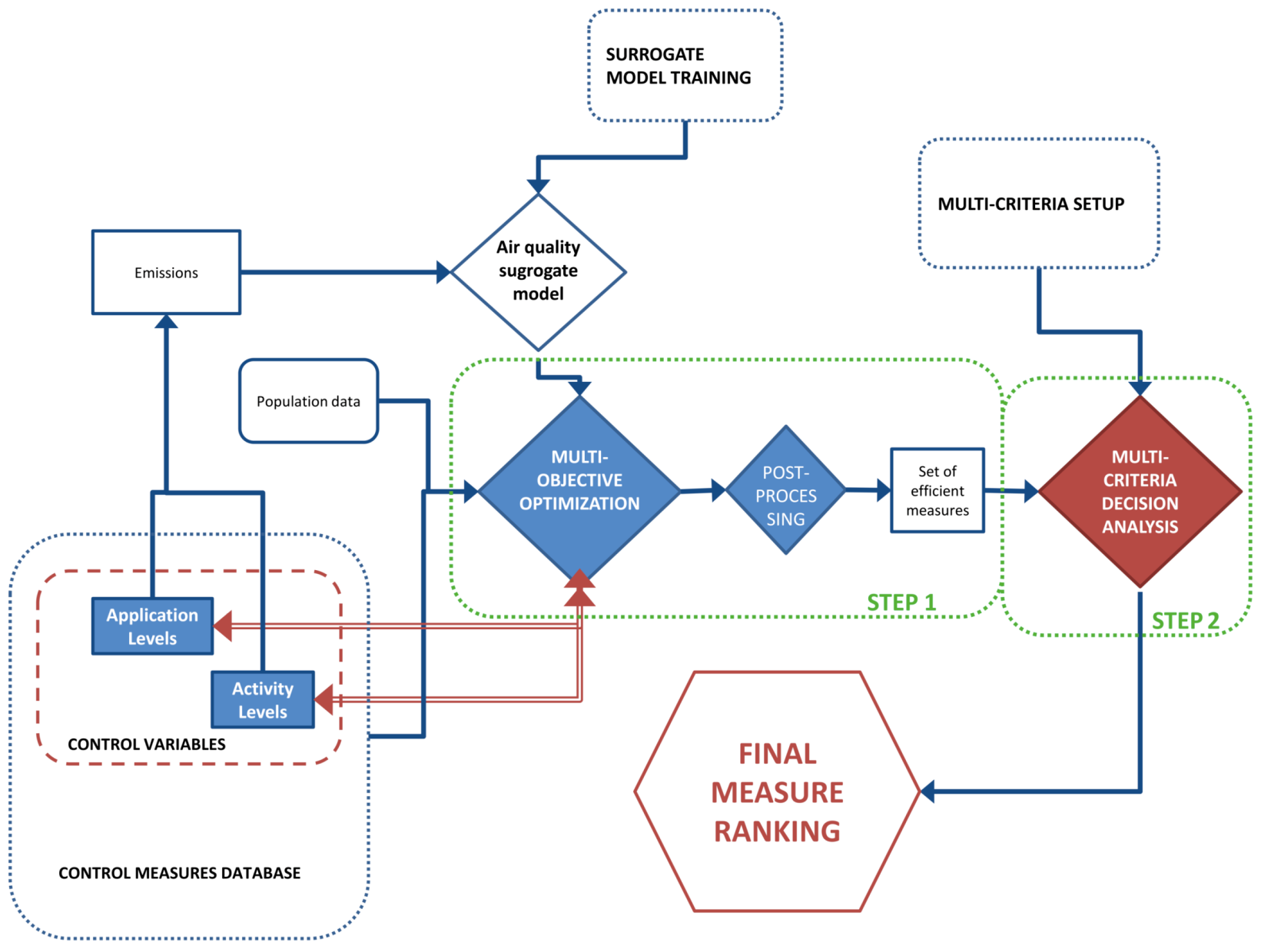
5.3. Multi-Objective Model Setup

In the first step, since multiphase deterministic 3D modelling systems ([29,30]) cannot be used to compute pollutant concentrations and air quality indexes, due to the required computational cost and the number of simulations needed to solve a multi-objective problem, they have been substituted by statistical surrogate models, identified processing the results of a set of Chemical Transport Models simulations ([31,32,33]). In particular, following the methodologies presented in [34,35,
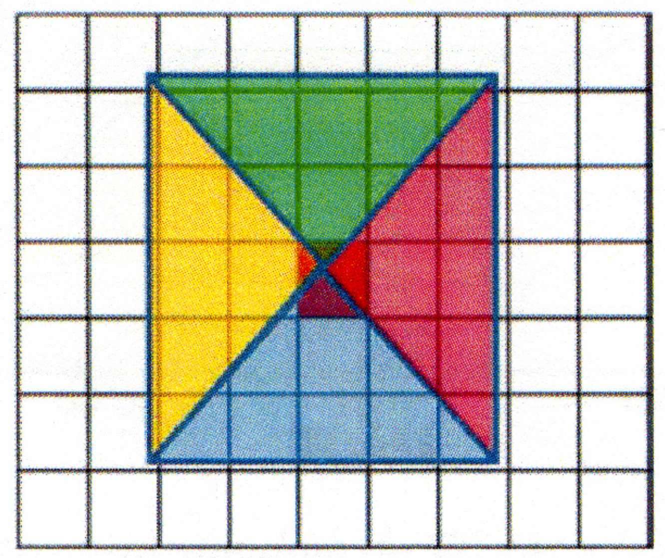
36], models based on Artificial Neural Networks (ANNs), have been applied, mainly due to their features of low computational requirements, good performances and ability to reproduce non-linear functions. According to the same studies, three important features must be selected to identify a model that is adequate to the domain under study: radius of influence, input shape, and training data design. The first feature should be chosen considering that AQI values in a cell depend on precursor emissions generated in distant cells. While the second one allows to consider the dominant winds of the domain (mainly East-West and North-South in the current domain). Reference [35] presented a technique allowing to consider both this aspect by summing the emissions of cells belonging to triangular slices around a target cell for which the model should be able to compute the AQI. An example of this scheme can be seen in Appendix BFigure A1. Before the training of the models, also the extension of these slices (radius of influence) must be chosen so that it is appropriate for the AQI and the considered domain. To select the best radius of influence, different ANN models are identified by varying the radiuses. The radius choice falls on the ANN model showing the highest correlation and lowest mean squared error with respect to deterministic model simulations. The features of the Artificial Neural Network applied in the current work are summarized in Table 1.
The set of scenarios needed to properly tune the surrogate model, has to be simulated by means of a deterministic model and should have the highest data variability in the input-output space (highest information content) and cover the possible emission variations of the P M 10 precursors, but at the same time, the number of scenarios considered should be limited, due to the computational time required by the deterministic model. When applied in the Multi-objective problem, the surrogate model should reproduce scenarios in which the emissions of each precursor can vary between a maximum value, which corresponds to the maximum projected emissions for a chosen reference or “basecase” year, and a minimum value, representing the Maximum Feasible Reduction (MFR).
For this purpose two dummy extreme scenarios (HIGH and LOW scenario) can be defined by combining the maximum and the minimum values obtained from other 4 scenarios derived from the application of INEMAR 2008 emission inventory [37] rescaled to 2010 and projection parameters derived from GAINS Italy database [3].
Between the two extremes, a small number of emission scenarios are created by applying a Sobol sequences based algorithm [38] in order to evenly distribute precursors emission values between the higher and lower possible values.
InAppendix BTable A2 the precursor reduction factors derived from the algorithm are presented for each of the 14 emission scenarios that will be simulated and used for the surrogate model training.
These scenarios have been simulated by means of TCAM (Transport Chemical Aerosol Model), a three-dimensional Eulerian model [39], in order to obtain the corresponding concentration scenarios needed for the training phase. These data are then divided into 2 smaller sets: one is the identification dataset used for the model training, containing 4/5 of the total data and the validation dataset, containing the remaining 1/5, used to evaluate the performances of the model. To perform this separation, all the training scenarios have been concatenated and 1 tuple every five has been extracted from the identification dataset and stored in the validation dataset.
Table 2 presents correlation (corr) and normalized root mean squared error (nrmse) for the validation dataset comparing TCAM target outputs and the ANN outputs. The first line refers to a comparison of the resulting concentrations, the second line shows the same indexes but computed on the concentration reductions with respect to the HIGH scenario in order to remove the effect of the background concentrations from the evaluation. High values of correlation (corr) and a low normalized root mean squared error (nrmse) attest the fitness of the model.

5.4. Results

In the first part of this section, Step 1 results are shown and discussed. The objective of this stage is to find a small set of effective measures to be included in Step 2 and, also, to quantitatively evaluate through the system the performance that these measures have for some of the criteria that will be evaluated in the MCDA. The set of measures that has been evaluated through this first phase is composed of 288 end-of-pipe measures, 42 energy measures and 13 switch measures.
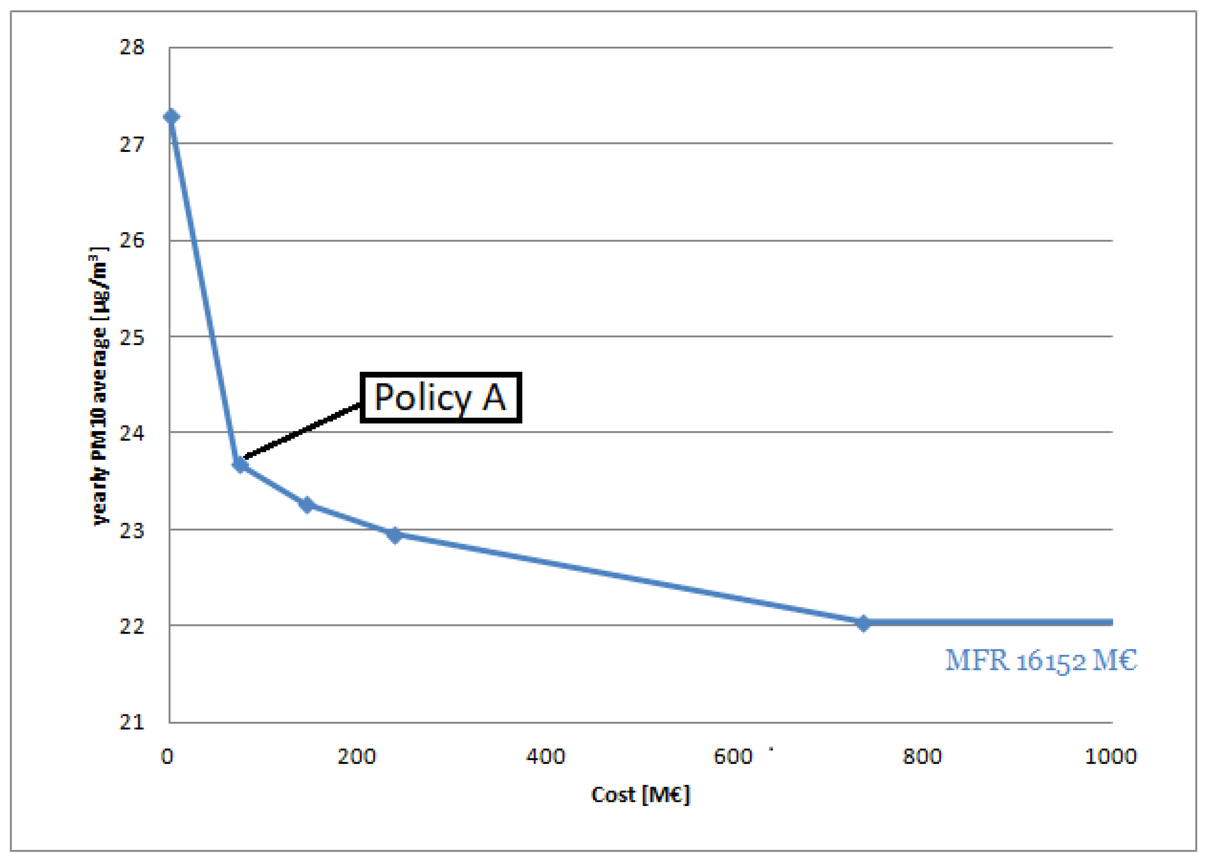
In Figure 3, the Pareto front is shown, representing the solutions of the multi-objective problems in terms of cost and yearly average P M 10 concentrations. The starting scenario at the extreme left is the Current Legislation scenario expected for 2020, while the point on extreme right is the maximum feasible reduction obtainable with the considered measures while optimizing only the Air Quality objective. Due to the extremely high costs of some energy measures, the MFR has a cost of 16,152 M and a yearly average P M 10 concentration of 21.92 μ g/m 3 . This means that, by applying the policy identified by the the second point of the curve (72 M, 23.7 μ g/m 3 ), P M 10 yearly average concentrations can be reduced of 67% with respect to the MFR at only the 0.3% of its cost.
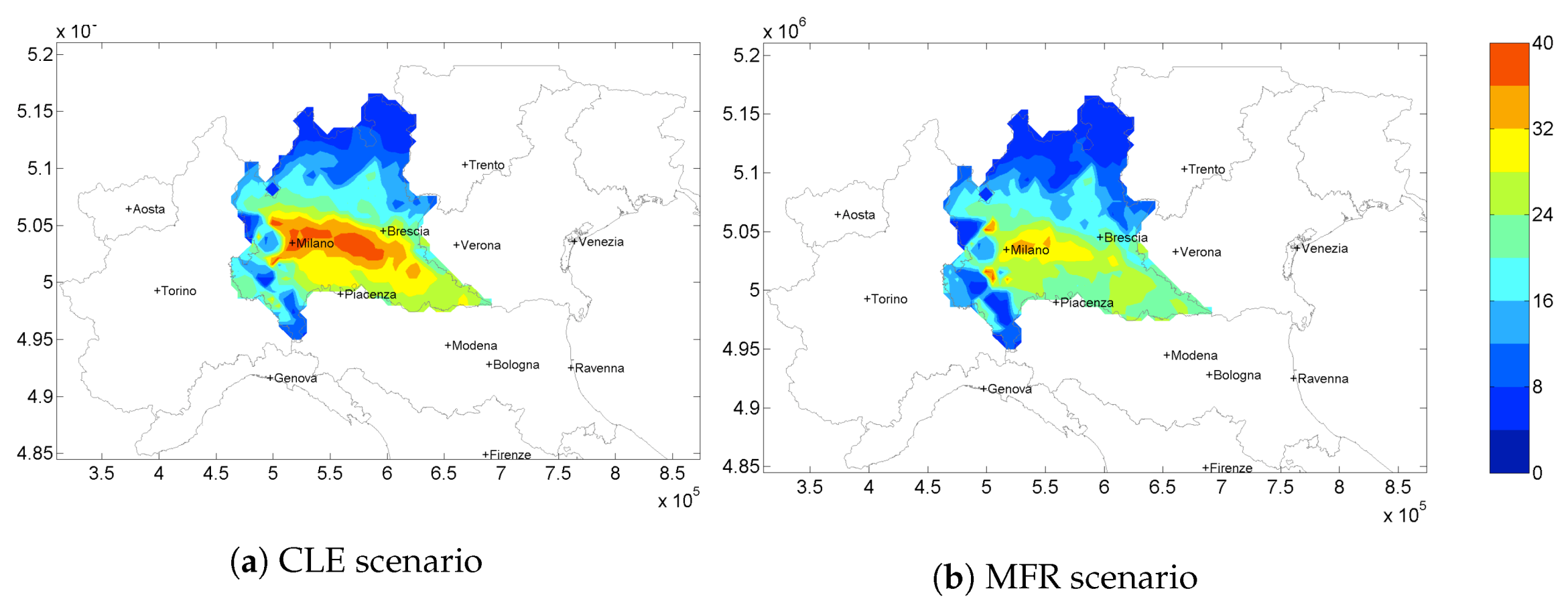
In Figure 4 the P M 10 yearly average concentration maps for CLE 2020 scenario (Figure 4a) and the Maximum Feasible Reduction obtainable (Figure 4b) are shown.
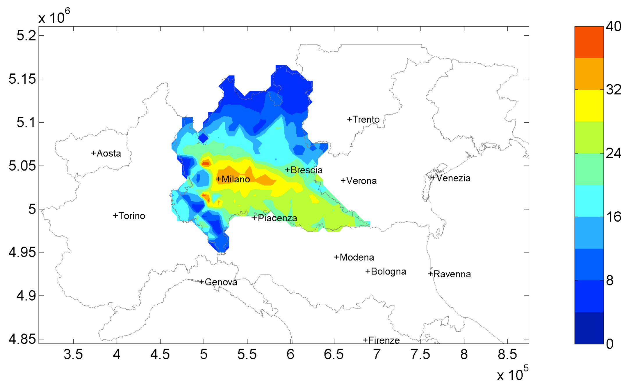
The same air quality index is shown in Figure 5 for the solution at a 72 M/year cost (Policy A). This solution is one of the closest solution to the maximum curvature of the Pareto front. This means that a cost increase, with respect to this point, results only in a small decrease of P M 10 concentrations. The comparison between this last map with the maximum reduction obtainable (Figure 4b), highlights that yearly P M 10 concentrations are not so different, except for small differences in the central part of the domain. So, adopting an effective solution such as Policy A, high amounts of P M 10 can be reduced over the domain at a low cost.
The yearly P M 10 concentrations obtained from Policy A show the effect of the combined application of nearly 100 measures whose application rates undergo an increase with respect to CLE scenario (starting point for the optimization). So, given also the impact of the non-linearities, it is not possible to define a-priori the set of measures with the highest impact on the AQI. The selected measures are the 10 measures with the highest Δ Θ for energy and both end-of-pipe measures. In Appendix CTable A3 the measures selected to undergo Step 2 are shown with their relative Δ Θ values. Only 4 of the 13 energy measures are present in the table. The reason is that these measures are usually expensive, so, for a relatively low cost policy such as Policy A, only 4 of these are cheap enough to produce relevant effects on the air quality if little money is invested in them.
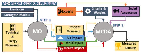
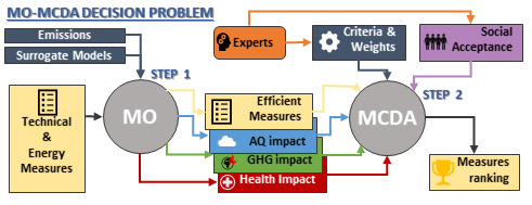
Once the measures have been selected, the MCDA can be applied, considering four criteria:
  • c1: social acceptance;
  • c2: implementation cost;
  • c3: health impact, in terms of YOLL due to long-term P M 10 exposure;
  • c4: effect on GHGs emissions, considering C O 2 equivalents.
All these criteria have scores ranged from 0 to 10 with an ascending direction of preference for all the criteria. This means that if a measure is the cheapest, it has the maximum score (10) in the cost criterion. Criterion c1, as well as the weighting factors for all the criteria, have been evaluated though a questionnaire submitted to a pool of experts. Instead, for the last three criteria (c2, c3 and c4), since it is possible to obtain reliable quantitative information by solving the multi-objective optimization, the scores attributed to each measure have been computed by applying the MOA individually to the selected measures. The values used for criteria c2, c3 and c4, are respectively computed through Equations (3), (6) and (5). These data have then been normalized between 0 and 10 and the results are shown in Table A4.
Appendix DTable A4 summarizes the performance coefficients and criteria weights chosen by the experts’ (performance matrix).
Preference thresholds are associated with the total number of alternatives to efficiently discriminate among the options, providing a smoothed “relative distance” between the alternatives. In order to achieve this, indifference and preference thresholds are computed for the different criteria (shown in Appendix DTable A5) with the use of Equations (8) and (9). Fixed thresholds were applied and veto thresholds were not considered. The methodological approach continues with the application of the LAMSADE ELECTRE III-IV package [40] applying an outranking relation based on decision maker’s preferences and providing two partial pre-orders of alternatives: an ascending and a descending one.
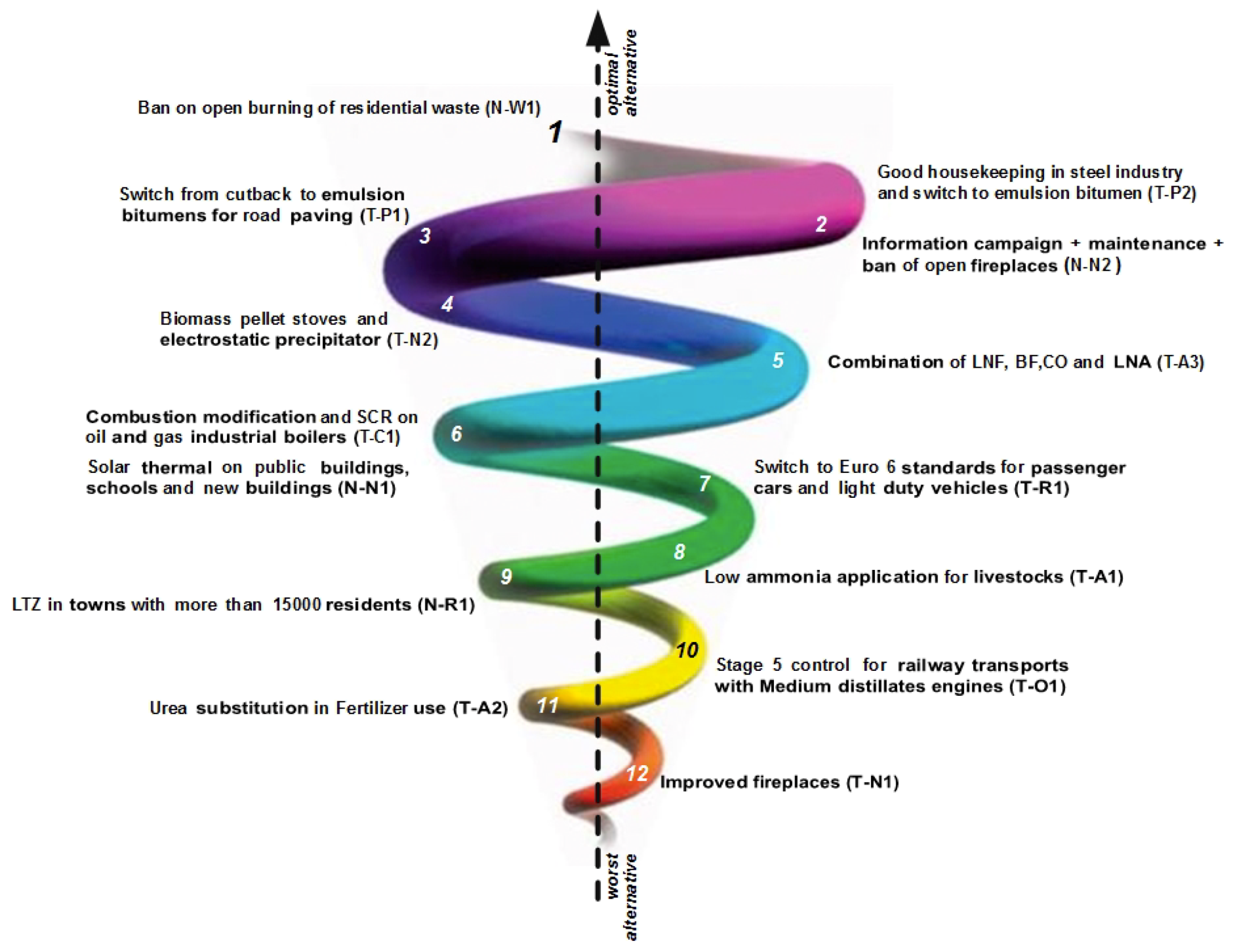
The merge of these two pre-orders is used to compute the final ranking of all alternatives, shown in Figure 6. This figure presents the Median Pre-order, that is a complete pre-order and it is built in the following way: the alternatives are classified through an intersection of the distillations results and two incomparable alternatives in the same position are classified according to the differences in their positions in the two distillations. The first letter in the code identifies if a measure is end-of-pipe (T) or a fuel consumption measure (N).
The first measures in this ranking are: (1) “Ban on open burning of residential waste”, (2) “Good housekeeping in steel industry and switch to emulsion bitumen”, (3) “Information campaign + maintenance + ban of open fireplaces”. “Ban on open burning of residential waste” has high scores in the first two criteria, this means that it is considered socially acceptable and has a low cost. The health impact and effect on GHG emission scores are low but the experts assigned the lowest weights to these criteria. This is true also for measure T-P2, while the third measure has lower values in c1 and c2, but higher scores for health impact and effect on GHG emissions. It is possible to see that, despite the fact that only 4 energy measures were considered, two out of the three best measures are energy ones. The other two ranked 6th (N-N1) and 9th (N-R1) because of an extremely high cost (the first) and low scores in all the criteria except the cost (the second).
The multi criteria decision analysis approach is strongly dependent from the choice of the criteria to be considered and the experts’ views on criteria weights. In Table 3, an example of the final measure ranking is shown, if the decision makers decide to ignore one of the criteria. The central column represent the ranking considering all the criteria, the left column shows the rank changes when leaving out the effect on GHG emissions, while the last one on the right presents the ranking when leaving out the effect on health. It can be seen that, due to the fact that the criteria removed are the ones with the lowest weight, even if there are small changes, the measures in the first places are the same, despite few position changes. The same happens for the last positions. This dependence on subjective choices stresses the need of a consider a shared choice of the criteria among the people involved in the decision process and a wide pool of stakeholders to evaluate the measure scores for the different criteria when modelling data are not available.

6. Conclusions

Long-term exposure to particulate matter can be a well known potential threat to human health, mainly in currently industrialized parts of the world. Air quality policy makers are tasked with developing sound plans to reduce population exposure to these pollutants. Such plans consist in a set of measures able to effectively reduce pollutant concentrations on a domain, by acting on precursor emissions. These abatement strategies should be defined on the basis of integrated assessment techniques able to support the decision makers in the selection of efficient emission reduction measures and to assess their impacts for different dimensions (e.g., GHG, health, costs).
This research is focused on the development of an integrated assessment methodology merging multi-objective optimization (MOA) and multi criteria decision analysis (MCDA), allowing to include in the decision process technological, health, social and economic aspects.
The objective of the work is the formulation of a two-steps decision-making problem where the first step allows to identify a small set of efficient measures though the solution of a multi-objective problem, evaluating policy costs, air quality indexes, health impacts and GHG emissions; through the second step, that is an application of a MCDA, it is possible to compute a final ranking for the measures including also social criteria.
The proposed methodology has been tested on a case study over Lombardy region, (a domain located in Northern Italy) to control the impact of particulate matter ( P M 10 ) exposure on population health. The analysis of the MOA solutions (Step 1) allows to identify effective emission reduction measures, supporting Environmental Authorities in the choice of policies to reduce the health impact of particulate matter with a minimum economic cost. The results underline that, to effectively reduce particulate matter exposure in Lombardy region, it is not possible to focus in abating emissions on a single activity macro-sector, but it is necessary to act simultaneously in different ones. The set of efficient measures, selected solving the MOA, has been subsequently considered for the application of an MCDA (Step 2) to provide a final measure ranking due to the aggregation of social acceptance (evaluated by experts) of abatement measures as well as costs, effectiveness on health impact and GHGs emission reduction (evaluated through the application of Step 1). The final ranking shows that the proposed approach is an easily applicable method for the inclusion of subjective criteria such as the social acceptance in the decision problem, as well as for the reduction of the impact that discording experts opinion can have on the solution. Despite the fact that experts are still needed to evaluate the weights of the criteria and the social aspects, Step 1 helps to remove the human factor from the choice of the efficient measures to be tested and provides reliable quantitative data to evaluate their performances.

Author Contributions

Conceptualization, E.T. and M.V.; Formal analysis, E.T.; Methodology, E.T., C.V. and M.V.; Software, E.T.; Supervision, M.V.; Writing—original draft, E.T.; Writing—review & editing, E.T., C.V. and M.V.

Funding

This research received no external funding.

Acknowledgments

The authors would like to thank Giorgio Guariso (Politecnico di Milano, IT) and Michela Maione (Università di Urbino, IT) for their expertise and valuable co-operation during the work.

Conflicts of Interest

The authors declare no conflict of interest.

Abbreviations

The following abbreviations are used in this manuscript:
GHGGreenhouse gases
PMParticulate matter
VOCVolatile organic compounds
MOAMulti-objective approach
MCDAMulti criteria decision analysis
ANNMulti-objective approach
CLECurrent legislation scenario
MFRMaximum feasible reduction

Appendix A

Table A1. The 11 main CORINAIR categories.
SNAP CodeCategory Description
1Combustion in energy and transformation industries
2Non-industrial combustion plants
3Combustion in manufacturing industry
4Production processes
5Extraction and distribution of fossil fuels/geothermal energy
6Solvent and other product use
7Road transport
8Other mobile sources and machinery
9Waste treatment and disposal
10Agriculture and forestry, land use and wood stock change
11Nature

Appendix B

Figure A1. Schematic representation of the input configuration.
Atmosphere 10 00381 g0a1
Table A2. Emission reduction coefficients for the different scenarios and the 5 considered P M 10 precursors.
ScenarioNO x VOCSO 2 NH 3 PM10
111111
200000
301111
410111
511011
611101
711110
80.250.250.250.750.25
90.250.750.250.750.25
100.250.750.750.750.25
110.50.50.50.50.5
120.750.250.750.750.25
130.750.750.250.750.25
140.250.250.750.250.75
Scenario 1 and 2 of Table A2 represents respectively the HIGH and LOW emission scenarios. Single precursor reductions are represented in the scenarios from 3 to 7 and the last 7 scenarios consider the combined reduction of all the pollutants.These reductions must be applied to the emission interval that can actually be reduced ( H I G H L O W ) in order to compute the emissions.

Appendix C

Table A3. Final measures chosen to undergo the second Step of the methodology with the final Δ Θ values for Policy A.
MacrosectorCodeMeasure Δ Θ
TECHNICAL MEASURESAgricultureT-A1Low ammonia application for livestocks82%
T-A2Urea substitution in Fertilizer use100%
T-A3Combination of LNF, BF, CO and LNA43%
Combustion in manufacturing industryT-C1Combustion modification and SCR on oil and gas industrial boilers67%
Non industrial combustion plantsT-N1Improved fireplaces68%
T-N2Biomass pellet stoves and electrostatic precipitator10%
Other mobile sources and machineryT-O1Stage 5 control for railway transports with Medium distillates engines33%
Production processesT-P1Switch from cutback to emulsion bitumens for road paving23%
T-P2Good housekeeping in steel industry and switch to emulsion bitumen47%
Road transportT-R1Switch to Euro 6 standards for passenger cars and light duty vehicles30%
ENERGYMEASURESNon industrial combustion plantsN-N1Solar thermal on public buildings, schools and new buildings9%
N-N2Information campaign + maintenance + ban of open fireplaces33%
Road transportN-R1LTZ in towns with more than 15,000 residents2%
Waste treatment and disposalN-W1Ban on open burning of residential waste31%

Appendix D

Table A4, summarizes the performance coefficients and weights chosen by the experts’ (performance matrix), as well as the measure scores for c2, c3 and c4, defined applying the optimization results. Observing this table it is clear that, considering the effects of the measures on GHGs emission reduction, energy measures (reducing the fuel consumption) can have higher impacts. The impact on GHGs of measure N-N1 is in fact extremely high.
Table A4. Performance matrix containing the scores for each abatement measure in the four different criteria considered. (EXP) and (MOA) indicate which criteria have been evaluated respectively by experts or through multi-objective approach.
CodeMeasureSocial AcceptanceCostHealth ImpactEffect on GHG
(expert)(MOA)(MOA)(MOA)
TECHNICAL MEASUREST-A1Low ammonia application for livestocks6.09.82.30.1
T-A2Urea substitution in Fertilizer use6.09.03.60.1
T-A3Combination of LNF, BF, CO and LNA7.04.410.00.1
T-C1Combustion modification and SCR on oil and gas industrial boilers7.010.00.20.1
T-N1Improved fireplaces6.51.16.70.1
T-N2Biomass pellet stoves and electrostatic precipitator7.09.16.71.0
T-O1Stage 5 control for railway transports with Medium distillates engines6.59.90.30.1
T-P1Switch from cutback to emulsion bitumens for road paving8.510.00.10.1
T-P2Good housekeeping in steel industry and switch to emulsion bitumen7.510.00.11.0
T-R1Switch to Euro 6 standards for passenger cars and light duty vehicles6.09.16.70.1
ENERGYMEASURESN-N1Solar thermal on public buildings, schools and new buildings8.51.02.610.0
N-N2Information campaign + maintenance + ban of open fireplaces9.07.47.02.0
N-R1LTZ in towns with more than 15000 residents5.510.00.11.0
N-W1Ban on open burning of residential waste9.09.90.50.1
WEIGHT OF THE CRITERION0.30.40.20.1
Table A5. Preference and indifference thresholds.
c1c2c3c4
Preference0.0900.2310.2560.254
Indifference0.0270.0690.0770.076

References

  1. Künzli, N.; Laura, P.; Regula, R. Air Quality and Health; European Respiratory Society: Lausanne, Switzerland, 2010. [Google Scholar]
  2. Seaton, A.; Godden, D.; MacNee, W.; Donaldson, K. Particulate air pollution and acute health effects. Lancet 1995, 345, 176–178. [Google Scholar] [CrossRef]
  3. Amann, M.; Bertok, I.; Borken-Kleefeld, J.; Cofala, J.; Heyes, C.; Höglund-Isaksson, L.; Klimont, Z.; Nguyen, B.; Posch, M.; Rafaj, P.; et al. Cost-effective control of air quality and greenhouse gases in Europe: Modeling and policy applications. Environ. Model. Softw. 2011, 26, 1489–1501. [Google Scholar] [CrossRef]
  4. Rotaris, L.; Danielis, R.; Marcucci, E.; Massiani, J. The urban road pricing scheme to curb pollution in Milan, Italy: Description, impacts and preliminary cost–benefit analysis assessment. Transp. Res. Part A Policy Pract. 2010, 44, 359–375. [Google Scholar] [CrossRef]
  5. Pisoni, E.; Volta, M. Modeling Pareto efficient {PM10} control policies in Northern Italy to reduce health effects. Atmos. Environ. 2009, 43, 3243–3248. [Google Scholar] [CrossRef]
  6. Carnevale, C.; Douros, J.; Finzi, G.; Graff, A.; Guariso, G.; Nahorski, Z.; Pisoni, E.; Ponche, J.L.; Real, E.; Turrini, E.; et al. Uncertainty evaluation in air quality planning decisions: a case study for Northern Italy. Environ. Sci. Policy 2016, 65, 39–47. [Google Scholar] [CrossRef]
  7. Carnevale, C.; Finzi, G.; Pisoni, E.; Volta, M.; Wagner, F. Defining a nonlinear control problem to reduce particulate matter population exposure. Atmos. Environ. 2012, 55, 410–416. [Google Scholar] [CrossRef]
  8. Cecchel, S.; Chindamo, D.; Turrini, E.; Carnevale, C.; Cornacchia, G.; Gadola, M.; Panvini, A.; Volta, M.; Ferrario, D.; Golimbioschi, R. Impact of reduced mass of light commercial vehicles on fuel consumption, CO2 emissions, air quality, and socio-economic costs. Sci. Total Environ. 2018, 613–614, 409–417. [Google Scholar] [CrossRef] [PubMed]
  9. Vlachokostas, C.; Achillas, C.; Moussiopoulos, N.; Banias, G. Multicriteria methodological approach to manage urban air pollution. Atmos. Environ. 2011, 45, 4160–4169. [Google Scholar] [CrossRef]
  10. Achillas, C.; Vlachokostas, C.; Moussiopoulos, N.; Banias, G. Prioritize strategies to confront environmental deterioration in urban areas: Multicriteria assessment of public opinion and experts’ views. Cities 2011, 28, 414–423. [Google Scholar] [CrossRef]
  11. Ambrasaite, I.; Barfod, M.B.; Salling, K.B. MCDA and Risk Analysis in Transport Infrastructure Appraisals: The Rail Baltica Case. Procedia Soc. Behav. Sci. 2011, 20, 944–953. [Google Scholar] [CrossRef]
  12. Theodor, J.S.; Durbach, I. Dealing with Uncertainties in MCDA. In Multiple Criteria Decision Analysis; Greco, S., Ehrgott, M., Figueira, J., Eds.; International Series in Operations Research & Management Science; Springer: New York, NY, USA, 2016; Chapter 12; pp. 467–496. [Google Scholar] [Green Version]
  13. Chalabi, Z.; Milojevic, A.; Doherty, R.M.; Stevenson, D.S.; MacKenzie, I.A.; Milner, J.; Vieno, M.; Williams, M.; Wilkinson, P. Applying air pollution modelling within a multi-criteria decision analysis framework to evaluate UK air quality policies. Atmos. Environ. 2017, 167, 466–475. [Google Scholar] [CrossRef]
  14. Blond, N.; Carnevale, C.; Douros, J.; Finzi, G.; Guariso, G.; Janssen, S.; Maffeis, G.; Martilli, A.; Pisoni, E.; Real, E.; et al. A framework for integrated assessment modelling. Springer Briefs Appl. Sci. Technol. 2017, 9–35. [Google Scholar] [CrossRef]
  15. EUR. Guidance for the development of National Air Pollution Control Programmes under Directive (EU) 2016/2284 of the European Parliament and of the Council on the reduction of national emissions of certain atmospheric pollutants. Off. J. Eur. Union C 77 2019, 1–33. Available online: https://eur-lex.europa.eu/legal-content/EN/TXT/?uri=uriserv:OJ.C_.2019.077.01.0001.01.ENG (accessed on 9 July 2019).
  16. Turrini, E.; Carnevale, C.; Finzi, G.; Volta, M. A non-linear optimization programming model for air quality planning including co-benefits for GHG emissions. Sci. Total Environ. 2018, 621, 980–989. [Google Scholar] [CrossRef] [PubMed]
  17. Carnevale, C.; Pisoni, E.; Volta, M. A multi-objective nonlinear optimization approach to designing effective air quality control policies. Automatica 2008, 44, 1632–1641. [Google Scholar] [CrossRef]
  18. Castelletti, A.; Galelli, S.; Ratto, M.; Soncini-Sessa, R.; Young, P. A general framework for Dynamic Emulation Modelling in environmental problems. Environ. Model. Softw. 2012, 34, 5–18. [Google Scholar] [CrossRef]
  19. Carnevale, C.; Finzi, G.; Pisoni, E.; Volta, M. Neuro-fuzzy and neural network systems for air quality control. Atmos. Environ. 2009, 43, 4811–4821. [Google Scholar] [CrossRef]
  20. Bickel, P.; Friedrich, R. ExternE: Externalities of Energy, Methodology 2005 Update; Technical Report; IER, University of Stuttgart: Stuttgart, Germany, 2005. [Google Scholar]
  21. Maystre, L.; Pictet, J.; Simos, J. Méthodes Multicritères ELECTRE. Description, Conseils Pratiques et Cas d’Application à la Gestion Environnementale; Presses Polytechniques et Universitaires Romandes: Lausanne, Switzerland, 1994. [Google Scholar]
  22. Roy, B.; Bouyssiou, D. Aide Multicritere a la Decision: Methods et Cas.; Economica: Paris, France, 1993. [Google Scholar]
  23. Rogers, M.; Bruen, M. Choosing realistic values of indifference, preference and veto thresholds for use with environmental criteria within {ELECTRE}. Eur. J. Oper. Res. 1998, 107, 542–551. [Google Scholar] [CrossRef]
  24. Haralambopoulos, D.; Polatidis, H. Renewable energy projects: structuring a multi-criteria group decision-making framework. Renew. Energy 2003, 28, 961–973. [Google Scholar] [CrossRef]
  25. Achillas, C.; Vlachokostas, C.; Moussiopoulos, N.; Banias, G. Decision support system for the optimal location of electrical and electronic waste treatment plants: A case study in Greece. Waste Manag. 2010, 30, 870–879. [Google Scholar] [CrossRef]
  26. Aardenne, J.V.; Tooly, L.; Rypdal, K.; Pulles, T. Good Practice for Clrtap Emission Inventories; Technical Report; EMEP/EEA: Copenhagen, Denmark, 2004. [Google Scholar]
  27. IIASA. GAINS Europe Online. Available online: http://gains.iiasa.ac.at/gains/EUN/index.login (accessed on 2 July 2018).
  28. Lombardia, R. Piano Regionale degli Interventi per la Qualità dell’Aria (PRIA). 2013. Available online: http://www.regione.lombardia.it/wps/portal/istituzionale/HP/DettaglioRedazionale/istituzione /direzioni-generali/direzione-generale-ambiente-energia-e-sviluppo-sostenibile/piano-regionale -interventi-qualita-aria-pria/piano-regionale-interventi-qualita-aria-pria (accessed on 17 July 2018).
  29. Sokhi, R.; José, R.S.; Kitwiroon, N.; Fragkou, E.; Pérez, J.; Middleton, D. Prediction of ozone levels in London using the MM5–CMAQ modelling system. Environ. Model. Softw. 2006, 21, 566–576. [Google Scholar] [CrossRef]
  30. Cuvelier, C.; Thunis, P.; Vautard, R.; Amann, M.; Bessagnet, B.; Bedogni, M.; Berkowicz, R.; Brandt, J.; Brocheton, F.; Builtjes, P.; et al. CityDelta: A model intercomparison study to explore the impact of emission reductions in European cities in 2010. Atmos. Environ. 2007, 41, 189–207. [Google Scholar] [CrossRef]
  31. Friedrich, R.; Reis, S. Tropospheric Ozone Abatement; Springer: Berlin/Heidelberg, Germany, 2000. [Google Scholar]
  32. Ryoke, M.; Nakamori, Y.; Heyes, C.; Makowski, M.; Schöpp, W. A simplified ozone model based on fuzzy rules generation. Eur. J. Oper. Res. 2000, 122, 440–451. [Google Scholar] [CrossRef] [Green Version]
  33. Carnevale, C.; Finzi, G.; Pederzoli, A.; Turrini, E.; Volta, M. Lazy Learning based surrogate models for air quality planning. Environ. Model. Softw. 2016, 83, 47–57. [Google Scholar] [CrossRef]
  34. Corani, G. Air quality prediction in Milan: feed-forward neural networks, pruned neural networks and lazy learning. Ecol. Model. 2005, 185, 513–529. [Google Scholar] [CrossRef] [Green Version]
  35. Carnevale, C.; Finzi, G.; Guariso, G.; Pisoni, E.; Volta, M. Surrogate models to compute optimal air quality planning policies at a regional scale. Environ. Model. Softw. 2012, 34, 44–50. [Google Scholar] [CrossRef]
  36. Pisoni, E.; Carnevale, C.; Volta, M. Multi-criteria analysis for PM10 planning. Atmos. Environ. 2008, 30, 1–10. [Google Scholar] [CrossRef]
  37. ARPA Lombardia. INEMAR—Lombardy Region Emission Inventory. 2011. Available online: http://www.inemar.eu/xwiki/bin/view/InemarDatiWeb/Emissionunderlinetag|Inventory (accessed on 21 January 2016).
  38. Sobol, I. Uniformly distributed sequences with an addition uniform property. USSR Comput. Math. Math. Phys. 1976, 16, 236–242. [Google Scholar] [CrossRef]
  39. Carnevale, C.; Finzi, G.; Pisoni, E.; Volta, M. Modelling assessment of PM10 exposure control policies in Northern Italy. Environ. Model. Softw. 2008, 217, 219–229. [Google Scholar] [CrossRef]
  40. Vallée, D.; Zielniewicz, P. Electre III/IV Version 3.x: Aspects Méthodologiques; Document du Lamsade n∘85; Université Paris-Dauphine: Paris, France, 1994. [Google Scholar]
Figure 1. Scheme of the decisional problem formalization.
Atmosphere 10 00381 g001
Figure 2. The domain considered in the case study.
Atmosphere 10 00381 g002
Figure 3. Pareto curve presenting the solutions of the Step 1 (MOA).
Atmosphere 10 00381 g003
Figure 4. Maps of the P M 10 yearly average concentrations in [ μ g/m 3 ] for the current legislation scenario (a) (optimization base-case) and the MFR scenario (b).
Atmosphere 10 00381 g004
Figure 5. Maps of the yearly P M 10 average concentrations in [ μ g/m 3 ] for Policy A scenario.
Atmosphere 10 00381 g005
Figure 6. Final measure ranking as resulting from the application of Step 2.
Atmosphere 10 00381 g006
Table 1. Architecture of the Artificial Neural Network applied to reproduce yearly P M 10 concentrations.
NETLayersHidden Layer NeuronsActivation FunctionOutput FunctionRadius of Influence [Km]
PM10 yearly mean220Log- sigmoidHyperbolic tangent sigmoid24
Table 2. Correlation (corr) and normalized root mean squared error (nrmse) resulting from the validation of the ANN model applied in the current work to reproduce P M 10 yearly concentrations.
CORRNRMSE
Concentrations0.990.15
Variation of concentrations0.90.44
Table 3. Comparison between three solutions of a MCDA if different criteria are chosen.
RankC1 + C2 + C3C1 + C2 + C3 + C4C1 + C2 + C4
1N-W1N-W1N-W1
2T-N2T-P2T-P2
3N-N2N-N2T-P1
4T-P1T-P1T-N2
5T-A3T-N2T-C1
6T-P2T-A3N-N2
7T-A1T-C1T-O1
8T-R1N-N1N-N1
9T-C1T-R1T-A1
10T-O1T-A1N-R1
11N-N1N-R1T-A3
12T-A2T-O1T-A2
13T-N1T-A2T-R1
14N-R1T-N1T-N1

