Article

Grapevine Phenology of cv. Touriga Franca and Touriga Nacional in the Douro Wine Region: Modelling and Climate Change Projections

1
Centre for the Research and Technology of Agro-Environmental and Biological Sciences, CITAB, Universidade de Trás-os-Montes e Alto Douro, UTAD, 5000-801 Vila Real, Portugal
2
INRA, US1116 AgroClim, 84914 Avignon, France
3
ADVID, Associação para o Desenvolvimento da Viticultura Duriense, Parque de Ciência e Tecnologia de Vila Real–Régia Douro Park, 5000-033 Vila Real, Portugal
*
Author to whom correspondence should be addressed.
Agronomy 2019, 9(4), 210; https://doi.org/10.3390/agronomy9040210
Submission received: 3 April 2019 / Revised: 17 April 2019 / Accepted: 23 April 2019 / Published: 25 April 2019
(This article belongs to the Special Issue Viticulture and Winemaking under Climate Change)

Abstract

:
Projections of grapevine phenophases under future climate change scenarios are strategic decision support tools for viticulturists and wine producers. Several phenological models are tested for budburst, flowering, and veraison and for two main grapevine varieties (cv. Touriga Franca and Touriga Nacional) growing in the Douro Demarcated Region. Four forcing models (Growing degree-days, Richardson, Sigmoid, and Wang) and three dormancy models (Bidabe, Smoothed Utah and Chuine), with different parameterizations and combinations, are used. New datasets, combing phenology with weather station data, widespread over the Douro wine region, were used for this purpose. The eight best performing models and parameterizations were selected for each phenophase and variety, based on performance metrics. For both cultivars, results revealed moderate performances (0.4 < R2 < 0.7) for budburst, while high performances (R2 > 0.7) were found for flowering and veraison, particularly when Growing degree-days or Sigmoid models are used, respectively. Climate change projections were based on a two-member climate model ensemble from the EURO-CORDEX project under RCP4.5. Projections depicted an anticipation of phenophase timings by 6, 8 or 10–12 days until the end of the century for budburst, flowering, and veraison, respectively. The inter-model variability is of approximately 2–4 days for flowering and veraison and 4–6 days for budburst. These results establish grounds for the implementation of a decision support system for monitoring and short-term prediction of grapevine phenology, thus promoting a more efficient viticulture.

1. Introduction

Viticulture is one of the most important socioeconomic sectors in Portugal. From a global perspective, Portugal is currently the 11th-largest wine producer and the 9th wine exporter in the world [1]. Portugal accounts for approximately 194,000 ha of vineyard area and with a wine production around 6.7 × 10⁶ hL [1]. Almost half of this production is exported, accounting for nearly 2% of national export income [2]. The country is divided into 14 viticultural regions (12 in the mainland and 2 in the islands), with 25 Denominations of Origin (DOs). Douro/Porto, Vinhos-Verdes, Alentejo, and Lisboa are the main regions in terms of wine production. Although the Alentejo wine region is the most productive [3], the Douro/Porto wine region has the largest vineyard area and is the main region in terms of production, accounting for ca. 25% of all wine produced in Portugal [2].
The Douro/Porto wine region, also known as Douro Demarcated Region (DDR), has unique features, where vineyards are traditionally grown on terraces over steep slopes along the mountainous Douro valley and in an almost monocultural system, resulting in a UNESCO (United Nations Educational, Scientific and Cultural Organization) human heritage vineyard landscape. A large number of grapevine varieties (Vitis vinifera L.) are grown in the region, being many of them native. The complex physiographic and pedoclimatic characteristics of the DDR not only provide a wide range of terroirs for grapevine growth [4], but also make wine production very costly in terms of labour force and vineyard management [5]. Given the heterogeneous conditions in which grapevines are grown within the DDR, it is imperative to better understand the climatic influences on grapevine development in order to improve vineyard management in such a diverse region. In effect, monitoring the phenological phases and timings are some of the most useful information for planning the necessary viticultural practices in each developmental stage. This knowledge may promote more adjusted cultural practices, eventually optimizing production and quality at harvest.
It is known that grapevine development and growth are mainly driven by meteorological and climatic factors [6]. Therefore, factors such as temperature, solar radiation and precipitation may have a great influence on phenology, yields, and grape berry quality and attributes [7,8]. In particular, temperature is a fundamental factor in controlling grapevine phenological development and ripening [9,10,11,12,13]. Phenology models have been developed for a wide range of species, including grapevines, and using observational data from many different countries and regions [14]. Several previous studies have been performed in order to model the main phenological stages of grapevines, e.g., enabling a classification of varieties for technical proposes [15], to predict phenophases or to assess the impact of climate change on phenology [16].
Many different models have been developed during the last 60 years to simulate grapevine phenology. The modelling of budbreak was explored by several authors assuming different hypothesis [17,18,19,20,21,22]: taking or not into account the dormancy period, interactions between dormancy and post-dormancy periods, starting at a fixed date (e.g., January 1st, February 15th, March 15th). These models were tested for many different varieties under different climatic conditions. For flowering and veraison, the conventional linear growing degree-days model (GDD) was initially proposed by Amerine and Winkler [23]. This simple temperature accumulation model uses daily mean temperatures, with a fixed base temperature of 10 °C, and onsets temperature accumulation at April 1st. Others models have been calibrated and tested to simulate flowering and veraison, such as the linear model proposed by Duchene, et al. [24], with a formulation similar to the Winkler model, and the curvilinear model of Wang and Engel, later adapted by García de Cortázar-Atauri, et al. [25]. The latter model was improved by incorporating an optimal temperature (25 to 30 °C) and an upper critical threshold temperature (40 °C). The GFV model (Grapevine Flowering and Veraison model) was proposed by Parker, et al. [26] and Parker, et al. [27]. This model is similar to GDD, but with a 0 °C base temperature and starting temperature accumulation on March 1st. This last model was developed to classify different grapevine varieties within them. Finally, Molitor, et al. [28] developed a high-resolution model to simulate all the phenological stages described in the BBCH (Biologische Bundesanstalt, Bundessortenamt und CHemische Industrie) scale using a capped model. As such, the performance of several phenology models should be tested at a regional level, as there is no best model for all varieties and conditions.
Phenological models may also be coupled with climate change scenarios to project the potential impacts of future climates on phenological timings and grapevine development [21,24,25,29,30,31,32,33]. Projected increases in temperature are expected to drive earlier development stages and, as a result, a general advancement of grapevine phenology [24,34,35,36,37]. Those changes will affect the ripening period, commonly occurring in the warmest part of summer, and may lead to aromas and acidity losses [38]. Consequently, currently planted varieties, which are grown under quite specific conditions today, may no longer thrive in the same place under modified environmental conditions in the future [39]. Therefore, it is critical to understand to what extent temperature may influence the timings of the reproductive and vegetative cycles, as well as identifying varietal differences in phenology and maturity [26]. While several studies have assessed the phenological timings in many regions worldwide, a comprehensive study of phenology in the DDR was not undertaken so far, due to the overall lack of phenological and meteorological data. Hence, the present study attempts to overcome this drawback, by presenting the first grapevine phenological study for the DDR.
Along the previous lines, the aims of the present study are twofold: 1) to identify suitable phenological models for three main phenological timings (budburst, flowering, and veraison) of two leading grapevine varieties (cv. Touriga Franca and cv. Touriga Nacional) currently grown in the DDR; 2) to assess the climate change impacts on these phenological timings and varieties. The datasets and methodologies are described in Section 2. The results are presented in Section 3. Section 4 will provide a discussion and a summary of the main conclusions.

2. Materials and Methods

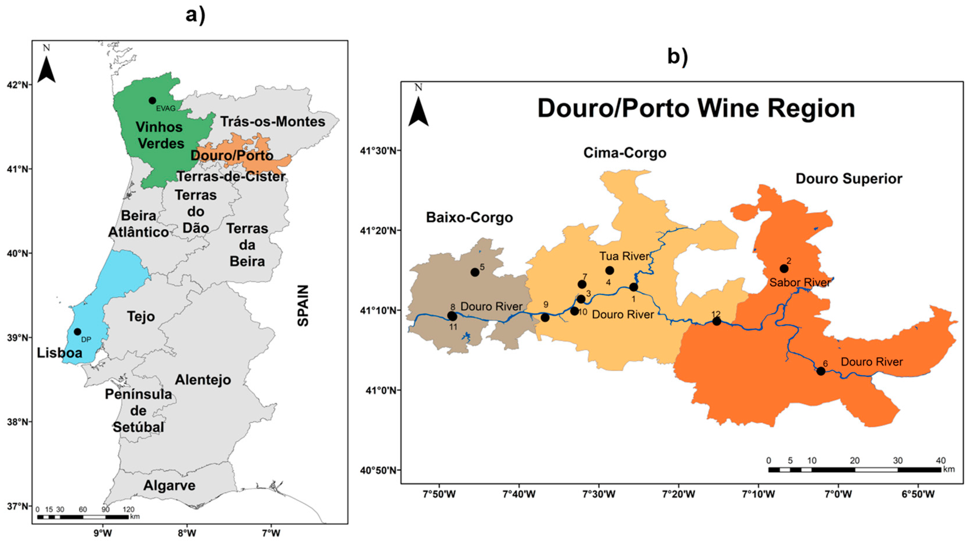
2.1. Study Area and Datasets

The present study targets the Douro/Porto Wine Region (DDR), located in Northern Portugal (Figure 1a). The DDR is characterized by Mediterranean-type climates, with typically dry and warm summers, though a wide range of mesoclimates and microclimates do exist throughout the region, mostly driven by the multifaceted orography and distance to the North Atlantic. Important east–west gradients in both temperatures and precipitation can be found within the region, and are typified by its 3 sub-regions: from Baixo-Corgo (westernmost sector) to Cima-Corgo (middle sector) and to Douro Superior (easternmost sector) (Figure 1b). This spatial variability is further enhanced by important differences in soil properties, though soils are mostly originated from schist bedrocks [40].
In the present study, phenological data recorded at 12 vineyards (“Quintas”) in the DDR, with data available over the period 2014–2017 (4 years), were used (Figure 1b). The phenological timings were recorded through observations based on the BBCH scale adapted to grapevines and when at least 50% of a pre-defined set of homogenous plants reach the corresponding stage. Budburst (BBCH 07), flowering (BBCH 65) and veraison (BBCH 81) were considered herein [41]. Data for two main grapevines varieties grown in Portugal were selected: cv. Touriga Franca (TF) and cv. Touriga Nacional (TN). As information for other varieties (cv. Tempranillo, cv. Tinta Amarela and cv. Moscatel-Galego) was indeed very limited and inconsistent among vineyards, they were not taken into consideration. Furthermore, in order to enhance the statistical robustness of the selected models for a given grapevine variety, the phenological timings for the same variety for all sites (and terroirs) were considered for model calibration.
Owing to the relatively small sample size of the DDR dataset for model calibration (12 sites × 4 years = 48 records), the same phenological timings for TF and TN from two other Portuguese wine regions were also used: Lisboa (central-west) and Vinhos Verdes (north-west) (Figure 1a). Phenological records were available for the following locations (Table 1): “Dois Portos—DP” (Lisboa Wine Region), with 20 years of data within the full period of 1990–2014, and “Estação Vitivinícola Amândio Galhano—EVAG” (Vinhos Verdes Wine Region), with records over the period of 2005–2009 (5 years). Therefore, the total sample size is extended to 73 records for each phenological timing and variety, thus enabling a higher statistical robustness in model calibration. A summary of the entire phenology dataset is provided in Table 1.
For the DDR, daily mean temperature records from the meteorological stations installed at the different vineyard sites and over the period of 2014–2017 (4 years) were used (Figure 1b). For the other two wine regions (Vinhos Verdes-EVAG and Lisboa-DP), the local temperature time series were estimated from the nearest-point of a very-high resolution (~1 km) gridded daily temperature dataset for Portugal [42]. Phenology and temperature data for the Douro Wine Region were provided by the “Associação para o Desenvolvimento da Viticultura Duriense—ADVID”, after collecting information among their members, while phenology data for Lisboa-DP and Vinhos Verdes-EVAG were provided by the “Instituto Nacional de Investigação Agrária e Veterinária”, INIAV, and by EVAG, respectively.

2.2. Phenological Models

Phenological models were selected based on previous studies, which have already shown moderate-to-high performance in simulating grapevine phenological timings in other regions [19,26,43]. Two main groups of phenological models were used: chilling models (Bidabe, Chuine, and Smoothed Utah), used to simulate the dormancy phase; and the forcing models (GDD, Richardson, Sigmoid, and Wang) applied to simulate thermal accumulation during the three phenophases: budburst, flowering, and veraison (Table 2).
In the case of budburst, two approaches were tested: sequential models that allow integrating a dormancy phase (described using chilling models) and models without dormancy period (starting at a fixed date—January 1st—and only using forcing models). For sequential models, dormancy was herein calculated starting from August 1st of the previous year, as proposed by García de Cortázar-Atauri, Brisson and Gaudillere [19]. For flowering and veraison only the forcing models were applied. Table 2 describes the tested models and their relevant bibliographic references, while Table 3 describes their corresponding mathematical formulations and tested parameters.
For all these models, the parameters were fixed at specific thresholds, some of them defined in the literature taking into account previous research: Tm = 0 °C, TM = 40 °C and Topt = 25–26 °C for Wang, Tlow = 5 °C and Thigh = 20–25 °C for Richardson, and Tb = 0 °C for GDD [19,20,26,43]. Besides these default models, the freely-adjusted best-fit parameters for each of these four models were also selected in the present study, as their performances can be significantly better than using the default parameters. The best eight performing models for each phenological phase were selected based on the performance metrics explained below. The models were considered for each of the three phenophases: dormancy to budburst (D-B), budburst to flowering (B-F), and flowering to veraison (F-V). The calibration of different models was performed independently for each phenophase and for the two selected grapevines varieties (TF and TN).

2.3. Modelling Tools and Performance Verification

In this study, the Phenological Modelling Platform, PMP [14], was used to test and calibrate different phenological models applied to grapevines. PMP is an intuitive platform that allows users to apply and test different phenological models for several purposes. In this platform, climatic and phenological data were used in order to calibrate the models, i.e., estimate the best-fit model parameters, for a specific location and a pre-defined time period. PMP estimates best-fit parameters following an iterative optimization procedure, based on the simulated annealing algorithm of Metropolis, et al. [51].
For each specific location, the input data used were daily mean (Td), maximum (Tmax) and minimum (Tmin) temperatures, latitude and observed phenological timings for budburst, flowering, and veraison (in days of the year, DOY). The model performance is assessed herein by four commonly used metrics: the determination coefficient (R2), root-mean-square error (RMSE), Nash–Sutcliffe coefficient of efficiency (EF) and the Akaike Information Criterion (AIC). Their definitions are as follows:
R M S E   =   i   =   1 n ( O i   P i ) 2 n   ,
E F   =   1   i   =   1 n ( O i   P i ) 2 i   =   1 n ( O i   O ¯ i ) 2   ,
A I C   =   n × ln ( i   =   1 n ( O i   P i ) 2 n )   + 2 k + ( 2 k ( k + 1 ) n k 1 )
where O i represents the observed phenological dates, O ¯ i represents the average observed value, P i represents simulated phenological dates, n is the sample size, and k is the number of parameters.
EF varies between –∞ and +1, +1 corresponds to a perfect fit, 0 corresponds to the performance of the null model (average), while a negative value corresponds to a worse prediction than the null model. The A I C takes into account the number of model parameters, with the lowest value corresponding to a model that represents the highest variance ratio in the observed dataset with the fewest parameters (parsimony principle). Further, in order to take into consideration model overfitting, a leave-one-out cross-validation scheme was applied to every simulation, following the same methodology as described by Chuine, et al. [52], and the RMSE metric was accordingly adapted to Root Mean Square Error of Prediction (RMSEP), defined as:
R M S E P   =   i   =   1 n ( O i P i ^ ) 2 n
where P i ^ is the predicted value obtained from a leave-one-out cross-validation approach [53].

2.4. Future Climate Projections

PMP also allows running simulations using climatic data generated from different anthropogenic forcing scenarios and climate model experiments, applying the previously calibrated phenology models. For the simulations under future climates, the daily temperature time series generated by a two-member ensemble of climate model chains (Table 4), produced within the framework of the EURO-CORDEX (Coordinated Downscaling Experiment—European Domain) project, were used [54]. A distribution-based scaling method was applied as a bias correction method by EURO-CORDEX [55]. The nearest-point time series for each vineyard site was extracted from the original grid (~12 km spacing). Data for the future period of 2020–2100, under the Representative Concentration Pathway 4.5 (RCP4.5), was selected. This scenario corresponds to an intermediate/moderate anthropogenic (greenhouse gas) forcing and corresponds to an increase of the global mean temperature slightly above 2 °C, thus marginally fulfilling the Paris Agreements.
Although the model calibration was undertaken using data from three wine regions, which enabled an improvement of the statistical robustness of the model fits, the future projections were only developed for the Douro wine region, as this study was never carried out previously. The outputs for the eight selected phenology models and for each phenological phase were applied to each climate model output, thus obtaining 12 sites × 3 phases × 8 phenology models × 2 climate models (576 simulations). In the future simulations, the D-B phase started at August 1st (with dormancy) or January 1st (without dormancy, Sigmoid model), as previously described. As in the observational period, for the other two phenophases (B-F and F-V) the starting date was set at the previous phenological stage (budburst or flowering), but now using the average time series of simulated budburst or flowering dates by the corresponding eight phenology models.

3. Results

3.1. Model Performance Verification

As previously mentioned, the sample size of the observed phenology dataset used for model calibration is of 73 records for each phenological timing and variety. For TF, the minimum/mean/maximum DOY is 61/77/98 for budburst (from March 2nd to April 8th), 112/138/158 for flowering (from April 22nd to June 7th) and 177/201/222 for veraison (from June 26th to August 10th). For TN, the observed minimum/mean/maximum DOY is 64/78/100 (from March 5th to April 10th) for budburst, 112/140/158 for flowering (from April 22nd to June 7th) and 170/213/235 for veraison (from June 19th to August 23rd). Despite the large spread in the dates of each phenophase, these results show that phenophase timings are commonly earlier for TF than for TN, particularly for veraison. In addition, the correlation coefficients between the time series for DP and EVAG, in their overlapping period (2005–2009), are very high (>0.80), thus showing a strong coherency in the inter-annual variability of the phenophase timings, despite the regional differences. No correlations can be computed with the DDR, as only 2014 overlaps with DP.
The best eight models for each corresponding phenophase are shown in Table 5; Table 6 for TF and TN, respectively. For the D-B phenophase, seven sequential models and one forcing model were chosen. The results show that for D-B, the RMSEP is of 6–7 days for TF, while it reaches values of almost 8 days for TN (Table 5 and Table 6). The EF varies from 0.35 to 0.41 (TF) or from 0.15 to 0.23 (TN). The corresponding coefficients of determination (R2) show values ranging from 0.54 to 0.64 (TF) or from 0.41 to 0.48 (TN). It is important to highlight that most of the models chosen present different sets of parameters, showing very different temperature responses. As the sample size of observed data does not allow choosing a specific model with high statistical confidence, it is important to maintain this diversity in order to cover a wide range of possibilities. Further, there is no clear difference between the experiments with or without dormancy simulation. In fact, the use of a sequential model does not seem to improve over the single-model even if the number of model parameters is higher in the sequential-model [19]. The AIC values hint at this conclusion, revealing higher values in the sequential models compared to the Sigmoid model. Overall, the model performances for D-B are thus moderate and the best performances are obtained from the Sigmoid model, for both TF and TN, or, alternatively, from the Bidabe + Wang (TF) or Bidabe + GDD (TN) sequential models.
In the case of B-F (Table 5 and Table 6), the RMSEP is of 5–6 days (TF and TN), i.e., less one day than for the D-B phase. The EF also presents much higher values than in the previous phenophase, between 0.60 to 0.70 in TF and from 0.61 to 0.69 in TN. The R2 are also significantly higher, varying from 0.78 to 0.87 (0.78 to 0.84) in TF (TN). The AIC values are within the range 159–172 (170–180) in TF (TN). Among the three phenophases, the best results are achieved for F-V (Table 5 and Table 6), with RMSEP of 4–5 days in TF and 5–6 days in TN. The EF varies from 0.76 to 0.84 in TF and from 0.83 to 0.86 in TN. The AIC shows relatively low values, from 141 to 158, in TF, and from 151 to 165, in TN.
The errors between simulated and observed dates for TF, over the period from 1995 to 2017, show relatively high values for D-B (up to ca. 20 days), while they are mostly lower than 10 days for B-F and F-V (Figure 2). As expected, the errors are much more scattered for D-B than for the other two phenophases, with an error compensation between the periods of 1998–2003 and 2005–2009. There is also some non-stationarity in errors, which may be attributed to non-homogeneities in phenophase and/or climate data. Similar considerations can be made for TN (Figure S1).

3.2. Future Projections

The simulated temperatures from the ensemble of two climate models under RCP4.5 were performed for 8 phenological models and for 12 vineyard sites in the DDR. In order to avoid an excessively large number of figures, only the mean curves over the 12 sites in the DDR are presented in Figure 3; Figure 4. The corresponding panels for each climate model chain are presented separately in Figures S2–S5. Apart from minor differences, site-specific figures are very similar (not shown). For all models, a gradual anticipation of the three main phenological phases (downward long-term trends) is clear for both TF (Figure 3) and TN (Figure 4), despite not being linear and revealing noteworthy fluctuations. Analysing the chronograms for both TF and TN, it is evident that the eight selected models for each phenophase render coherent results (low inter-model ranges), mostly for flowering and veraison. In general, the inter-model range is of nearly 4–6 days for budburst and 2–4 days for flowering and veraison. The correlations between D-B phase and January–April mean temperature, between B-F phase and May–June mean temperature and between F-V phase and July–August mean temperature are clear, thus highlighting that the projected changes are largely driven by changes in mean temperatures over specific time periods. However, some differences between the curves of temperature and mean phenophase timings are found. This can be explained by the fact that the temperature curves correspond to multi-month averages, while the phenological timings are determined by 1) the accumulation of daily temperatures over longer time periods and 2) by the preceding phenophase timings. Furthermore, apart from GDD, model responses are non-linear functions of temperature.
In the case of D-B for TF, a mean anticipation of 6 days is expected from 2020 to 2100, with important inter-decadal variability, without a clear trend until 2070, followed by a more pronounced long-term decrease from 2070 to 2100 (Figure 3a). The Smoothed-Wang and the Smoothed-Sigmoid are the closest models to the mean. For B-F in TF, a clear anticipation is expected after 2040, despite the delay in the period of 2060–2070 (Figure 3b), which can be attributed to a cooler period in the future climate (Figure 3b). Overall, a mean anticipation of 8 days in flowering is projected until 2100. The Sigmoid (d = −0.2, e = 16.9) and the Wang (Tm = 0 °C, TM = 40 °C, Topt = 29.1 °C) models show the closest correspondence with the mean. For F-V, an anticipation of 8–10 days over the full period is projected (Figure 3c), with analogous temporal variability to B-F (Figure 3b). The Richardson (Tlow = 0 °C, Thigh = 21.5 °C) and the Wang (Tm = 0 °C, TM = 40 °C, Topt = 26 °C) models are very close to the mean.
Similar considerations can be made for TN (Figure 4). For D-B of TN, the Smoothed-GDD and Smoothed-Wang are the closest to the mean. For B-F of TN, the Richardson (Tlow = 7 °C, Thigh = 20.8 °C) and the Sigmoid (d = −0.3, e = 14.4) models show the most central behaviour. For F-V of TN, the Richardson (Tlow = 0 °C, Thigh = 23.7 °C) and the Wang (Tm = 0 °C, TM = 40 °C, Topt = 26.9 °C) models are the closest to the mean. In addition, the anticipation of veraison for TN is more pronounced than for TF (8 to 12 days). These anticipations in phenological timings are in clear agreement with other studies worldwide [21,32,34]. These shifts towards earlier timings may result in changes to the currently established cultural practices and potentially affect the wine characteristics of the Douro.

3.3. Inter-Model Spread

Regarding the inter-model variability, some differences can be highlighted. For D-B of TF (Figure 3a), all the selected models show very similar results, with the exception of the sequential models Bidabe-Richardson and Smoothed-GDD, which reveal some significant departures from the model average. These two models simulate systematically earlier budburst timings than the other models (Figure 3a), despite their strong agreement, as expected taking into account that their transfer functions are very similar (Table 5). Further, the Sigmoid, Bidabe-Sigmoid, Smoothed-Sigmoid, and Chuine-Sigmoid models are in close agreement, as the second model is the same, also suggesting that dormancy does not play a key role in the final outcome. Similarly, the Bidabe-Wang and Smoothed-Wang also reveal similar behaviour throughout the future period. For B-F of TF (Figure 3b), the GDD (Tb = 0 °C) model shows a tendency to have later timings. Conversely, the Wang (Tm = 0 °C, TM = 31.6 °C, Topt = 25.5 °C) model reveal earlier timings throughout the analysed period. For F-V of TF (Figure 3c), the selected models highlight a very strong coherency, apart from some light discrepancies found for GDD (Tb = 0 °C), with earlier timings.
For D-B in TN (Figure 4a), the Bidabe-Wang presents the earliest phenological timings throughout the study time period. For B-F in TN (Figure 4b), the GDD (Tb = 0 °C) model presents later phenological timings, while the Wang (Tm = 0 °C, TM = 26.5 °C, Topt = 21.8 °C) model shows earlier phenological timings along all the study period. The other models show very strong agreement between them and with values closer to the mean. However, it should be stated that models showing higher agreement are not necessarily more realistic in reproducing timings under future conditions. Lastly, regarding F-V in TN (Figure 4c), the Wang (Tm = 0 °C, TM = 40 °C, Topt = 25 °C) shows the later timings, while the GDD (Tb = 0 °C) shows the earlier timings.

4. Discussion and Conclusions

Phenological models are a key tool for viticulturists, as they provide valuable information for management and planning in vineyards [7]. The accurate prediction phenological timings promotes best practices and the timely implementation of suitable measures to optimize grapevine yields and grape berry quality [56,57,58,59]. Moreover, future projections of potential changes in the phenological timings may also deliver important information for medium-to-long term planning [60]. Despite the aforementioned high economic value of the DDR, no previous studies were conducted for this region on phenological modelling and simulation. Unique datasets, combining phenological timings with weather station records, in the Douro wine region were used herein. The weather stations used were installed at the vineyard locations, which is of utmost importance for a proper phenological modelling [61]. Furthermore, two of the most important grapevine varieties cultivated in the Douro wine region (TF and TN) were selected (cv. Touriga Franca—TF and cv. Touriga Nacional—TN). Despite the relatively large number of sites in the Douro valley (12 Quintas), data is only available over a maximum period of 4 years. This dataset was thereby complemented with data from two other Portuguese wine regions (Lisboa and Vinhos Verdes) and for the same grapevine varieties (TF and TN). This approach led to more robust results, as the sample sizes for model calibration were significantly enlarged.
It was herein demonstrated that some specific phenological models are particularly suitable to the simulation of the two selected grapevine varieties. For all phenophases, specific parameter values were chosen within each model (e.g., Tb in GDD), either by selecting reference values, recommended from previous studies, or best-fit values. Although the recommended values did not always lead to the best performances in our study, no definite conclusions can be withdrawn, as only two varieties were selected herein and the corresponding sample sizes are relatively low. As a whole, the present study allowed the identification of the best phenological models (a set of eight models per phenophase), thus warranting their application both in an operational mode (real-time monitoring and short-term prediction) and in future climate change projections (long-term prediction). Nevertheless, more data will allow improving the selection of the best model and the accuracy of the predictions.
In general terms, the results highlight that the phenological models are better in simulating flowering or veraison than budburst. This may be due to the fact that dormancy and other relevant physiological processes are not sufficiently understood, but might be important drivers of budburst occurrence. As also described by García de Cortázar-Atauri, Brisson and Gaudillere [19], no clear improvements were found concerning the incorporation of a dormancy period in the model structure. Moreover, the model performances are generally higher for TF than for TN, which may suggest that the latter is slightly less sensitive to thermal forcing, though this needs to be properly addressed by further research, including field experiments. Overall, the Bidabe-Wang and Sigmoid models showed the best results for budburst in TF, while the Bidabe-GDD and Sigmoid models present the highest performances in TN. For flowering, in both grapevine varieties (TF and TN), the very simple GDD model, with a base temperature of ca. 7 °C, revealed the best performances. Lastly, the Sigmoid model provided the best performances for veraison in both varieties. Hence, the GDD linear model is not always the best approach to model and simulate grapevine phenology, as the phenology–temperature relationship may be of non-linear nature. The present study results are comparable, in terms of model performance, to other studies in other winemaking regions worldwide [19,26,27,43,62,63,64,65]. Although the aforementioned models provide the best approaches, it is important to bear in mind that they are bound to this particular phenology dataset.
Climate change projections of the phenophase timings, based on a two-member ensemble of state-of-the-art climate model chains, hinted at anticipations of the phenophase timings up to 10–12 days until the end of the twentieth first century, though with some dissimilarities amongst phenophases and varieties. In addition, there is a strong coherency between phenological models, as the results do not change significantly with the model choice, apart from a few exceptions, thus highlighting the robustness of the projections. Nonetheless, different grapevines varieties exhibit greater phenological sensitivity to temperature changes than others, which limits the extrapolation of the results found herein to other locations and varieties. These projections for the Douro are in agreement with observed trends worldwide, such as for Alsace (France), [Jones [66]] for the California (USA) and Bock, et al. [67] for Franconia (Germany). These shifts towards earlier phenophase onsets can potentially result in changes to the currently established wine characteristics and typicity. In effect, the expected warming may result in unbalanced wines, with high alcoholic content and excessively low acidity and altered colour and aroma [68,69]. These impacts can be partially overcome through the adoption of suitable adaptation measures, such as selection of grapevine varieties that tend to produce berries with lower sugar contents and higher acidity levels in warm climates. Suitable selections of variety-clone-rootstock combinations are among the most effective medium-to-long term measures to cope with climate change. The cultivation of late maturation cultivars is also key to mitigate the anticipation of phenological stages in the vineyards. Short term measures, like irrigation, application of sun screens, changes in training systems, soil management and mulching application, may also be envisioned by producers and winemakers.
The present study aims at providing some initial insights that can be of use not only to future research, but also to regional stakeholders. In the near future, it is expected that the outcomes of this study will be implemented on a web platform, maintained by ADVID, which will deliver information on phenological timings to regional wine companies and grounded on a network of operational weather stations. Future research should also envision the improvement of the current models, such as by extending the phenological datasets with new data from other regions in Portugal or in other countries where the selected varieties also grow. Other grapevine varieties may also be considered in future studies, but there is a critical lack of information for them, particularly on the Douro native/autochthonous varieties, which may considerably hamper their simulation.

Supplementary Materials

The following are available online at https://www.mdpi.com/2073-4395/9/4/210/s1, Figure S1: Chronograms of the departures between simulated and observed phenological timings of each phenophase on cv. Touriga Nacional: (a) Dormancy–Budburst (D-B); (b) Budburst–Flowering (B-F), and (c) Flowering–Veraison (F-V), obtained from the eight selected models (cf. legends) and assembled for the 14 vineyard sites (Figure 1). Figure S2. Chronograms (2020–2100, RCP4.5) of the phenological timings (days of the year, DOY) of (a) Dormancy–Budburst (D-B); (b) Budburst–Flowering (B-F); and (c) Flowering–Veraison (F-V), and for cv. Touriga Franca (TF), obtained from the eight selected models (cf. legends), averaged for the 12 sites in the DDR (Figure 1) and for the climate model CNRM-SHMI. The average maximum-minimum ranges for each phenophase (among the different phenology models) are also pointed out by vertical arrows. Figure S3. Chronograms (2020–2100, RCP4.5) of the phenological timings (days of the year, DOY) of (a) Dormancy–Budburst (D-B); (b) Budburst–Flowering (B-F); and (c) Flowering–Veraison (F-V), and for cv. Touriga Nacional (TN), obtained from the eight selected models (cf. legends), averaged for the 12 sites in the DDR (Figure 1) and for the climate model CNRM-SHMI. The average maximum-minimum ranges for each phenophase (among the different phenology models) are also pointed out by vertical arrows. Figure S4. As for Figure S2, but for the climate model MPI-CLM. Figure S5. As for Figure S3, but for the climate model MPI-CLM.

Author Contributions

Conceptualization, H.F., I.G.d.C.-A., and J.A.S.; Data curation, R.C., A.F., M.C.V., C.C., and S.R.; Formal analysis, R.C., H.F., and S.R.; Funding acquisition, J.A.S.; Investigation, R.C., H.F., A.F., M.C.V., C.C., S.R., and J.A.S.; Methodology, R.C., A.F., I.G.d.C.-A., and J.A.S.; Project administration, J.A.S.; Resources, A.F., I.G.d.C.-A., and J.A.S.; Software, R.C., H.F., A.F., I.G.d.C.-A., and S.R.; Supervision, H.F., I.G.d.C.-A., and J.A.S.; Validation, I.G.d.C.-A.; Visualization, S.R.; Writing—original draft, R.C.; Writing—review and editing, H.F., A.F., I.G.d.C.-A., M.C.V., C.C., S.R., and J.A.S.

Funding

This research and the APC were funded by the European Union’s Horizon 2020 Research and Innovation Programme, grant number 810176.

Acknowledgments

This study was supported by the Clim4Vitis project—“Climate change impact mitigation for European viticulture: knowledge transfer for an integrated approach”, funded by European Union’s Horizon 2020 Research and Innovation Programme, under grant agreement nº 810176. This work was also supported by National Funds by FCT—Portuguese Foundation for Science and Technology, under the project UID/AGR/04033/2019. FCT scholarship SFRH/BPD/119461/2016 and contract CEECIND/00447/2017 are acknowledged. The authors also acknowledge the FCT scholarship given to R.C., PD/BD/135326/2017, under the Doctoral Programme ‘Agricultural Production Chains—from fork to farm’ (PD/00122/2012). Climate data was provided by ADVID, SOGRAPE vinhos SA, Quinta do Noval, and Direcção Regional de Agricultura e Pescas do Norte (DRAPN). Phenological data from DDR was obtained through the support of ADVID members.

Conflicts of Interest

The authors declare no conflict of interest.

References

  1. OIV. State of the Vitiviniculture World Market; OIV: Paris, France, 2018; p. 14. [Google Scholar]
  2. IVV. Vinhos e Aguardentes de Portugal, Anuário 2017; Ministério da Agricultura, do Desenvolvimento Rural e das Pescas, Instituto da Vinha e do Vinho: Lisboa, Portugal, 2017; p. 224.
  3. Fraga, H.; Santos, J.A. Vineyard mulching as a climate change adaptation measure: Future simulations for Alentejo, Portugal. Agric. Syst. 2018, 164, 107–115. [Google Scholar] [CrossRef]
  4. Fraga, H.; Costa, R.; Santos, J.A. Multivariate clustering of viticultural terroirs in the douro winemaking region. Cienc. Tec. Vitivinic. 2017, 32, 142–153. [Google Scholar] [CrossRef]
  5. Fraga, H.; Santos, J.A. Daily prediction of seasonal grapevine production in the Douro wine region based on favourable meteorological conditions. Austr. J. Grape Wine Res. 2017, 23, 296–304. [Google Scholar] [CrossRef]
  6. Keller, M. Phenology and growth cycle. In The Science of Grapevines, 2nd ed.; Keller, M., Ed.; Academic Press: San Diego, CA, USA, 2015; Chapter 2; pp. 59–99. [Google Scholar] [CrossRef]
  7. Moriondo, M.; Ferrise, R.; Trombi, G.; Brilli, L.; Dibari, C.; Bindi, M. Modelling olive trees and grapevines in a changing climate. Environ. Model. Softw. 2015, 72, 387–401. [Google Scholar] [CrossRef]
  8. Andreoli, V.; Cassardo, C.; La Iacona, T.; Spanna, F. Description and preliminary simulations with the Italian vineyard integrated numerical model for estimating physiological values (IVINE). Agronomy 2019, 9, 94. [Google Scholar] [CrossRef]
  9. Winkler, A.J. General Viticulture; University of California Press: Berkly, CA, USA, 1974. [Google Scholar]
  10. Huglin, P. Nouveau Mode D’évaluation des Possibilités Héliothermiques d’un Milieu Viticole. COMPTES RENDUS de L’académie D’AGRICULTURE; Académie d’agriculture de France: Paris, France, 1978. [Google Scholar]
  11. Jones, G.V.; Davis, R.E. Climate influences on grapevine phenology, grape composition, and wine production and quality for Bordeaux, France. Am. J. Enol. Viticult. 2000, 51, 249–261. [Google Scholar]
  12. Jones, G.V.; Duchêne, E.; Tomasi, D.; Yuste, J.; Braslavska, O.; Schultz, H.R.; Martinez, C.; Boso, S.; Langellier, F.; Perruchot, C.; et al. Changes in European winegrape phenology and relationships with climate. In Proceedings of the XIV GESCO Symposium, Geisenheim, Germany, 23–26 August 2005. [Google Scholar]
  13. Van Leeuwen, C.; Garnier, C.; Agut, C.; Baculat, B.; Barbeau, G.; Besnard, E.; Bois, B.; Boursiquot, J.-M.; Chuine, I.; Dessup, T.; et al. Heat requirements for grapevine varieties is essential information to adapt plant material in a changing climate. In Proceedings of the 7th International Terroir Congress(Agroscope Changins-Wädenswil: Switzerland), Changins, Switzerland, 19–23 May 2008; pp. 222–227. [Google Scholar]
  14. Chuine, I.; García de Cortázar-Atauri, I.; Kramer, K.; Hänninen, H. Plant development models. In Phenology: An Integrative Environmental Science; Springer: Berlin, Germany, 2013; pp. 275–293. [Google Scholar]
  15. Orlandi, F.; Bonofiglio, T.; Aguilera, F.; Fornaciari, M. Phenological characteristics of different winegrape cultivars in Central Italy. Vitis 2015, 54, 129–136. [Google Scholar]
  16. Quenol, H.; García de Cortázar-Atauri, I.; Bois, B.; Sturman, A.; Bonnardot, V.; Le Roux, R. Which climatic modeling to assess climate change impacts on vineyards? Oeno One 2017, 51, 91–97. [Google Scholar] [CrossRef]
  17. Pouget, R. Le débourrement des bourgeons de la vigne: Méthode de prévision et principes d’établissement d’une échelle de précocité de débourrement. Connaiss. Vigne Vin 1988, 22, 105–123. [Google Scholar] [CrossRef]
  18. Riou, C.; Carbonneau, A.; Becker, N.; Caló, A.; Costacurta, A.; Castro, R.; Pinto, P.A.; Carneiro, L.C.; Lopes, C.; Clímaco, P.; et al. Le Determinisme Climatique de la Maturation du Raisin: Application au Zonage de la Teneur en Sucre Dans la Communauté Européenne; Office des Publications Officielles des Communautés Européennes: Luxembourg, 1994; p. 319. [Google Scholar]
  19. García de Cortázar-Atauri, I.; Brisson, N.; Gaudillere, J. Performance of several models for predicting budburst date of grapevine (Vitis vinifera L.). Int. J. Biometeorol. 2009, 53, 317–326. [Google Scholar] [CrossRef]
  20. Nendel, C. Grapevine bud break prediction for cool winter climates. Int. J. Biometeorol. 2010, 54, 231–241. [Google Scholar] [CrossRef] [PubMed]
  21. Caffarra, A.; Eccel, E. Projecting the impacts of climate change on the phenology of grapevine in a mountain area. Austr. J. Grape Wine Res. 2011, 17, 5–61. [Google Scholar] [CrossRef]
  22. Fila, G.; Gardiman, M.; Belvini, P.; Meggio, F.; Pitacco, A. A comparison of different modelling solutions for studying grapevine phenology under present and future climate scenarios. Agr. Forest Meteorol. 2014, 195, 192–205. [Google Scholar] [CrossRef]
  23. Amerine, M.; Winkler, A. Composition and quality of musts and wines of California grapes. Hilgardia 1944, 15, 493–675. [Google Scholar] [CrossRef]
  24. Duchene, E.; Huard, F.; Dumas, V.; Schneider, C.; Merdinoglu, D. The challenge of adapting grapevine varieties to climate change. Clim. Res. 2010, 41, 193–204. [Google Scholar] [CrossRef] [Green Version]
  25. García de Cortázar-Atauri, I.; Chuine, I.; Donatelli, M.; Parker, A.; Van Leeuwen, C. A curvilinear process-based phenological model to study impacts of climatic change on grapevine (Vitis vinifera L.). Proc. Agro 2010, 11, 907–908. [Google Scholar]
  26. Parker, A.K.; García de Cortázar-Atauri, I.; van Leeuwen, C.; Chuine, I. General phenological model to characterise the timing of flowering and veraison of Vitis vinifera L. Austr. J. Grape Wine Res. 2011, 17, 206–216. [Google Scholar] [CrossRef]
  27. Parker, A.; García de Cortázar-Atauri, I.; Chuine, I.; Barbeau, G.; Bois, B.; Boursiquot, J.-M.; Cahurel, J.-Y.; Claverie, M.; Dufourcq, T.; Gény, L.; et al. Classification of varieties for their timing of flowering and veraison using a modelling approach: A case study for the grapevine species Vitis vinifera L. Agric. For. Meteorol. 2013, 180, 249–264. [Google Scholar] [CrossRef]
  28. Molitor, D.; Junk, J.; Evers, D.; Hoffmann, L.; Beyer, M. A High-resolution cumulative degree day-based model to simulate phenological development of grapevine. Am. J. Enol. Viticult. 2014, 65, 72–80. [Google Scholar] [CrossRef]
  29. García de Cortázar-Atauri, I. Adaptation du modèle STICS à la vigne (Vitis vinifera L.): Utilisation dans le cadre d’une étude d’impact du changement climatique à l’échelle de la France. Ph.D. Thesis, École nationale supérieure agronomique, Montpellier, France, 2006. [Google Scholar]
  30. Pieri, P. Climate change and grapevines: Main impacts. In Climate Change, Agriculture and Forests in France: Simulations of the Impacts on the Main Species. The Green Book of the CLIMATOR Project (2007–2010); ADEME: Angers, France, 2010; pp. 213–223. [Google Scholar]
  31. Cuccia, C.; Bois, B.; Richard, Y.; Parker, A.K.; García de Cortázar-Atauri, I.; Van Leeuwen, C.; Castel, T. Phenological Model Performance to Warmer Conditions: Application to Pinot Noir in Burgundy. J. Int. Sci. Vigne Vin 2014, 48, 169–178. [Google Scholar] [CrossRef]
  32. Molitor, D.; Caffarra, A.; Sinigoj, P.; Pertot, I.; Hoffmann, L.; Junk, J. Late frost damage risk for viticulture under future climate conditions: A case study for the Luxembourgish winegrowing region. Austr. J. Grape Wine Res. 2014, 20, 160–168. [Google Scholar] [CrossRef]
  33. Moriondo, M.; Bindi, M. Impact of climate change on the phenology of typical mediterranean crops. Italian J. Agrometeorol. 2007, 3, 5–12. [Google Scholar]
  34. Webb, L.B.; Whetton, P.H.; Barlow, E.W.R. Modelled impact of future climate change on the phenology of winegrapes in Australia. Austr. J. Grape Wine Res. 2007, 13, 165–175. [Google Scholar] [CrossRef]
  35. Petrie, P.R.; Sadras, V.O. Advancement of grapevine maturity in Australia between 1993 and 2006: Putative causes, magnitude of trends and viticultural consequences. Austr. J. Grape Wine Res. 2008, 14, 33–45. [Google Scholar] [CrossRef]
  36. Fraga, H.; García de Cortázar-Atauri, I.; Malheiro, A.C.; Santos, J.A. Modelling climate change impacts on viticultural yield, phenology and stress conditions in Europe. Glob. Chang. Biol. 2016, 22, 3774–3788. [Google Scholar] [CrossRef]
  37. Vivin, P.; Lebon, E.; Dai, Z.; Duchêne, E.; Marguerit, E.; García de Cortázar-Atauri, I.; Zhu, J.; Simonneau, T.; Van Leeuwen, C.; Delrot, S. Combining ecophysiological models and genetic analysis: A promising way to dissect complex adaptive traits in grapevine. Oeno One 2017, 51, 181. [Google Scholar] [CrossRef]
  38. Van Leeuwen, C.; Seguin, G. The concept of terroir in viticulture. J. Wine Res. 2006, 17, 1–10. [Google Scholar] [CrossRef]
  39. Wolkovich, E.M.; García de Cortázar-Atauri, I.; Morales-Castilla, I.; Nicholas, K.A.; Lacombe, T. From Pinot to Xinomavro in the world’s future wine-growing regions. Nat. Clim. Chang. 2018, 8, 29–37. [Google Scholar] [CrossRef]
  40. Magalhães, N. Tratado de Viticultura: A Videira, a Vinha e o Terroir; Chaves Ferreira: Lisboa, Portugal, 2008; p. 605. [Google Scholar]
  41. Lorenz, D.H.; Eichhorn, K.W.; Bleiholder, H.; Klose, R.; Meier, U.; Weber, E. Growth Stages of the Grapevine: Phenological growth stages of the grapevine (Vitis vinifera L. ssp. vinifera)—Codes and descriptions according to the extended BBCH scale. Austr. J. Grape Wine Res. 1995, 1, 100–103. [Google Scholar] [CrossRef]
  42. Fonseca, A.; Santos, J. High-resolution temperature datasets in Portugal from a geostatistical approach: Variability and extremes. J. Appl. Meteorol. Climatol. 2018, 57, 627–644. [Google Scholar] [CrossRef]
  43. Caffarra, A.; Eccel, E. Increasing the robustness of phenological models for Vitis vinifera cv. Chardonnay. Int. J. Biometeorol. 2010, 54, 255–267. [Google Scholar] [CrossRef]
  44. Bidabe, B. Action of temperature on evolution of buds in apple and comparison of methods used for estimating flowering time. Ann. Physiol. Veg. 1967, 9, 65. [Google Scholar]
  45. Chuine, I. A unified model for budburst of trees. J. Theor. Biol. 2000, 207, 337–347. [Google Scholar] [CrossRef]
  46. Bonhomme, M.; Rageau, R.; Lacointe, A. Optimization of endodormancy release models, using series of endodormancy release data collected in france. Acta Hortic. 2010, 872, 51–60. [Google Scholar] [CrossRef]
  47. De Réaumur, M. Observations du thermometre, faites à Paris pendant l’annee 1735 compareés avec celles qui ont été faites sous la ligne à l’ Ile de France, à Alger et en quelques-unes de nos îles de l’Amérique. Memoires de l’Academie Royale des Sciences 1753, 545–576. [Google Scholar]
  48. Richardson, E. A model for estimating the completion of rest for’Redhaven’and’Elberta’peach trees. HortScience 1974, 9, 331–332. [Google Scholar]
  49. Hänninen, H. Modelling bud dormancy release in trees from cool and temperate regions. Acta Forestalia Fennica 1990, 213, 1–47. [Google Scholar] [CrossRef]
  50. Wang, E.L.; Engel, T. Simulation of phenological development of wheat crops. Agric. Syst. 1998, 58, 1–24. [Google Scholar] [CrossRef]
  51. Metropolis, N.; Rosenbluth, A.W.; Rosenbluth, M.N.; Teller, A.H.; Teller, E. Equation of state calculations by fast computing machines. J. Chem. Phys. 1953, 21, 1087–1092. [Google Scholar] [CrossRef]
  52. Chuine, I.; Bonhomme, M.; Legave, J.M.; García de Cortzar-Atauri, I.; Charrier, G.; Lacointe, A.; Améglio, T. Can phenological models predict tree phenology accurately in the future? The unrevealed hurdle of endodormancy break. Glob. Chang. Biol. 2016, 22, 3444–3460. [Google Scholar] [CrossRef]
  53. Wallach, D.; Makowski, D.; Jones, J.W. Working with Dynamic Crop Models: Evaluation, Analysis, Parameterization, and Applications; Elsevier: Amsterdam, The Netherlands, 2006. [Google Scholar]
  54. Jacob, D.; Petersen, J.; Eggert, B.; Alias, A.; Christensen, O.B.; Bouwer, L.M.; Braun, A.; Colette, A.; Déqué, M.; Georgievski, G.; et al. EURO-CORDEX: New high-resolution climate change projections for European impact research. Reg. Environ. Chang. 2014, 14, 563–578. [Google Scholar] [CrossRef]
  55. Yang, W.; Andreasson, J.; Graham, L.P.; Olsson, J.; Rosberg, J.; Wetterhall, F. Distribution-based scaling to improve usability of regional climate model projections for hydrological climate change impacts studies. Hydrol. Res. 2010, 41, 211–229. [Google Scholar] [CrossRef]
  56. Ramos, M.C. Projection of phenology response to climate change in rainfed vineyards in north-east Spain. Agr. Forest Meteorol. 2017, 247, 104–115. [Google Scholar] [CrossRef]
  57. Fraga, H.; Costa, R.; Moutinho-Pereira, J.; Correia, C.M.; Dinis, L.-T.; Gonçalves, I.; Silvestre, J.; Eiras-Dias, J.; Malheiro, A.C.; Santos, J.A. Modeling phenology, water status, and yield components of three portuguese grapevines using the STICS crop model. Am. J. Enol. Viticult. 2015, 66, 482–491. [Google Scholar] [CrossRef]
  58. Fraga, H.; Amraoui, M.; Malheiro, A.C.; Moutinho-Pereira, J.; Eiras-Dias, J.; Silvestre, J.; Santos, J.A. Examining the relationship between the enhanced vegetation index and grapevine phenology. Eur. J. Remote Sens. 2014, 47, 753–771. [Google Scholar] [CrossRef]
  59. Cola, G.; Mariani, L.; Salinari, F.; Civardi, S.; Bernizzoni, F.; Gatti, M.; Poni, S. Description and testing of a weather-based model for predicting phenology, canopy development and source–sink balance in Vitis vinifera L. cv. Barbera. Agric. Forest Meteorol. 2014, 184, 117–136. [Google Scholar] [CrossRef]
  60. Tomasi, D.; Jones, G.V.; Giust, M.; Lovat, L.; Gaiotti, F. Grapevine phenology and climate change: Relationships and trends in the Veneto Region of Italy for 1964–2009. Am. J. Enol. Viticult. 2011, 62, 329–339. [Google Scholar] [CrossRef]
  61. Fraga, H.; Santos, J.A.; Moutinho-Pereira, J.; Carlos, C.; Silvestre, J.; Eiras-Dias, J.; Mota, T.; Malheiro, A.C. Statistical modelling of grapevine phenology in Portuguese wine regions: Observed trends and climate change projections. J. Agr. Sci. Camb. 2016, 154, 795–811. [Google Scholar] [CrossRef]
  62. Bindi, M.; Miglietta, F.; Gozzini, B.; Orlandini, S.; Seghi, L. A simple model for simulation of growth and development in grapevine (Vitis vinifera L.). 2. Model validation. Vitis 1997, 36, 73–76. [Google Scholar]
  63. Ramos, M.C.; Jones, G.V.; Yuste, J. Phenology of Tempranillo and Cabernet-Sauvignon varieties cultivated in the Ribera del Duero DO: Observed variability and predictions under climate change scenarios. Oeno One 2018, 52, 31–44. [Google Scholar] [CrossRef]
  64. Oliveira, M. Calculation of budbreak and flowering base temperatures for vitis vinifera cv. touriga francesa in the Douro Region of Portugal. Am. J. Enol. Viticult. 1998, 49, 74–78. [Google Scholar]
  65. Moncur, M.W.; Rattigan, K.; Mackenzie, D.H.; McIntyre, G.N. Base temperatures for budbreak and leaf appearance of grapevines. Am. J. Enol. Viticult. 1989, 40, 21–26. [Google Scholar]
  66. Jones, G.V. Climate change in the western united states grape growing regions. Proceedings of the Seventh International Symposium on Grapevine Physiology and Biotechnology. Acta Horticult. 2005, 689, 41–59. [Google Scholar] [CrossRef]
  67. Bock, A.; Sparks, T.; Estrella, N.; Menzel, A. Changes in the phenology and composition of wine from Franconia, Germany. Clim. Res. 2011, 50, 69–81. [Google Scholar] [CrossRef] [Green Version]
  68. Jones, G.V.; White, M.A.; Cooper, O.; Storchmann, K. Climate change and global wine quality. Clim. Chang. 2005, 73, 319–343. [Google Scholar] [CrossRef]
  69. Malheiro, A.C.; Campos, R.; Fraga, H.; Eiras-Dias, J.; Silvestre, J.; Santos, J.A. Winegrape phenology and temperature relationships in the Lisbon Wine Region, Portugal. J. Int. Sci. Vigne Vin. 2013, 47, 287–299. [Google Scholar] [CrossRef]
Figure 1. (a) Map of mainland Portugal with wine regions’ boundaries. The three wine regions providing phenological data to the present study are grey shaded (Vinhos-Verdes, Lisboa, and Douro/Porto). The location of the vineyard sites EVAG, in Vinhos-Verdes wine region, and DP, in Lisboa wine region, are also outlined. (b) Douro/Porto wine region and its sub-regions (Baixo-Corgo, Cima-Corgo, and Douro Superior), along with the geographical locations of the 12 vineyard sites. The main rivers are also plotted, including the Douro River.
Agronomy 09 00210 g001
Figure 2. Chronograms of the departures between simulated and observed phenological timings of each phenophase on cv. Touriga Franca: (a) Dormancy–Budburst (D-B); (b) Budburst–Flowering (B-F), and (c) Flowering–Veraison (F-V), obtained from the eight selected models (cf. legends) and assembled for the 14 vineyard sites (Figure 1).
Agronomy 09 00210 g002
Figure 3. Chronograms (2020–2100, RCP4.5) of the phenological timings (days of the year, DOY) of (a) Dormancy–Budburst (D-B); (b) Budburst–Flowering (B-F) and (c) Flowering–Veraison (F-V), and for cv. Touriga Franca (TF), obtained from the eight selected models (cf. legends), averaged for all climate models and the 12 sites in the Douro Demarcated Region (DDR) (Figure 1). The average maximum–minimum ranges for each phenophase (among the different phenology models) are also pointed out (values in days within boxes in the right-upper corner of each panel). The red curves correspond to the (a) January–April, (b) May–June, and (c) July–August mean temperatures (temperature scale inverted).
Agronomy 09 00210 g003
Figure 4. Chronograms (2020–2100, RCP4.5) of the phenological timings (days of the year, DOY) of (a) Dormancy–Budburst (D-B); (b) Budburst–Flowering (B-F) and (c) Flowering–Veraison (F-V), and for cv. Touriga Nacional (TF), obtained from the eight selected models (cf. legends), averaged for all climate models and the 12 sites in the Douro Demarcated Region (DDR) (Figure 1). The average maximum–minimum ranges for each phenophase (among the different phenology models) are also pointed out (values in days within boxes in the right-upper corner of each panel). The red curves correspond to the (a) January–April, (b) May–June, and (c) July–August mean temperatures (temperature scale inverted).
Agronomy 09 00210 g004
Table 1. Available time periods of the phenological data used in the present study (budburst, flowering and veraison dates) by wine region (Douro, Lisboa and Vinhos-Verdes) and for each grapevine variety (cv. Touriga Franca and cv. Touriga Nacional).
Wine RegionLatitude (°N)Longitude (°W)Altitude (meters)Variety (cv.)Available Time Period
Budburst 1Flowering 2Veraison 3
Douro/Porto41°14′24″ N–41°02′24″ N7°01′48″ W–°47′24″ W85–588Touriga Franca2014–20172014–20172014–2017
Douro/Porto41°14′24″ N–41°02′24″ N7°01′48″ W–7°47′24″ W85–588Touriga Nacional2014–20172014–20172014–2017
Lisboa39°02′24″ N9°10′48″ W85Touriga Franca1995–20141995–20141995–2014
Lisboa39°02′24″ N9°10′48″ W85Touriga Nacional1990–2000; 2006–20141990–2000; 2006–20141990–2000; 2006–2014
Vinhos Verdes41°48′36″ N8°24′36″ W70Touriga Franca2005–20092005–20092005–2009
Vinhos Verdes41°48′36″ N8°24′36″ W70Touriga Nacional2005–20092005–20092005–2009
1 BBCH 07, 2 BBCH 65, 3 BBCH 81.
Table 2. Phenological models used in the present study, along with their relevant bibliographic references and pre-defined starting dates.
Type of ModelModel NameReferenceStarting Date
Chilling model–DormancyBidabe[44]August 1st of previous year
Chuine[45]
Smoothed Utah (SU)[46]
Forcing model, Post-Dormancy, Flowering, VeraisonGrowing degree-days (GDD)[47]January 1st, previous phenological stage
Richardson[48]
Sigmoid[49]
Wang[50]
Table 3. Grapevine phenology models selected in the present study, accompanied by their transfer function equations as a function of daily mean ( T d ), maximum ( T m a x ) and minimum ( T m i n ) temperatures. The corresponding parameters are also outlined.
ModelEquationParameters *
Bidabe f B i d a b e   =   Q 10 T m i n +   Q 10 T m a x Q 10 [ 0 ,   5 ]
Chuine f C h u i n e   =   1 / ( 1   + exp [ a ( T d   c ) 2   +   b   ( T d   c ) ] ) a ,   b ,   c
GDD f G D D   =   M a x   ( 0 ; T d     T b ) T b
Richardson f R i c h a r d s o n   =   M a x ( M i n ( T d     T l o w ,   T h i g h   T l o w ) ,   0 ) T l o w , T h i g h
Sigmoid f S i g m o i d   =   1 / ( 1   + exp [ e ( T d   d ) ] ) e ,   d
Smoothed Utah f S m o o t h e d   U t a h   =   1 1 + e 4 T d T m 1 T o p t T m 1   ;   If   T d   >   T m 1   ;
0.5   ( T d T o p t ) 2 ( T m 1 T o p t ) 2   ;   If   T m 1   <   T d   <   T o p t ;
1 ( 1 m i n )   ( T d T o p t ) 2 2 ( T n 2 T o p t ) 2   ;   If   T o p t   <   T d   <   T n 2 ;
m i n +   1 m i n 1 + e 4 T n 2 T d T n 2 T o p t   ;   If   T n 2 <   T d
T m 1 ,   T o p t ,   T n 2 , min
Wang f W a n g   =   M a x [ ( 2 ( T d   T m ) α   ( T o p t T m ) α (   T d T m T o p t T m ) 2 α ,   0 ] ;
with   α   =   ln ( 2 ) / ln ( T M T m T o p t T m )
T m ,   T M ,   T o p t
* T o p t —optimum temperature; T b —base temperature; Q 10 —Bidabe parameter; a, b, c—Chuine constant parameters; T l o w —Richardson lower plateau temperature; T h i g h —Richardson upper plateau temperature; e, d—Sigmoid constant parameters; T m 1 , T n 2 , min—Smoothed Utah parameters; T m —Wang lower threshold temperature; T M —Wang upper threshold temperature.
Table 4. List of the two EURO-CORDEX climate model chains selected for the present study. For each model chain the global climate model (GCM) and the regional climate model (RCM) are outlined, along with their abbreviation and relevant bibliographic reference.
GCMRCMAbbreviation
CNRM-CERFACS-CNRM-CM5SMHI-RCA4CNRMSMHI
MPI-M-MPI-ESM-LRCLMcom-CCLM4-8-17MPICLM
Table 5. List of the selected phenological models for cv. Touriga Franca and for each phenophase (D-B, B-F, and F-V), accompanied by the corresponding model performance parameters (Root Mean Square Error of Prediction (RMSEP), Nash–Sutcliffe coefficient of efficiency (EF), determination coefficient (R2), and Akaike Information Criterion (AIC)). Models are sorted according to their model performance based on AIC.
PhenophaseModelDescriptionModel Performance
Dormancy-BudburstWith dormancy RMSEPEFR2AIC
Bidabe + WangQ10 = 0.9, Tm = 5.5, TM = 34.3, Topt = 14.76.40.360.62185.1
Bidabe + SigmoidQ10 = 1.0, d = −22.4, e = 7.46.50.350.58186.5
SU + SigmoidTm1 = −13.4, Topt = 29.2, Tn2 = 44.6, min = −0.5, d = −39.9, e = 7.56.20.410.64187.4
SU + GDDTm1 = −2.8, Topt = 29.2, Tn2 = 36.6, min = −0.3, Tb = 06.50.350.59190.1
SU + WangTm1 = −32.2, Topt = 29.3, Tn2 = 35.7, min = −0.3, Tm = 5.3, TM = 34.8, Topt = 15.16.40.370.63190.4
Chuine + Sigmoida = 0.3, b = −21.1, c = −2.5, d = −40, e = 7.56.40.380.57192.3
Bidabe + RichardsonQ10 = 0.9, Tlow = 0.2, Thigh = 43.26.50.350.54201.4
Without dormancy
Sigmoidd = −40, e = 7.56.40.380.61181.6
Budburst-FloweringGDDTb = 6.65.10.690.85159.1
Sigmoidd = −0.2, e = 16.95.10.700.86159.4
RichardsonTlow = 6.5, Thigh = 36.95.10.690.85161.1
WangTm = 0, TM = 40, Topt = 29.15.10.690.86161.9
RichardsonTlow = 5, Thigh = 255.20.680.84162.6
RichardsonTlow = 5, Thigh = 205.30.670.83164.1
GDDTb = 05.90.600.78171.1
WangTm = 0, TM = 31.6, Topt = 25.55.60.620.87172.3
Flowering-VeraisonSigmoidd = 0.0, e = 13.04.30.830.92141.1
RichardsonTlow = 0.0, Thigh = 21.54.20.830.91142.1
WangTm = 0, TM = 40, Topt = 25.34.20.840.92142.6
WangTm = 0, TM = 40, Topt = 254.20.840.92143.1
WangTm = 0, TM = 40, Topt = 264.20.830.91144.2
RichardsonTlow = 5, Thigh = 204.30.820.91144.9
WangTm = 0, TM = 36.6, Topt = 25.64.40.820.91148.9
GDDTb = 05.10.760.90157.6
Table 6. The same as Table 5, but for cv. Touriga Nacional.
PhenophaseModelDescriptionModel Performance
Dormancy-BudburstWith dormancyRMSEPEFR2AIC
Bidabe + GDDQ10 = 0.9, Tb = 07.80.180.43190.5
Bidabe + WangQ10 = 0.7, Tm = −36.7, TM = 34, Topt = 187.70.200.44193.7
Bidabe + RichardsonQ10 = 0.9, Tlow = 0, Thigh = 37.37.80.180.42193.9
SU + SigmoidTm1 = −34.1, Topt = 29.9, Tn2 = 43, min = −0.2, d = −39.7, e = 7.57.60.230.48196.0
SU + GDDTm1 = −31.1, Topt = 29.5, Tn2 = 32.1, min = −0.1, Tb = 08.00.150.41197.8
Bidabe + SigmoidQ10 = 1, d = −38.3, e = 7.57.80.190.41197.9
SU + WangTm1 = −31.1, Topt = 30, Tn2 = 32.2, min = −0.4, Tm = −16.1, TM = 25.1, Topt = 16.47.90.170.42201.0
Without dormancy
Sigmoidd = −40, e = 7.5 7.20.200.42190.9
Budburst-FloweringGDDTb = 7.05.40.680.83169.6
Sigmoidd = −0.3, e = 14.45.40.690.84170.5
RichardsonTlow = 7.0, Thigh = 20.85.40.690.83171.1
Wang Tm = 0, TM = 40, Topt = 29.35.30.690.83172.5
RichardsonTlow = 5, Thigh = 255.70.670.82173.6
RichardsonTlow = 5, Thigh = 205.80.670.82173.7
WangTm = 0, TM = 26.5, Topt = 21.85.30.660.84177.3
GDDTb = 06.80.610.78180.1
Flowering-VeraisonSigmoidd = −0.4, e = 14.46.00.850.93151.3
RichardsonTlow = 0, Thigh = 23.75.60.860.93151.6
GDDTb = 05.60.850.92154.8
WangTm = 0, TM = 40, Topt = 26.95.70.860.93155.7
WangTm = 0, TM = 40, Topt = 256.20.850.91161.0
RichardsonTlow = 5, Thigh = 206.10.830.92161.7
RichardsonTlow = 5, Thigh = 255.90.830.91161.8
WangTm = 0, TM = 43.2, Topt = 29.95.90.830.91164.9

