YOLOP-Tomato: An End-to-End Model for Tomato Detection and Main Stem–Lateral Branch Segmentation

Abstract

Tomatoes are a rich source of nutrients that are essential for human health. However, in greenhouse environments, the complex growth patterns of tomatoes and stems often result in mutual obstruction and overlapping, posing significant challenges for accurate ripeness detection and stem segmentation. Furthermore, the current detection and segmentation tasks are typically executed in isolation, resulting in suboptimal inference efficiency and substantial computational expenses. To address these issues, this study proposes the YOLOP-Tomato (YOLO-Based Panoptic Perception for Tomato) based on YOLOv8n, enabling simultaneous tomato detection and stem and branch segmentation. Two RSU (ReSidual U-blocks) modules establish feature connection mechanisms between the backbone and head. SPPCTX (SPP Context) was developed at the neck of the model to perform multi-scale contextual feature fusion and enhancement. The SCDown (Spatial-Channel Decoupled downsampling) is employed to lightweight the backbone’s terminal structure. The experimental results demonstrate that YOLOP-Tomato achieves precision, recall, mAP₅₀, and mAP_50–95 of 94.9%, 85.0%, 93.6%, and 60.9% for detection, and mIoU of 77.6% for segmentation. These results represent improvements of 2.5%, 0.1%, 0.5%, 1.1%, and 1.4%, over YOLOv8n. The trained model was deployed on the NVIDIA Jetson AGX Orin platform, an efficient inference speed of 5.67 milliseconds was achieved. The proposed YOLOP-Tomato provides reliable and efficient technical support for tomato detection, ripeness identification, stem and branch segmentation in greenhouses, and holds great significance for improving the level of intelligent agricultural production.

1. Introduction

Tomatoes are rich in antioxidants, such as lycopene and vitamin C, which are essential for maintaining cardiovascular health and preventing disease. According to data from the Food and Agriculture Organization of the United Nations (FAO), global tomato production has shown an overall upward trend from 1994 to 2023. In 2023, the world’s total tomato output was approximately 1.9 × 10⁸ tons, with Asia accounting for 55.4% of production. This makes Asia the region with the highest tomato output [1]. Traditional tomato cultivation relies heavily on manual labor, which limits agricultural efficiency. However, recent advancements in information technology have provided new solutions for transitioning traditional agriculture toward modern, intelligent farming. Integrating automation and computer technologies with conventional agriculture can reduce labor burdens while enhancing cultivation efficiency. Artificial intelligence and computer vision technologies, in particular, demonstrate significant application potential and value in tasks such as assessing fruit ripeness and monitoring plant growth [2].

The YOLO series of models, distinguished by their remarkable detection accuracy and inference efficiency, have gained widespread adoption in various applications, including crop identification, segmentation, and maturity assessment. These models have solidified their position as the prevailing technical framework within the domain of agricultural intelligent sensing. Research on tomato detection based on YOLO has achieved some progress; however, existing approaches still exhibit significant limitations, making them difficult to adapt to the comprehensive demands of greenhouse tomato management. In single-task studies, Gu et al. [3] proposed the FPBW-YOLO v8 model. Based on the YOLOv8n architecture, this model uses FasterNet as the backbone network for feature extraction. The model integrates the BiFPN (Bidirectional Feature Pyramid Network) structure at the neck layer and uses WIoU (Wise Intersection over Union) as the loss function. The model achieved a precision, recall, mAP₅₀, mAP_50–95 of 97.9%, 95.1%, 98.3%, and 74.3%. Wang et al. [4] improved the YOLOv5s model for nighttime tomato cluster detection using the RSBottleneck-CW module. They enhanced image color bias and quality using Deep White-Balance and Zero-DCE model algorithms. The model achieved mAP and F1 scores of 90.2% and 84.4%, respectively. Liang et al. [5] proposed the TPS-YOLO model for tomato lateral branch segmentation. Building upon YOLOv5, they replaced some convolutions in the C3 module with deformable convolutions and incorporated a RepGFPN structure at the neck. They also added an SE (Squeeze and Excitation) Network attention mechanism at the head to enhance feature extraction. The model achieved precision and recall of 93.6% and 86.1%, respectively.

A prevalent challenge encountered by single-task models pertains to their incapacity to fulfill the comprehensive judgment criteria essential for concurrently assessing “fruit status and plant growth” in the context of smart agricultural management. The deployment of numerous models in succession results in the inefficient utilization of computational resources and the exacerbation of inference delays. Multi-task learning (MTL) offers a solution to this challenge by sharing feature extraction modules while independently designing task heads. Its efficacy in reducing redundant computations and enhancing overall inference efficiency has been validated [6].

Chen et al. [7] proposed the MTD-YOLOv7 model, which can detect fruit and fruit clusters and recognize their ripeness levels. The MTD-YOLOv7 model is based on YOLOv7 and incorporates a decoder to detect tomato clusters and determine their ripeness level. The model replaces the CIoU (Complete Intersection over Union) loss function with the SIoU (Scale-Sensitive Intersection over Union) loss function to improve accuracy. The proposed model achieves an mAP of 84.2% for recognizing fruit ripeness and 88.4% for recognizing bunch ripeness. Li et al. [8] employed YOLOv8s as the model framework, retaining the detection branch and adding a semantic segmentation branch to detect potato usability and identify defects. The backbone and neck layers integrate dynamic convolutions and efficient attention mechanisms to improve feature extraction. Weight Uncertainty and Gradient Vaccine are employed to balance loss weights and optimize gradients. The resulting YOLO-MTP model achieves an mAP₅₀ of 96.7% for detection and an mIoU of 80.03% for defect segmentation. Deep neural networks are classic visual detection models that possess inherent advantages for multi-task detection due to their architectural design, making them an ideal foundation for constructing multi-task models. This provides a significant basis for multi-task detection in agricultural scenarios. First, neural network models use a unified backbone to extract semantic features from images. These features share commonalities and correlations across visual perception tasks such as classification, detection, and segmentation. Feature sharing substantially reduces redundant computations, enhancing computational efficiency. Second, detection heads can be extended for different tasks. While retaining the original bounding box prediction branch, additional task branches can be added to enable parallel learning and inference across multiple tasks [9,10,11].

However, extant agricultural multi-task models continue to exhibit two fundamental deficiencies: Firstly, in the context of greenhouse tomato scenarios, the majority of models demonstrate an inability to adequately address the unique challenges posed by factors such as feature weakening resulting from fruit occlusion and fragile stems. This deficiency leads to a deficiency in the models’ robustness within complex greenhouse environments. Secondly, the challenge of balancing accuracy with lightweight design remains unresolved. Agricultural deployments exhibit a marked reliance on edge computing devices such as the NVIDIA Jetson series. Existing models are constrained by a dilemma: they must either prioritize inference speed for accuracy or accuracy for lightweight design, which hinders their ability to meet real-time detection demands in the field [12,13]. Wu et al. [14] proposed the ESG-YOLO model for tomato seedling detection. They embedded an Efficient Multi-scale Attention (EMA) module within the YOLOv8 neck network and reconstructed the feature fusion layer using a GSConv-based Slim-neck architecture to achieve model lightweighting. When deployed on the NVIDIA Jetson TX2 NX platform, the model achieved a detection performance of 18.0 fps (frames per second). Weng et al. [15] proposed GCD-YOLO for tomato stalks identification. They integrated GAM into the YOLOv8n backbone, replaced the original neck with CCFM, and used Dyhead as the detection head. Experiments demonstrated a precision of 94.4% and an mAP₅₀ of 91.7%, outperforming existing YOLO models. Deploying GCD-YOLO on the NVIDIA Jetson Orin Nano platform yielded an inference speed of 26.24 fps. However, these models are limited in their capacity to address the integration of segmentation and detection in multi-task settings. Furthermore, the feature extraction modules lack targeted optimization for scenarios such as tomato occlusion and thin, fragile stems, thus failing to effectively resolve the core technical bottleneck of lightweight deployment for multi-task models.

Despite the marked superiority of deep learning methods in comparison to conventional recognition technologies, such as color thresholding and texture features [16,17,18,19], there is still a paucity of integrated solutions that address the three key challenges of “scenario adaptability, detection accuracy, and edge deployment efficiency” for the coordinated implementation of tomato detection, stem and branch segmentation. In order to address the aforementioned research gap, the present paper proposes a novel approach, YOLOP-Tomato (YOLO-Based Panoptic Perception for Tomato), which integrates the two core tasks of tomato detection and main stem, lateral branch segmentation. By leveraging shared visual features to achieve task synergy, it addresses the inefficiency of single-task models. In order to address challenges specific to tomatoes, such as feature weakening due to fruit occlusion and stem refinement, the feature extraction mechanism is optimized to enhance detection and segmentation accuracy in complex backgrounds. The model’s lightweight structural design facilitates efficient deployment on edge computing devices, thereby ensuring reliable technical support for the precise management of greenhouse tomatoes. The contributions of this research are as follows:

• A multi-task tomato dataset was created for tomato detection and main stem and lateral branch segmentation. This dataset contains annotated images of tomato fruits, main stems, and lateral branches with labels indicating fruit ripeness and segmentation masks for the main stem and lateral branches. During training, the model reads the data and labels in a data dictionary.
• The YOLOP-Tomato model was proposed, employing two RSU modules to connect the network’s backbone and head structures and increase the model’s feature channels. The original SPPF module was improved with the addition of hollow convolution blocks and the SPP Context Neck module, which extracts and fuses multi-scale contextual features. The SCDown module replaced the last two convolutional layers in the backbone to reduce the model’s overall inference burden.
• Model conversion is performed using an NVIDIA Jetson AGX Orin device to enable lightweight inference through deployment of the model on edge devices.

2. Materials and Methods

2.1. Image Acquisition and Labeling

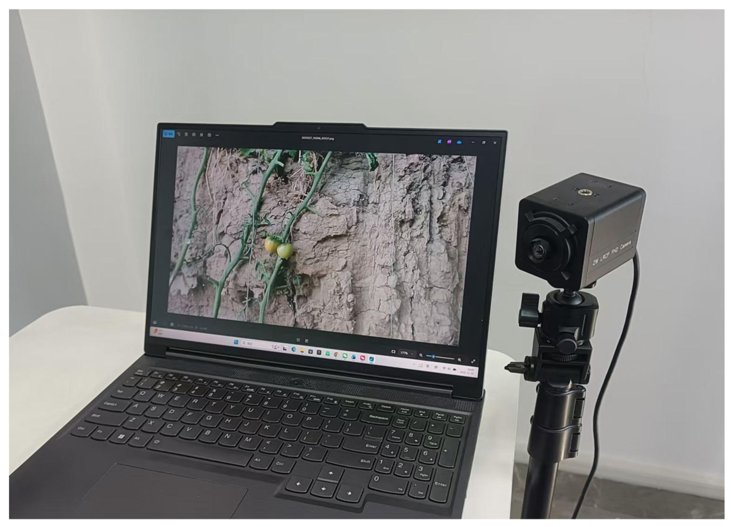
The data were collected from tomato greenhouses in Hohhot City, Inner Mongolia Autonomous Region, China (111°22′ E, 40°44′ N). An industrial camera (Shenzhen Zhongweiaoke Technology Co., Ltd., Shenzhen, China) was connected to a laptop Lenovo Y7000P (Lenovo Group, Beijing, China) for data acquisition, with the device parameters illustrated in Figure 1.

The equipment parameters are illustrated in

Table 1. Camera parameters.

Component	Specification
Model number	LRCP20680-PS1080P
Sensor	1/2.7 inch
Pixel size	3 µm × 3 µm
Focal length	3.6 mm
Fov	85
Resolution	1080 P
FPS	30
Interface	USB

.

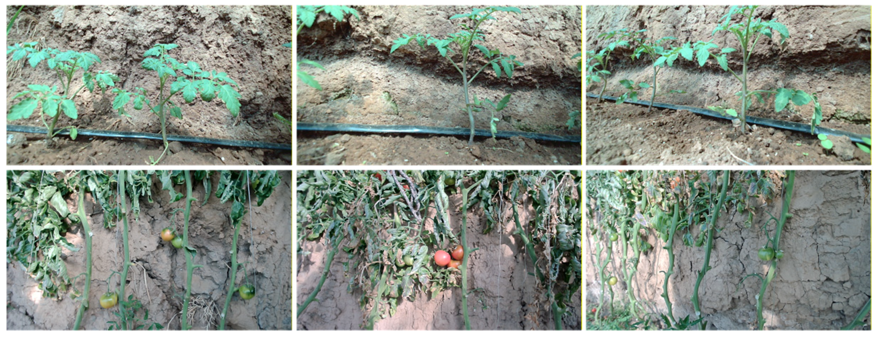
A total of 544 images were captured at a resolution of 1280 × 720 pixels. The dataset under consideration contains 247 images of tomato fruits during the fruiting stage. These images are used for fruit detection, ripeness recognition, and main stem and lateral branch segmentation. The dataset also includes 297 images of tomato stems and branches collected during the first two months of cultivation to augment the stem and branch data.

In order to ensure that the data collected on greenhouse-grown tomatoes reflected their natural growth state as closely as possible, the data collection process focused on two types of fruits: fully fruits and obscured fruits. Occluded fruits may be partially obscured by each other or by foliage. A subset of the captured fruits are partially within the camera’s field of view. The stem and branch images employed for segmentation encompass both complete and incomplete stems or branches. The image contains complete stems that extend from the top to the bottom, as well as incomplete stems and branches that may be partially obscured by foliage or intersect with other branches. The collated data are illustrated in Figure 2.

The initial row presents plant images during the seedling phase, while the subsequent row showcases tomatoes during the fruiting stage. The amalgamation of these 544 images constitutes a comprehensive tomato detection and segmentation dataset.

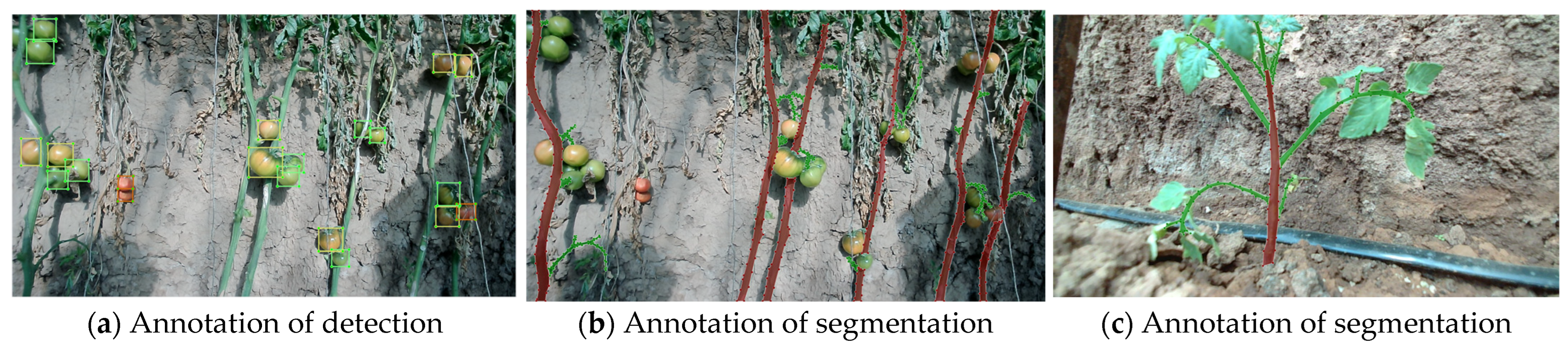
Two annotation methods were employed for the purpose of labeling the detection and segmentation tasks. To detect tomatoes, the LabelImg v1.8.6 program was employed to delineate bounding boxes, thereby categorizing tomatoes into three distinct ripeness stages: green stage (unripe tomatoes), turning stage (tomatoes beginning to ripe and turning to yellow), and ripe stage (fully red tomatoes). The segmentation of the main stem and lateral branches was achieved through the utilization of LabelMe v5.7.0, a software program designed for the segmentation task. The instances were divided into two distinct categories: main stem and lateral branch. The annotated data are illustrated in Figure 3.

A total of 544 image data points were annotated. The dataset was partitioned into training, validation, and test sets at a ratio of 7:1.5:1.5. Following the division of the original dataset, the training set comprised 384 images, the validation set contained 80 images, and the test set contained 80 images.

2.2. Data Augmentation

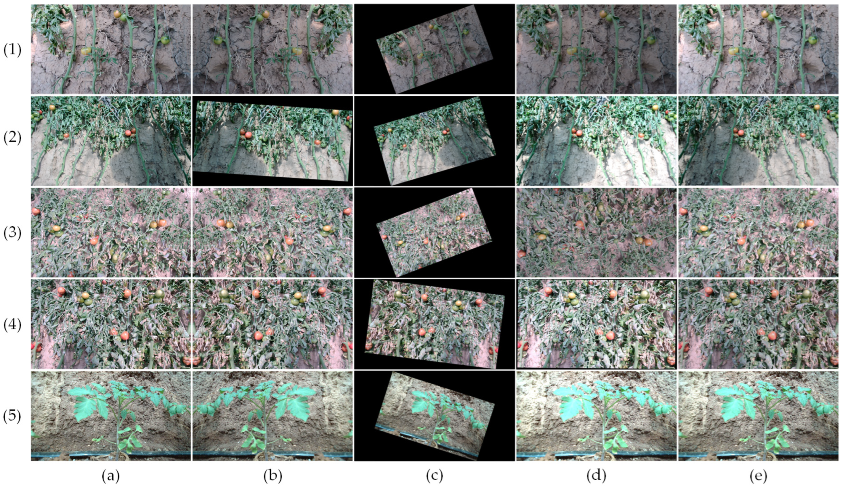
Following the partitioning of the dataset, the training set was expanded through the implementation of data augmentation techniques. The following methods were applied: horizontal flipping, vertical flipping, random rotation (from −30° to 30°), random scaling (from 0.8 to 1.2 scale), random cropping (from 0.7 to 1.0 scale), brightness adjustment (from 0.6 to 1.4 scale), Gaussian blur, and Gaussian noise. The detection and segmentation labels obtained were then subjected to identical transformations. The augmented training set comprised a total of 4224 images. The enhanced data are illustrated in Figure 4.

In real-world agricultural settings, the collection of tomato image data is susceptible to interference from factors such as varying angles, changing lighting conditions, and mutual occlusion among stems, branches, leaves, and fruits, leading to deviations in data representation. To address this challenge, targeted geometric and color transformations were applied through data augmentation techniques. This approach effectively expanded the dataset size while simulating the diverse conditions found in complex scenarios, significantly enhancing data diversity. This guided augmentation strategy enables models to learn more intrinsic, robust features that are unaffected by representational variations, thereby improving model generalization [20].

2.3. Data Dictionary

In accordance with the characteristics of multi-task learning, tomato detection labels and segmentation labels are concatenated to form new training data labels. The labels in this data dictionary are fully custom for the multi-task learning approach employed in this study. During the training phase, the newly generated labels are stored in a data dictionary format, as illustrated in

Table 2. Structure of the dataset dictionary.

Key	Value
{
im_file	Path of image file
shape	640 × 640
detect	Sub-dictionary for detection task
{
cls	Detect class labels
bboxes	Detect box labels
}
segment	Sub-dictionary for segmentation task
{
cls	Segmentation class labels
segments	Segmentation mask labels
}
}

.

The key “im_file” denotes the image storage path. The key “shape” denotes the training image resolution, which is set to 640 × 640.

The key “detect” is a sub-dictionary that contains detection labels. The key “cls” denotes the tomato ripeness labels, which use discrete numerical values: green stage is 0, turning stage is 1, and ripe stage is 2. The key “bboxes” denotes the tomato detection boxes and is stored in the (x, y, w, h) format. Here, (x, y) denotes the box’s position and (w, h) denotes its width and height.

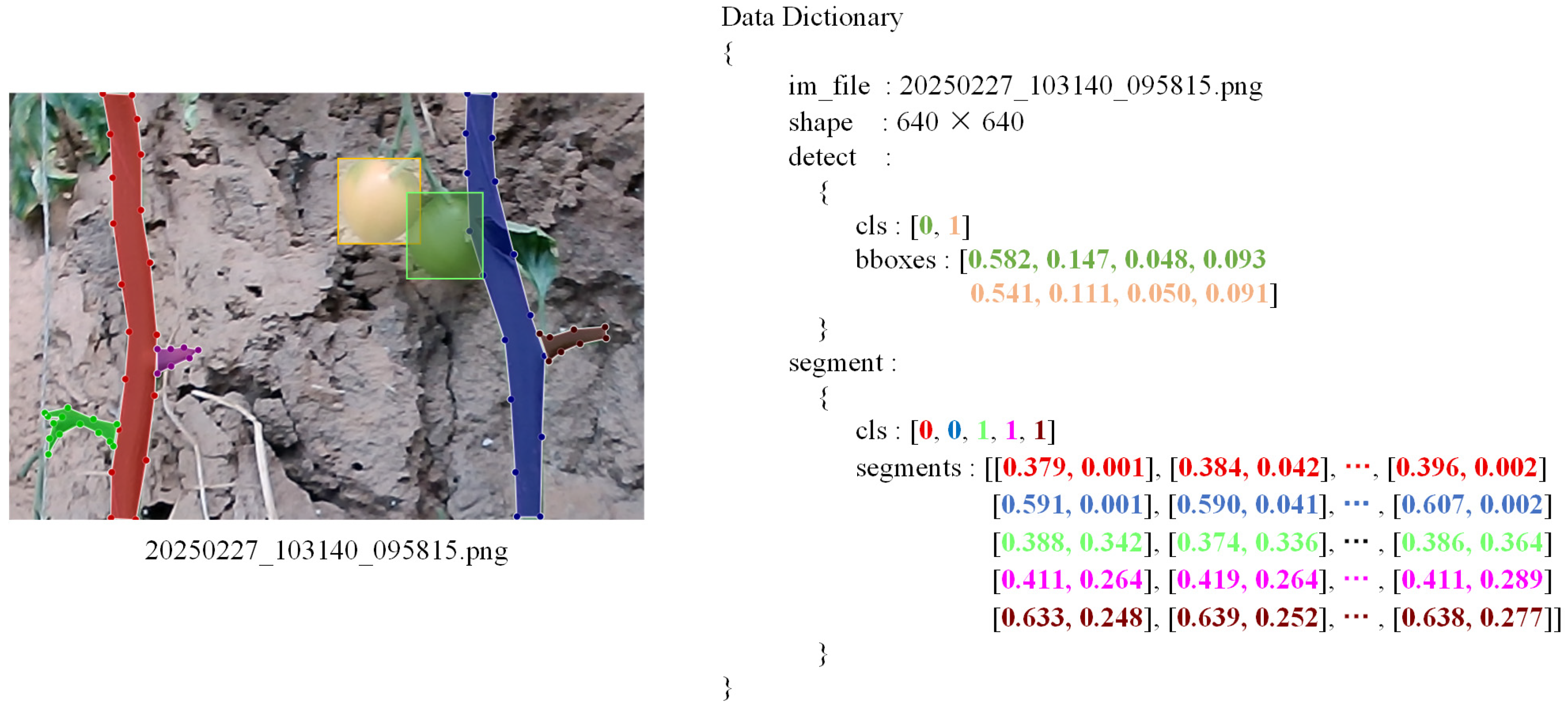
The key “segment” denotes sub-dictionary stores the segmentation labels. Here, key “cls” denotes the stem and branch categories: main stem is 0 and lateral branch is 1. The key “segments” denotes the segmentation masks. The data dictionary instance is illustrated in Figure 5.

The organization of tomato image annotation data is primarily divided into two sections: raw captured images are located on the left, and the data dictionary is located on the right. The utilization of a “color mark & structured label” approach facilitates the linkage of annotation data for detection and segmentation tasks. To facilitate differentiation, distinct color marks are applied to tomatoes, main stems, and lateral branches, with each object’s color mark corresponding to its label in the dictionary. Green tomatoes and turning tomatoes are annotated with green and yellow rectangles, respectively. The “detect” field in the data dictionary is used to store information regarding tomato category and location labels. The “cls” is employed for the storage of data pertaining to the tomato classes, and the integer 0 is assigned to indicate green tomatoes, while 1 is assigned to indicate tomatoes that are undergoing the process of color change. The “bboxes” are employed to store the tomato bounding boxes in a normalized (x, y, w, h) format. The image delineates two main stems, symbolized by red and dark blue polygons, respectively, and three lateral branches, represented by light green, pink, and brown polygons. The “segment” field in the data dictionary is used to store category and position labels. In this system, “cls” is employed to denote the classes, with 0 representing the main stem and 1 denoting the lateral branch. Segments are known to store masks as normalized (x, y) sequences. For instance, the red-labeled main stem corresponds to a polygon region bounded by vertices (0.379, 0.001), (0.384, 0.042), …, (0.396, 0.002), and so forth.

During the process of data augmentation, it is imperative to synchronously transform bounding boxes and masks. For instance, when applying rotation transformations, the bounding boxes of tomatoes should be synchronously rotated. In the process of computing masks, it is imperative to execute synchronous rotational transformations on the (x, y) sequences that are stored in segments. This will result in the generation of rotated polygons, thereby leading to the creation of synchronously augmented masks.

2.4. Improvements to the Model Based on the YOLOv8n

2.4.1. Model Structure of YOLOP-Tomato

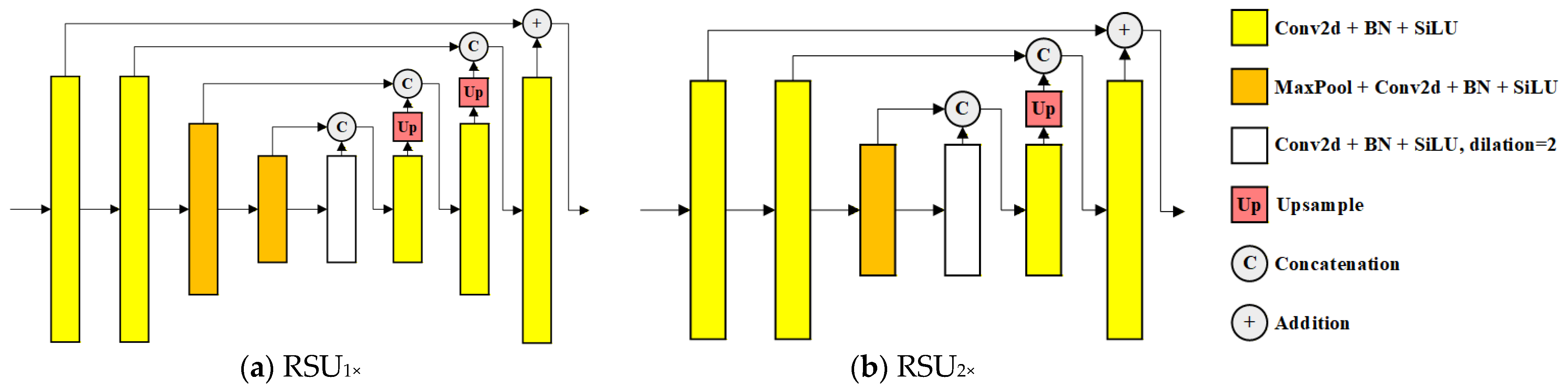
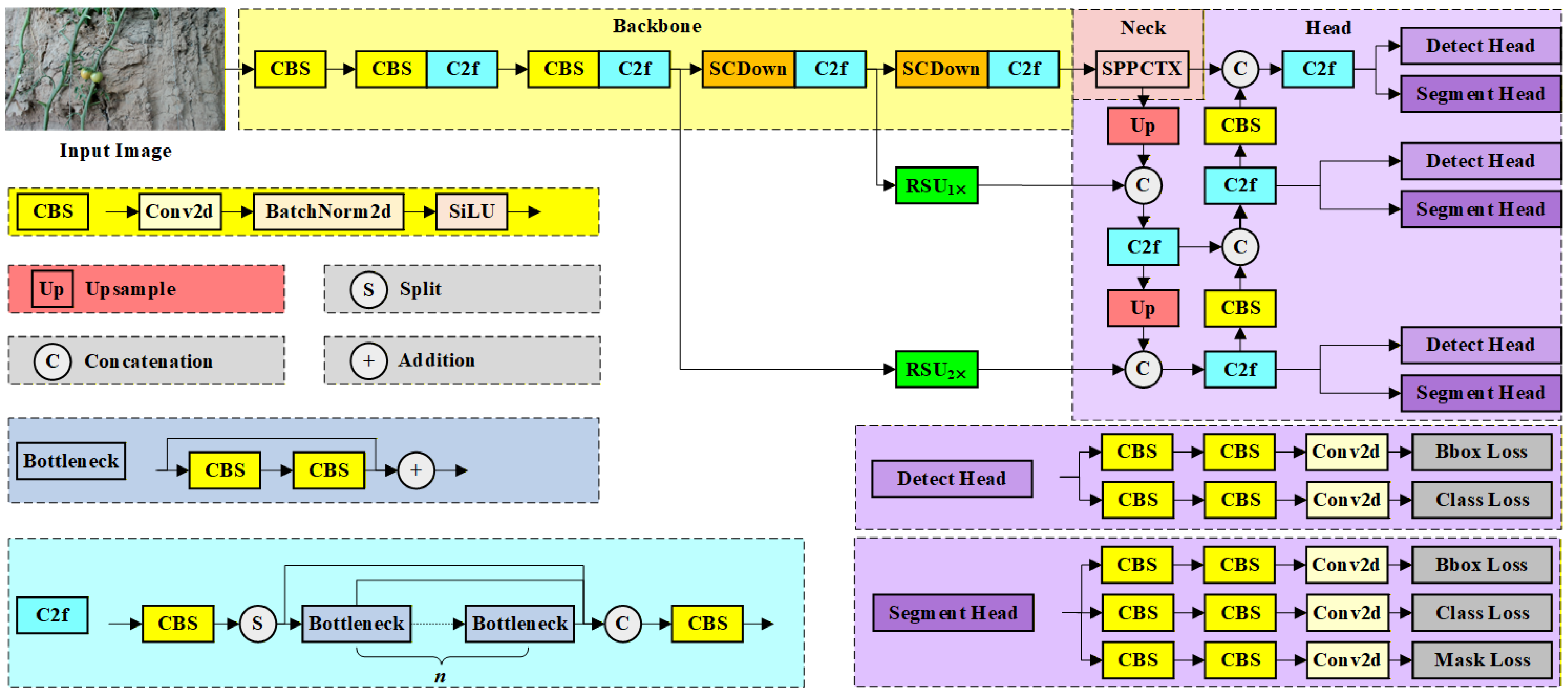
The improvements were derived from the YOLOv8n model, which was divided into three sections. Two RSU (residual U-blocks) modules were introduced between the backbone and head to construct a multi-scale feature enhancement path. The RSU module employs a U-Net-like encoder–decoder structure, integrating features across disparate levels through skip connections. In contrast to conventional single-stream convolutional U-Net architectures, the RSU modules offer enhanced gradient information and possess multi-scale receptive fields, thereby facilitating more effective extraction of detailed features from tomato fruits, stems, and branches. RSU1x and RSU2x represent 1x and 2x downsampling operations, respectively. In order to address the common challenges observed in tomato images, such as complex backgrounds and target misclassification, the SPPCTX module (SPP with context enhancement) has been developed as a replacement for the original SPPF structure in the neck. SPPCTX employs dilated convolutions to expand receptive fields, thereby effectively mitigating the feature weakening caused by overlapping or visually similar tomato fruits, stems, branches, or leaves. This enhancement of the model’s perception capabilities in complex scenes is a significant development. In the backbone, two SCDown (spatial-channel decoupled downsampling) modules replace the original CBS module. This results in network lightweighting while preserving feature extraction capability. The enhanced model is designated as YOLOP-Tomato (YOLO-Based Panoptic Perception for Tomato). The architectural design is illustrated in Figure 6.

2.4.2. ReSidual U-Blocks for Multi-Scale Feature Extraction

Tomatoes, stems, and branches exhibit distinct pixel-level characteristics. Due to the slender nature of stems and branches, instance segmentation poses greater challenges. To address this issue, the RSU module was incorporated into the model. The RSU module is designed as a U-Net-like structure comprising an encoder and a decoder. It employs skip connections to concatenate features from different levels of the encoder with corresponding features in the decoder, enabling multi-scale and deep feature extraction [21]. All convolutional kernels in the RSU module are 3 × 3 with a stride of 2. In the RSU_1× module, the encoder undergoes two convolutions, followed by a single max pooling operation. This results in the downsampling of the feature map to half resolution. Subsequent to this, a single convolution and a single dilated convolution are executed. The decoder first undergoes one convolution and one upsampling operation, concatenating the resulting feature map with the corresponding layer from the encoder. Subsequent to a final convolution, the output is integrated with the initial layer’s convolution output from the encoder, thereby yielding the final output. The overall structure of RSU_2× is analogous to that of RSU_1×, with the exception of the encoder, which utilizes double downsampling by repeating the max-pooling and convolution operations twice. The decoder employs two consecutive convolutions followed by upsampling. The RSU module is illustrated in Figure 7.

2.4.3. SPP with Context Enhancement Module

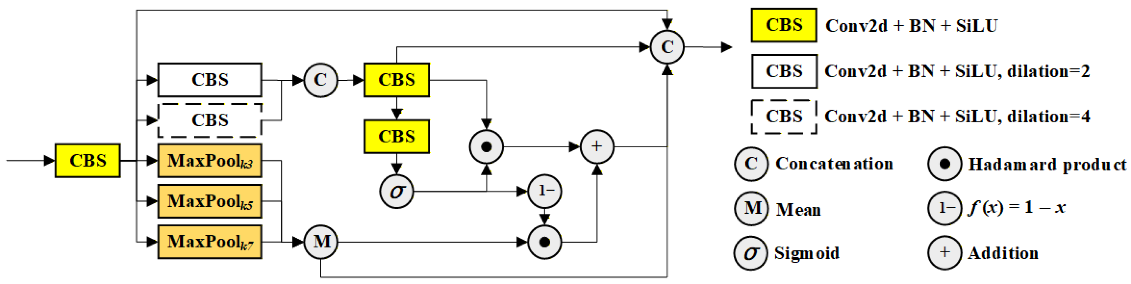
Multi-scale contextual features have been identified as a critical method for enhancing the accuracy of computer vision models. Conventional SPP modules attain multi-scale feature fusion through the implementation of stacked max-pooling layers, thereby establishing the basis for subsequent multi-scale feature extraction modules [22]. Attention mechanisms have emerged as a prevalent approach for enhancing contextual feature extraction in visual models. These mechanisms facilitate feature weighting, guiding models to prioritize more significant features [23]. In natural environments, tomato fruits and foliage exhibit irregular growth patterns, with fruits often obscured by leaves or branches, leading to feature weakening. Occlusion disperses effective tomato features across different regions, causing discontinuity and fragmentation. This increases the difficulty of feature extraction, causing models to learn more irrelevant features while neglecting the fruit. To address this issue, a context-feature-enhancing neck module is proposed. This module employs max-pooling layers to generate a feature pyramid, leveraging dilated convolutions to extract multi-scale contextual features [24]. Subsequently, weights are derived based on contextual information, and an adaptive fusion with pooled features is performed. This process enhances the associative fusion capability of multi-scale features. The specific computational process is presented in Equations (1)–(6),

$$x=\mathrm{C}\mathrm{B}\mathrm{S}\left(x_{in}\right)$$

(1)

$$x_c=\mathrm{C}\mathrm{B}\mathrm{S}\left(\mathrm{C}\mathrm{o}\mathrm{n}\mathrm{c}\mathrm{a}\mathrm{t}\right({\mathrm{C}\mathrm{B}\mathrm{S}}_{d2}\left(x\right),{\mathrm{C}\mathrm{B}\mathrm{S}}_{d4}\left(x\right)\left)\right)$$

(2)

$$x_p=\mathrm{M}\mathrm{e}\mathrm{a}\mathrm{n}\left({\mathrm{M}\mathrm{a}\mathrm{x}\mathrm{P}\mathrm{o}\mathrm{o}\mathrm{l}}_{k3}\left(x\right),{\mathrm{M}\mathrm{a}\mathrm{x}\mathrm{P}\mathrm{o}\mathrm{o}\mathrm{l}}_{k5}\left(x\right),{\mathrm{M}\mathrm{a}\mathrm{x}\mathrm{P}\mathrm{o}\mathrm{o}\mathrm{l}}_{k7}\left(x\right)\right)$$

(3)

$$w=\sigma \left(\mathrm{C}\mathrm{B}\mathrm{S}\left(x_c\right)\right)$$

(4)

$$x_w=w⨀x_c+\left(1-w\right)⨀x_p$$

(5)

$$x_{out}=\mathrm{C}\mathrm{o}\mathrm{n}\mathrm{c}\mathrm{a}\mathrm{t}\left(x,x_c,x_p,x_w\right)$$

(6)

where the $x_{in}$ denotes the input feature, and CBS is employed to represent a standard convolutional block comprising a convolutional layer, a batch normalization layer, and a SiLU activation layer. The ${\mathrm{C}\mathrm{B}\mathrm{S}}_{d2}$ and ${\mathrm{C}\mathrm{B}\mathrm{S}}_{d4}$ represent dilated convolutional blocks with dilation factors of 2 and 4, respectively. Concat represents feature concatenation along the channel dimension. The extraction of contextual features, denoted by $x_c$, is achieved through the implementation of dilated convolution. The ${\mathrm{M}\mathrm{a}\mathrm{x}\mathrm{P}\mathrm{o}\mathrm{o}\mathrm{l}}_{kn}$ refers to a max-pooling layer with a kernel size of n, while Mean represents the mean function. Subsequent to element-wise averaging of the multi-scale pooling outputs, the pooled features, denoted by $x_p$, are obtained. The symbol $\sigma$ is used to denote the Sigmoid function. The feature weights are obtained via Equation (4), and Equation (5) performs linear weighting of the contextual and pooled features to yield $x_w$. The symbol $⨀$ denotes the Hadamard product. In conclusion, the enhanced multi-scale fused contextual feature $x_{out}$ is obtained by concatenating $x$, $x_c$, $x_p$, and $x_w$. The module structure of SPPCTX is illustrated in Figure 8.

2.4.4. Spatial-Channel Decoupled Downsampling Module

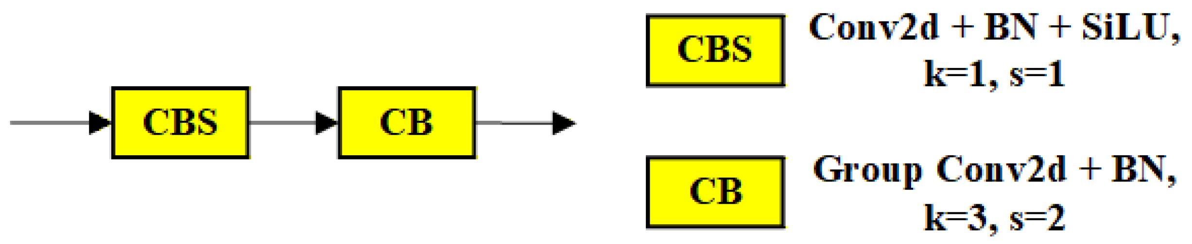
In the YOLOv8 model, downsampling and channel reduction are typically implemented using standard convolutions. In order to fully extract features, it is often necessary to increase the number of channels in feature maps. However, this results in a significant increase in the computational overhead of convolutions. The SCDown module has been demonstrated to decouple spatial sampling operations from channel variation operations, thereby effectively reducing the number of parameters while preserving the module’s feature extraction capability [25]. This work implements the SCDown module in the deeper layers of the YOLOP-Tomato backbone, replacing the original CBS module to reduce overall computational complexity. The module structure of SCDown is illustrated in Figure 9.

The first CBS layer consists of a standard convolution with a kernel size of 1 and a stride of 1, a batch normalization layer, and a SiLU activation layer. This process results in an augmentation of the number of channels from c to 2c. The second convolutional layer, designated as CB, comprises group convolutions with a kernel of 3 and a stride of 2, and a batch normalization layer. Grouping is configured to 2c, thereby facilitating feature extraction and downsampling.

2.5. Loss Function

The loss function of the YOLOP-Tomato model comprises classification, regression, and segmentation losses to optimize multi-task detection and segmentation. The classification loss uses the BCE (binary cross entropy) loss function, as presented in Equation (7),

$${Loss}_{cls}=-{\displaystyle \frac{1}{N}}\sum _{i=1}^N\left({y_i}^{\mathrm{g}\mathrm{t}}·\mathrm{l}\mathrm{o}\mathrm{g}\left({y_i}^{\mathrm{p}\mathrm{r}\mathrm{e}\mathrm{d}}\right)+\left(1-{y_i}^{\mathrm{g}\mathrm{t}}\right)·\mathrm{l}\mathrm{o}\mathrm{g}\left(1-{y_i}^{\mathrm{p}\mathrm{r}\mathrm{e}\mathrm{d}}\right)\right)$$

(7)

where N denotes the number of samples, ${y_i}^{\mathrm{g}\mathrm{t}}$ denotes the ground truth of the samples, and ${y_i}^{\mathrm{p}\mathrm{r}\mathrm{e}\mathrm{d}}$ denotes the model’s predicted output.

The regression loss is computed using a combination of DFL (Distribution Focal Loss) and CIoU (Complete Intersection over Union). In the context of bounding box prediction, the model initially generates a probability distribution over discrete intervals. The predicted bounding box coordinates are subsequently obtained by applying a weighted probability distribution, as presented in Equation (8),

$$y_{box}=\sum _{i=0}^{15}\mathrm{S}\mathrm{o}\mathrm{f}\mathrm{t}\mathrm{m}\mathrm{a}\mathrm{x}\left({p_i}^{\mathrm{p}\mathrm{r}\mathrm{e}\mathrm{d}}\right)·i$$

(8)

where i = 0, 1, 2, …, 15, the probability interval points are represented, and ${p_i}^{\mathrm{p}\mathrm{r}\mathrm{e}\mathrm{d}}$ denotes the predicted discrete coordinate values for the $ith$ interval. The coordinate probability distribution is obtained using the Softmax function, and the bounding box coordinates are derived through linear weighting.

The boundary loss is computed using the DFL, as presented in Equation (9),

$${Loss}_{dfl}=-\left((y_{i+1}-y^{\mathrm{g}\mathrm{t}})·\mathrm{l}\mathrm{o}\mathrm{g}(\mathrm{S}\mathrm{o}\mathrm{f}\mathrm{t}\mathrm{m}\mathrm{a}\mathrm{x}({p_i}^{\mathrm{p}\mathrm{r}\mathrm{e}\mathrm{d}}))+(y^{\mathrm{g}\mathrm{t}}-y_i)·\mathrm{l}\mathrm{o}\mathrm{g}(\mathrm{S}\mathrm{o}\mathrm{f}\mathrm{t}\mathrm{m}\mathrm{a}\mathrm{x}({p_{i+1}}^{\mathrm{p}\mathrm{r}\mathrm{e}\mathrm{d}}))\right)$$

(9)

where i denotes a point within the probability interval and $y^{\mathrm{g}\mathrm{t}}$ denotes the true coordinate, $y_i$ denotes the left endpoint of $y^{\mathrm{g}\mathrm{t}}$, obtained by rounding y^gt down, and $y_{i+1}$ denotes the right endpoint of $y^{\mathrm{g}\mathrm{t}}$, obtained by rounding $y^{\mathrm{g}\mathrm{t}}$ up. ${p_i}^{\mathrm{p}\mathrm{r}\mathrm{e}\mathrm{d}}$ and ${p_{i+1}}^{\mathrm{p}\mathrm{r}\mathrm{e}\mathrm{d}}$ denotes the model’s predicted values at the $ith$ and $i+1th$ interval points, respectively.

The intersection-over-union loss for bounding boxes is computed by a CIoU metric, as presented in Equation (10),

$${Loss}_{box}=1-IoU+{\displaystyle \frac{{\rho }^2\left(b,b^{gt}\right)}{c^2}}+\alpha v$$

(10)

where $IoU$ denotes the intersection-over-union ratio between the predicted and ground truth bounding boxes, $b$ denotes the center coordinates of the predicted bounding box, $b^{gt}$ denotes the center coordinates of the ground truth bounding box, ${\rho }^2\left(b,b^{gt}\right)$ denotes the Euclidean distance from $b$ to $b^{gt}$, and $c^2$ denotes the diagonal distance between the minimum bounding rectangles of the predicted and ground truth bounding boxes. The values of $v$ and $\alpha$ are defined as presented in Equations (11) and (12),

$$v={\displaystyle \frac{4}{{\pi }^2}}\left({\tan }^{-1}{\displaystyle \frac{w^{gt}}{h^{gt}}}-{\tan }^{-1}{\displaystyle \frac{w^{pred}}{h^{pred}}}\right)$$

(11)

$$\alpha ={\displaystyle \frac{v}{\left(1-IoU\right)+v}}$$

(12)

where $w^{gt}$ and $h^{gt}$ denote the width and height of the ground truth bounding box, respectively. Similarly, $w^{pred}$ and $h^{pred}$ denote the width and height of the predicted bounding box. The weighting coefficient, denoted by $\alpha$, is determined based on the $IoU$ metric and the value of $v$.

During the segmentation process, the segment head generates a set of prototype masks with a resolution of 160 × 160 × 32. Linear weighting of these prototype masks results in the prediction of a mask for the target instance, with a resolution of 160 × 160 × 1. The segmentation head also includes a branch for computing the bounding box of the segmented instance. Subsequent to determining the instance size via Equation (8), bilinear interpolation is employed to resample the predicted mask to the same dimensions as the bounding box. The mask loss is computed using the BCE function, as presented in Equation (13),

$${Loss}_{mask}=-{\displaystyle \frac{1}{N}}\sum _{i=1}^N\left({y_i}^{\mathrm{g}\mathrm{t}}·\mathrm{l}\mathrm{o}\mathrm{g}\left({y_i}^{\mathrm{p}\mathrm{r}\mathrm{e}\mathrm{d}}\right)+\left(1-{y_i}^{\mathrm{g}\mathrm{t}}\right)·\mathrm{l}\mathrm{o}\mathrm{g}\left(1-{y_i}^{\mathrm{p}\mathrm{r}\mathrm{e}\mathrm{d}}\right)\right)$$

(13)

where N denotes the number of samples, ${y_i}^{\mathrm{g}\mathrm{t}}$ denotes the ground truth of the mask, and ${y_i}^{\mathrm{p}\mathrm{r}\mathrm{e}\mathrm{d}}$ denotes the model’s predicted mask.

2.6. Evaluation Indicators

The model’s performance for the tomato detection task is validated using precision (P), recall (R), and average precision (AP) metrics, while the model’s performance for the segmentation task is validated using the intersection over union (IoU) metric. The relevant evaluation metrics are presented in Equations (14)–(17),

$$Precision={\displaystyle \frac{TP}{TP+FP}}\times 100\%$$

(14)

$$Recall={\displaystyle \frac{TP}{TP+FN}}\times 100\%$$

(15)

$$AP={\mathsf{\int }}_0^{1}PRdR$$

(16)

$$IoU={\displaystyle \frac{TP}{TP+FP+FN}}\times 100\%$$

(17)

where $TP$ denotes true positives, $FP$ denotes false positives, and $FN$ denotes false negatives. In Equation (17), $TP$, $FP$, and $FN$ are calculated at the pixel level to compute segmentation $IoU$.

3. Results

3.1. Training Parameters Setting

All experiments were executed on an NVIDIA RTX 2080 Ti, equipped with 8GB of VRAM. The system component is illustrated in

Table 3. System component and specification.

Component	Specification
CPU	Intel(R) Core(TM) i7-8700k CPU @ 3.70 GHz
GPU	NVIDIA RTX 2080 Ti
GPU Memory	8 GB
Cuda	12.6

.

The training epoch is set to 200 rounds, with a batch size of 16, determined by the available GPU memory. During each training iteration, a set of techniques, including translation, scaling, horizontal flipping, copy–paste, HSV, and mosaic enhancement are applied to enhance the model’s robustness. The model training hyperparameters are illustrated in

Table 4. Setting of training hyperparameters and value.

Hyperparameter	Value
Image size	640 × 640
Epochs	200
Batch size	16
Optimizer	AdamW
Momentum	0.937
Weight decay	0.0005
Learning rate	0.01
Seed	0

.

In order to circumvent the potential interference from random factors such as data processing and parameter initialization during the training process and final performance evaluation, this study fixed the random seed to 0 during the model training phase.

3.2. Data Imbalance and Mitigation Techniques

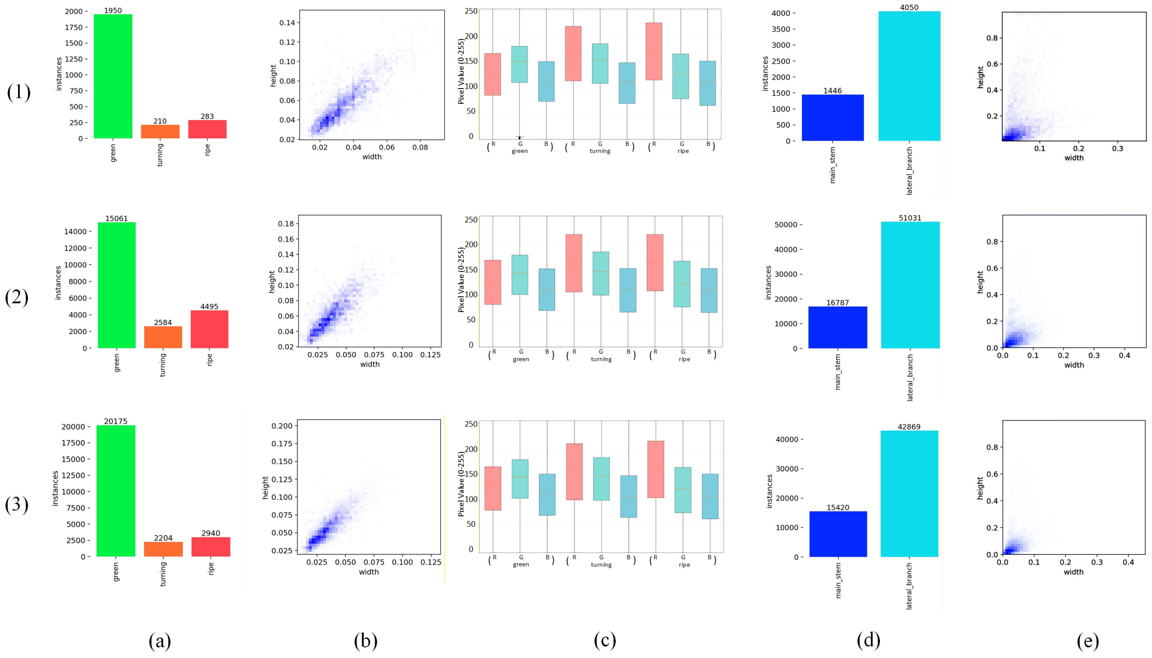
The original dataset contains 1950 instances of green tomatoes, 210 instances of turning tomatoes, and 283 instances of ripe tomatoes. The presence of unripe fruits is more pronounced. In general, the occurrence of tomato instances is limited, and compared to green tomatoes, the number of ripe and turning tomato instances is smaller. This necessitates dataset augmentation to expand the data. Two data augmentation strategies were employed. The first utilized oversampling, selecting images of turning and ripe tomatoes for augmentation. This expanded the number of images primarily containing turning and ripe tomatoes by 20 times, while increasing the number of images primarily containing green tomatoes by 5. The second augmented the entire dataset by a factor of 10.

During the process of dataset augmentation, the enhancement methods employed, as delineated in Section 2.2, encompassed horizontal flipping, vertical flipping, rotation, scaling, cropping, brightness adjustment, Gaussian blur, and Gaussian noise. The specific enhancement methods and their corresponding parameters are illustrated in

Table 5. Parameters used during data augmentation.

Method	Parameter	Value 1
Rotation	Degree range	±30°
Scale	Scale range	0.8–1.2
Crop	Crop range	0.7–1.0
Brightness	Brightness range	0.6–1.4
Gaussian blur	Kernel size range	3–5
Gaussian noise	Variance range	5–30

.

The fruit of the tomato plant is typically spherical or elliptical in shape. An expanded range of rotation angles could enhance data diversity; however, it is imperative to exercise caution and avoid excessive rotation, as this may result in the alteration of the orientation of the main stem and lateral branches. Consequently, the rotation angle is set to ±30°. The scale range has been set to 0.8–1.2, ensuring that the pixel proportion of instances aligns with the original dataset distribution. Given the relatively diminutive mask pixel proportions and slender shapes exhibited by certain lateral branches, an excessively broad crop range would result in the discarding of a substantial number of valid pixels. The crop range is set to 0.7–1.0 to prevent damaging segmentation instances and masks. The brightness setting is adjusted to a range of 0.6–1.4. Given that the width-to-height ratio of tomatoes and some lateral branches ranges from 0.02 × 0.02 to 0.08 × 0.06, the Gaussian blur kernel size range is set to 3–5. The range of the Gaussian noise variance is set to 5–30, thereby facilitating the application of localized blurring and noise. During the data augmentation process, two–three methods are randomly selected to transform the same image.

A comparison of the distributions of classes, bounding boxes, and masks between the original training set and the augmented training set was conducted to assess the similarity between the augmented data and the original data distributions. The results of this study are presented in Figure 10.

As demonstrated in Figure 10, the ratios of green, turning, and ripe after expansion using Strategy 1 are 15,061:2584:4495. The ratios subsequent to expansion employing Strategy 2 are 20,175:2204:2940. Observation (b) indicates that the overall height and width distributions of bounding boxes subsequent to expansion by both strategies demonstrate a resemblance to those of the original training set, with heights ranging from [0.02, 0.08] and widths from [0.02, 0.06], exhibiting a positive correlation overall. Given the high degree of similarity in the overall appearance and texture of tomatoes, color information becomes a pivotal factor in their classification. Observation (c) demonstrates that following the utilization of the brightness-enhanced dataset, the aggregate RGB channel distributions for green, turning, and ripe tomato targets exhibit a high degree of similarity, thereby ensuring consistency in color distribution across the augmented dataset. A quantitative analysis of the mask distribution of segmented instances in (d) reveals that the ratio of main stem to lateral branches remains approximately 2.5:7.5, indicating a relatively stable proportion between these two components. Following the implementation of ±30° rotation, observing (e) shows that the width and height distribution of the augmented masks generally aligns with the original training set.

The baseline model YOLOv8n was trained to compare the impact of different strategies on various metrics. Despite the augmentation of the dataset, which led to an increase in both the number and diversity of instances, the overall sample distribution remained imbalanced. For instance, green tomatoes continued to outnumber both turning and ripe tomatoes. Consequently, the implementation of dynamic data augmentation techniques during the training process led to a notable enhancement in the model’s generalization capability and a substantial reduction in category imbalance. The analysis was conducted across multiple dimensions, including precision (P), recall (R), mAP₅₀, mAP_50–95 for tomato detection, and mIoU for instance segmentation, and the results are illustrated in

Table 6. Data augmentation parameters used during training.

Method	Parameters	Probability
Mosaic	4	100%
Copy paste	-	50%
Translate	0.1	100%
Scale	0.5	100%
Horizontal flip	-	50%

.

After expanding the dataset, YOLOv8n was employed as the baseline model for testing to evaluate the performance of the expanded datasets under different strategies. The analysis was conducted across multiple dimensions, including precision (P), recall (R), mAP₅₀, mAP_50–95 for tomato detection, and mIoU for instance segmentation, and the results are illustrated in

Table 7. Comparison of different data augmentation strategies.

Strategy	Detection	P	R	mAP50	mAP50–95	Segmentation	mIoU
	Class	(%)	(%)	(%)	(%)	Class	(%)
1	All	91.5	86.4	92.4	60.5	All	72.9
	Green	90.2	79.8	90.2	52.7	Main stem	78.8
	Turning	89.8	88.2	91.6	62.4	Lateral branch	67.1
	Ripe	94.5	91.2	95.5	66.4
2	All	92.4	84.9	93.1	59.8	All	76.2
	Green	90.6	80.5	91.7	53.0	Main stem	85.0
	Turning	91.0	86.0	93.1	63.3	Lateral branch	67.4
	Ripe	95.5	88.2	94.6	63.2

.

Training data enhanced using Strategy 1 are highly recall-friendly, achieving an overall recall rate of 86.4%, with recall rates of 88.2% and 91.2% for turning and ripe tomatoes, respectively. The efficacy of Strategy 1, which involves the oversampling of mature tomatoes, was demonstrated by the mAP₅₀ and mAP_50–95, which reached 95.5% and 66.4%, respectively. The application of Strategy 2 generally yields superior outcomes in precision metrics when compared with Strategy 1. For mAP₅₀, Strategy 2 attains 91.7% for green tomatoes and 93.1% for turning tomatoes. In mAP_50–95, it achieves 53.0% for green tomatoes and 63.3% for turning tomatoes, surpassing Strategy 1. In the concurrent segmentation task, Strategy 2 achieved mIoU scores of 85.0% for main stems and 67.4% for lateral branches, thereby demonstrating superior performance in both categories when compared to Strategy 1. In summary, Strategy 1 prioritizes the recall, mAP₅₀, and mAP_50–95 metrics for accurately predicting the ripeness of tomatoes by increasing their representation in the dataset. Conversely, Strategy 2 exhibited a marked predilection for predicting precision, mAP₅₀, and mAP_50–95 for green and turning tomatoes. When taking into account the mIoU metric for segmentation tasks, Strategy 2 emerges as a more balanced choice overall. Consequently, the dataset that was trained using Strategy 2 is selected for further analysis.

3.3. Ablation Experiments

To investigate the impact of RSU, SPPCTX, and SCDown on model performance, eight comparative experiments were designed with YOLOv8n as the baseline. The evaluation indicators included precision (P), recall (R), mAP₅₀, mAP_50–95 for tomato detection, mIoU for instance segmentation, and inference speed. In order to mitigate hardware load fluctuations, the inference speed is reported as the average of ten repeated experiments, rounded to two decimal places. The results of this study are illustrated in

Table 8. Training results for different modules.

Id	RSU	SPPCTX	SCDown	P	R	mAP50	mAP50–95	mIoU	Speed
				(%)	(%)	(%)	(%)	(%)	(ms)
1 (baseline)				92.4	84.9	93.1	59.8	76.2	8.01
2	√			94.8	83.9	92.7	60.3	77.6	8.13
3		√		93.0	82.8	93.0	61.8	77.2	7.54
4			√	88.3	88.7	93.3	61.7	78.0	7.91
5	√	√		90.3	84.6	92.9	60.8	74.7	7.62
6	√		√	91.2	83.6	93.1	62.0	76.5	7.92
7		√	√	90.6	86.9	92.6	60.7	77.9	8.03
8	√	√	√	94.9	85.0	93.6	60.9	77.6	8.14

.

Among single-module performances, to integrate multi-scale instance features and enhance the representational power of tomatoes, stems and branches, the RSU module (Id = 2) was employed, achieving a precision of 94.8% and an mIoU of 77.6%, the precision, mAP_50–95, and mIoU value increased by 2.4%, 0.5%, 0.1%, and 1.4%, though recall and mAP₅₀ experienced slight reductions. The SPPCTX module (Id = 3) enhanced mAP_50–95 to 61.8% and optimized inference speed to 7.54 ms, thereby attaining the optimal performance across all experiments. On the one hand, the SPPCTX enhances the system’s robustness toward tomato targets, elevating the mAP_50–95 and mIoU. On the other hand, the substitution of traditional convolutions with dilated convolutions has been demonstrated to reduce computational complexity. The SCDown module (Id = 4) demonstrated a significant enhancement in recall, achieving 88.7%, and in mIoU, reaching 78.0%. These outcomes were the most optimal across all experimental iterations. However, the accuracy of tomato detection did not reach 90%, suggesting the potential for enhancement. With respect to the configuration of modules, the combination of RSU and SCDown (Id = 6) yielded the maximum mAP_50–95 of 62.0%. The combination of SPPCTX and SCDown (Id = 7) exhibited high recall (86.9%) and mIoU (77.9%), the recall, mAP_50–95, and mIoU value increased by 2.0%, 0.9%, and 1.7%, The integration of SCDown and SPPCTX produces a more comprehensive array of features, facilitating the aggregation of context information to facilitate a more focused examination of the tomato target region. This reduction in background interference enhances target localization, thereby optimizing segmentation accuracy while maintaining high recall rates.

When all three were used in conjunction (Id = 8), precision (94.9%), and mAP₅₀ (93.6%) achieved optimal values, while recall (85.0%) and mIoU (77.6%) ranked among the top three. Although mAP_50–95 (60.9%) ranked fourth, 1.1% lower than the optimal value (Id = 6, 62.0%), it demonstrated a 1.1% improvement over the baseline model (59.8%). Compared to the baseline, the precision, recall, mAP_50, mAP_50–95, and mIoU value increased by 2.5%, 0.1%, 1.5%, 1.1%, and 1.4%. Furthermore, the inference speed of the three-module combination was 8.14 ms, which is comparable to the baseline model. This demonstrates that the three proposed improvement modules form an efficient synergistic complementary effect. Specifically, the structural optimization of the original model not only captures multidimensional feature flow information more accurately, significantly enhancing the model’s multi-scale feature extraction capability and feature fusion efficiency, but also effectively controls model complexity while improving core metrics such as tomato detection accuracy and stem–branch segmentation precision. The synergistic interaction among these three components collectively drives a comprehensive performance enhancement in tomato detection and stem–branch segmentation tasks.

In summary, the combination of three modules (Id = 8) achieves the optimal balance between accuracy and performance, demonstrating a clear advantage in detection accuracy and providing an effective reference for model structure optimization.

3.4. Performance Comparison and Analysis

3.4.1. Comparison with Foundational Models

To further evaluate the performance of YOLOP-Tomato, this study selected main-stream models for comparison, including Faster R-CNN, SSD, RT-DETR-l, YOLOv5n, YOLOv8n, YOLOv10n, and YO-LO11n. These models were trained under identical experimental environments and parameter conditions, and their performance was assessed using the test set. The results are illustrated in

Table 9. Training results for different models.

Model	P	R	mAP50	mAP50–95	mIoU	FLOPs	Size	Speed
	(%)	(%)	(%)	(%)	(%)	(G)	(MB)	(ms)
Faster R-CNN [26]	58.1	85.9	80.4	39.1	-	474.1	110.9	103.51
SSD [27]	92.8	71.1	86.2	43.7	-	29.62	47.4	100.62
RT-DETR-l [28]	91.6	84.3	91.1	60.1	-	103.4	64.6	18.65
YOLOv5n [29]	91.0	83.5	92.6	61.1	75.7	13.3	7.2	8.16
YOLOv8n [30]	92.4	84.9	93.1	59.8	76.2	14.3	8.2	8.01
YOLOv10n [25]	87.9	85.9	91.7	60.7	76.5	11.5	6.2	7.97
YOLO11n [30]	88.7	85.6	92.0	61.4	76.6	11.3	6.8	8.01
YOLOP-Tomato	94.9	85.0	93.6	60.9	77.6	16.9	9.6	8.14

.

As illustrated in Table 9, Faster R-CNN, SSD, and RT-DETR-l represent classic object detection models. These models were utilized to execute the tomato detection task and were subsequently compared against the object detection metrics within the YOLOP-Tomato multi-task framework.

YOLOP-Tomato attained an optimal precision of 94.9%, signifying more precise classification decisions for tomatoes and a substantial reduction in false detection rates. The YOLOv10n model demonstrated the highest recall rate of 85.9%, while the YO-LO-Tomato model exhibited a recall of 85.0%, indicating a marginal difference of 0.9% between the two models. This observation underscores the efficacy of the YOLOv10n model in capturing features of tomatoes with notable precision. The two models demonstrate a high level of proficiency in reducing false negatives in the classification of tomatoes. This suggests that they are capable of comprehensive feature capture for tomatoes. YOLOP-Tomato attains an optimal mAP₅₀ of 93.6%, signifying its superior performance. At mAP_50–95, YOLOP-Tomato achieves a 60.9% success rate, placing it among the top three models. With regard to mIoU, YOLOP-Tomato achieves a leading score of 77.6%, signifying its proficiency in differentiating stem semantic information. This attribute renders it particularly well-suited for scenarios that demand precise segmentation, such as in agricultural contexts. In terms of FLOPs, YOLOP-Tomato consumes 16.9 G, reflecting increased computational overhead due to its three optimization modules. The model size is 9.6 MB, indicating that multi-task optimization introduces storage overhead but remains within the lightweight model category. YOLOP-Tomato demonstrates an inference speed of 8.14 ms, which generally meets real-time detection requirements.

In summary, YOLOP-Tomato offers a valuable trade-off between accuracy and efficiency.

3.4.2. Performance Evaluation on Tomato Ripeness Detection

To assess the efficacy of various models in the tomato detection task, a comparative analysis was conducted on the detection results for three distinct tomato ripeness stages: green, turning, and ripe. The evaluation metrics employed included precision (P), recall (R), and AP₅₀. The results are illustrated in

Table 10. Training results for detection task of different models.

Model	P			R			AP50
	(%)			(%)			(%)
	Green	Turning	Ripe	Green	Turning	Ripe	Green	Turning	Ripe
Faster R-CNN	48.9	63.8	61.5	83.0	88.0	86.8	73.3	82.3	85.4
SSD	90.9	91.1	96.5	50.5	82.0	80.9	75.2	92.4	91.1
RT-DETR-l	88.4	90.8	95.6	77.1	86.0	89.7	89.7	87.6	96.1
YOLOv5n	94.5	89.2	89.4	81.2	84.0	85.3	93.2	92.7	92.0
YOLOv8n	90.6	91.0	95.5	80.5	86.0	88.2	91.7	93.1	94.6
YOLOv10n	88.5	88.0	87.2	80.9	90.0	86.8	90.0	92.0	93.1
YOLO11n	90.0	86.7	89.5	81.4	90.0	85.3	91.7	93.8	90.7
YOLOP-Tomato	95.5	93.5	95.7	75.8	88.0	91.2	91.9	93.6	95.3

.

Among these, YOLOP-Tomato demonstrated exceptional precision, ranking first in the green (95.5%) and turning (93.5%) categories. Its ripe (95.7%) accuracy was second only to SSD (96.5%). This finding suggests that the model exhibits exceptional accuracy in tomato classification, effectively distinguishing between tomato and background. Concurrently, the capacity of model to accurately detect the onset of tomato turning is indicative of its aptitude for effectively mitigating the misclassification of turning fruit as green or ripe. YOLOP-Tomato demonstrated a recall rate of 91.2% for ripe tomatoes, the highest among all models, indicating the lowest false negative rate for ripe tomatoes. For turning tomatoes, the recall reached 88.0%, placing it in third position overall. However, it is important to note that the recall for green tomatoes was 75.8%, indicating a substantial opportunity for enhancement in this particular category. YOLOP-Tomato attained an AP₅₀ of 91.9% for green stage tomatoes, placing second behind YOLOv5n with an AP₅₀ of 93.2%. For turning stage tomatoes, the AP₅₀ reached 93.6%, a mere 0.2% behind the top-performing YOLO11n. The model demonstrated its superiority by attaining the maximum AP₅₀ of 95.3% for ripe stage tomatoes, thereby evidencing its remarkable overall detection performance across AP₅₀ metrics.

In summary, YOLOP-Tomato demonstrated optimal performance in terms of accuracy and detection capability for ripe tomatoes, thereby evidencing its efficacy in reducing false positives in fruit detection.

3.4.3. Performance Evaluation on Main Stem–Lateral Branch Segmentation

The accuracy of the segmentation of the aforementioned models was compared to evaluate their performance on the segmentation task. The segmentation targets encompassed the main stem and lateral branches of tomato plants. The evaluation metrics employed included mIoU and IoU, as illustrated in

Table 11. Training results for segmentation task of different models.

Model	mIoU	IoU
	(%)	(%)
		Main Stem	Lateral Branch
YOLOv5n	75.7	84.1	67.3
YOLOv8n	76.2	85.0	67.4
YOLOv10n	76.5	84.3	68.7
YOLO11n	76.6	84.4	68.8
YOLOP-Tomato	77.6	85.1	70.1

.

YOLOP-Tomato demonstrated the highest pixel-level accuracy for main stem and lateral branch segmentation on both mIoU and IoU metrics. Specifically, the mIoU reached 77.6%, while the IoU for main stems and lateral branches was 85.1% and 70.1%, respectively. Due to their thinner diameter and smaller pixel coverage relative to the main stem, lateral branches present greater segmentation challenges, resulting in lower accuracy compared to the main stem. The YOLOv10n and YOLO11n models exhibited performance that was marginally inferior to that of the YOLO-Tomato model, thereby positioning them in the second tier. It is noteworthy that YOLOP-Tomato has been shown to achieve an average accuracy enhancement of 0.65% for the main stem and an average accuracy improvement of 2.05% for the lateral branches. This finding indicates that YOLOP-Tomato exhibits superior feature extraction capabilities while concurrently and efficiently aggregating multi-scale features across diverse contexts. It is noteworthy that the segmentation accuracy for lateral branches exceeds 70%, indicating a superior performance in segmenting minute lateral branches.

In summary, YOLOP-Tomato demonstrates superior performance in comparison to other models across all metrics, thereby substantiating the efficacy of the optimized model in enhancing segmentation accuracy.

3.4.4. Comparison with Different Model Structure

The framework employed in this research is an extension of YOLO structure. In order to investigate the impact of different model architectures on performance, the multi-task detection and segmentation head was retained while replacing the model architecture with that of RT-DETR. This facilitated a comparative analysis of the performance implications of YOLO and RT-DETR architectures, as illustrated in

Table 12. Training results for different model structures.

Model	P	R	mAP50	mAP50–95	mIoU	FLOPs	Size	Speed
	(%)	(%)	(%)	(%)	(%)	(G)	(MB)	(ms)
RT-DETR (n)	93.3	82.7	91.7	59.5	80.0	34.2	18.9	9.22
RT-DETR (l)	95.7	84.5	93.2	62.8	80.0	181.8	70.4	13.08
YOLOP-Tomato	94.9	85.0	93.6	60.9	77.6	16.9	9.6	8.14

.

Table 12 illustrates the performance of two model architectures—RT-DETR and YOLOP-Tomato across object detection and segmentation tasks, where (n) is nano and (l) is large scales. Among the aforementioned methods, RT-DETR (l) attains the highest level of precision, with a score of 95.7%, while YOLOP-Tomato (n) achieves an precision of 94.9%, placing second in terms of precision. The YOLOP-Tomato model demonstrates a recall rate of 85.0%, which is significantly higher than the recall rates of other models. In mAP₅₀, YOLOP-Tomato achieves a leading performance with 93.6%. The results indicated that RT-DETR (l) achieved 93.2%. RT-DETR (l) demonstrated the highest mAP_50–95 at 62.8%. In the context of segmentation tasks, RT-DETR (n) and RT-DETR (l) attained the highest score of 80.0%. The RT-DETR series exhibited a high degree of segmentation precision, with an average of approximately 80.0% accuracy, thereby underscoring the RT-DETR model architecture’s aptitude for segmentation tasks.

3.5. Visualization and Analysis

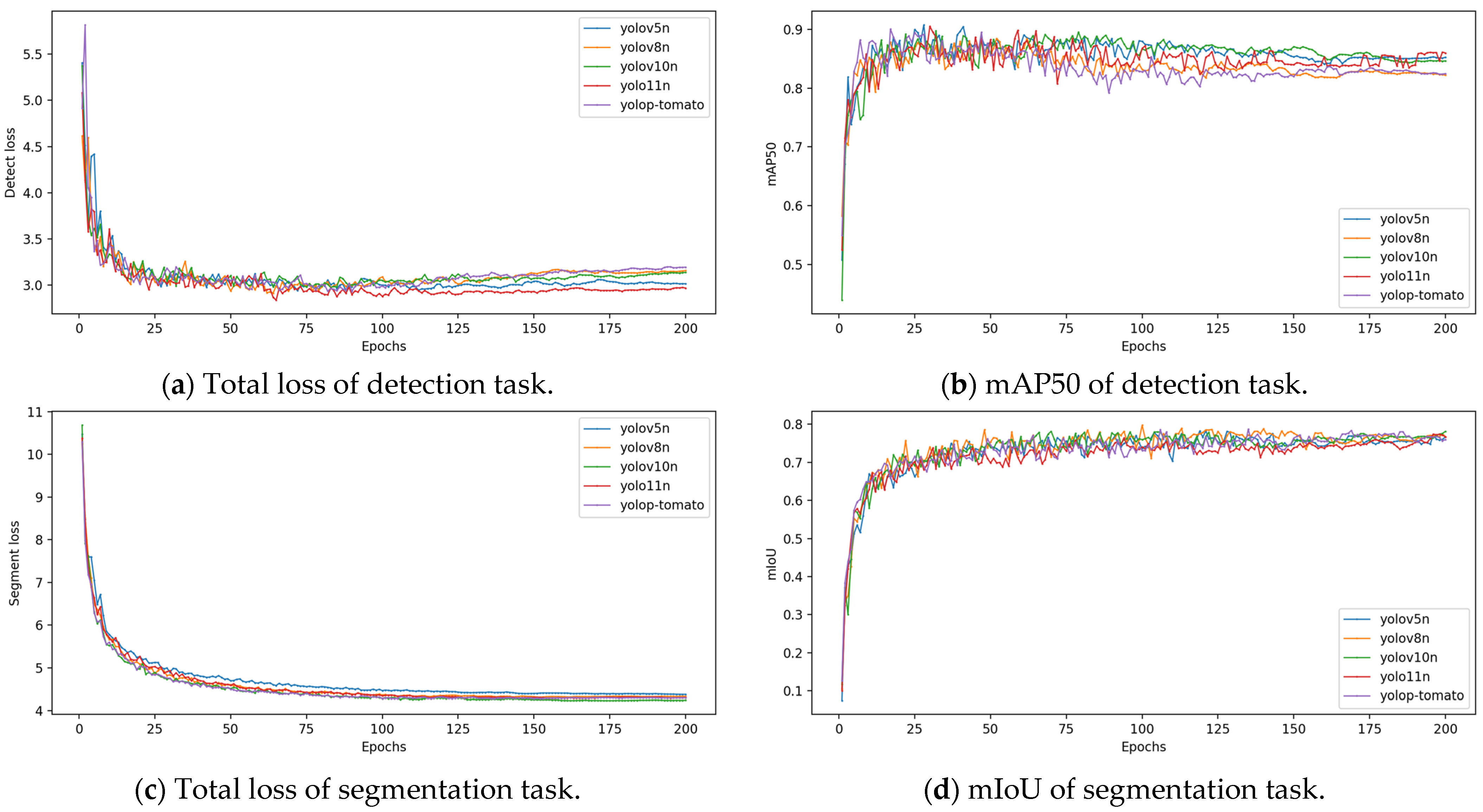
During the training phase, the validation set is employed to monitor the performance of model. The training process is illustrated in Figure 11. The tracked models encompass YOLOv5n, YOLOv8n, YOLOv10n, YOLOv11n, and the YOLO-Tomato models. Visualized metrics include loss and mAP₅₀ for detection tasks and loss and mIoU for segmentation tasks.

In terms of detection loss (a), YOLOv5n (blue) and YOLOv11n (red) generally demonstrate reduced loss on the validation set, while YOLOv8n (orange) and YOLO P-Tomato (purple) exhibit slightly elevated detection loss on the validation set. YOLOv10n (green) occupies an intermediate position. All five models demonstrate oscillatory behavior prior to 125 epochs, subsequently converging.

In the mAP₅₀ metric (b), YOLOv5n and YOLO11n also exhibited superior performance in comparison to YOLOv8n and YOLO-Tomato on the validation set. However, YOLO11n (red) exhibited persistent oscillations beyond 150 epochs, suggesting less stable validation set fitting compared to alternative models. Following 150 iterations, YOLOP-Tomato attains marginally higher validation set accuracy compared to YOLOv8n. A consideration of the performance of the test set reveals that YOLOP-Tomato achieved precision, recall, mAP₅₀, and mAP_50–95 scores of 94.9%, 85.0%, 93.6%, and 60.9%, respectively. These metrics were consistently ranked among the top performers, underscoring the model’s robust generalizability.

In the context of (c) segmentation loss, the YOLOP-Tomato model demonstrates superior performance in comparison to the YOLOv5n, YOLOv8n, YOLOv10n, and YOLO11n models on the validation set, while exhibiting a marginal edge over the YOLOv10n model. All models converge on the validation set after 150 iterations.

For the mIoU metric in (d), all models converged to similar validation set fits around 75% after 180 iterations. A consideration of the test set performance reveals that YOLOP-Tomato achieved the highest mean intersection over union (mIoU) of 77.6%, while YOLOv5n recorded the lowest at 75.7%. This further substantiates the superior accuracy of YOLOP-Tomato in segmentation tasks.

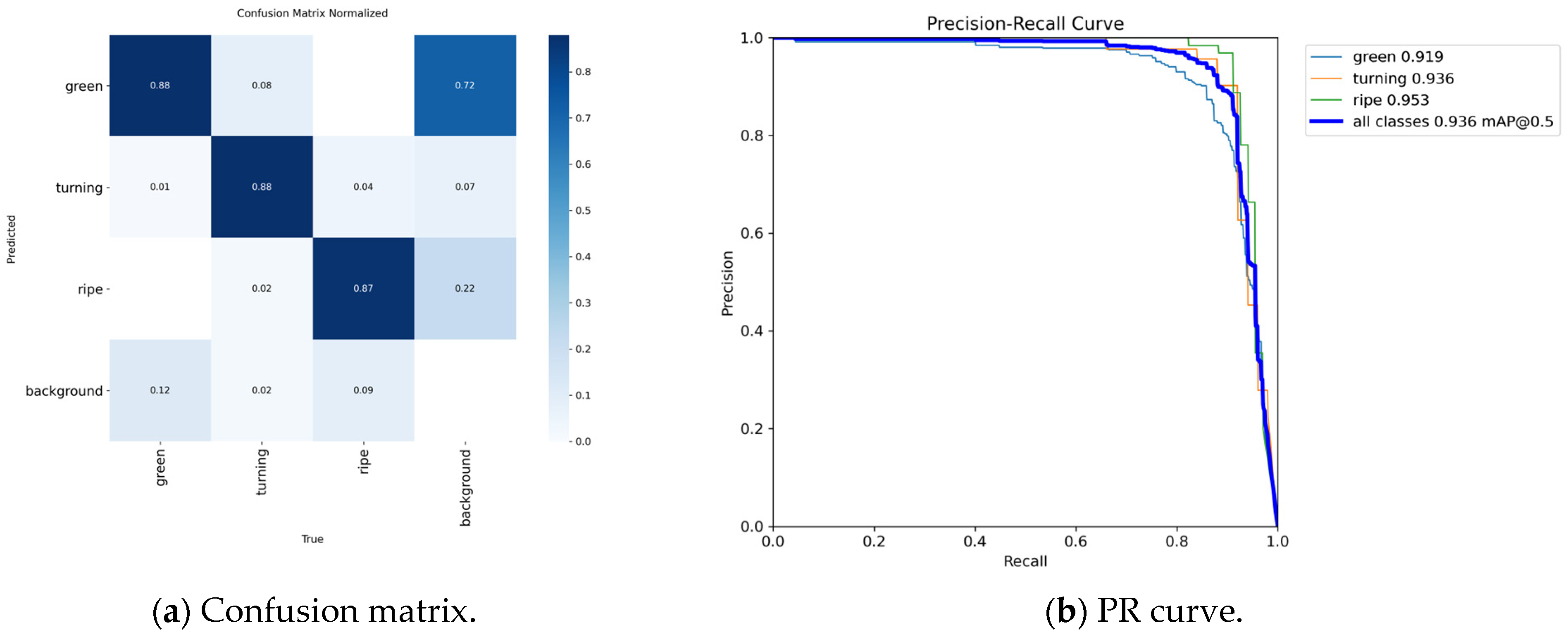
The PR curve and confusion matrix of YOLOP-Tomato are illustrated in Figure 12.

In (a), the values on the main diagonal of the matrix correspond to the accuracy rates for each category. For instance, the value of green is 0.88, indicating that 88% of true green samples were correctly classified by the model. The value of turning is also 0.88, meaning that 88% of true turning samples were correctly classified. Similarly, the value of ripe is 0.87, indicating that 87% of true ripe samples were accurately classified. The values situated off the primary diagonal in the matrix signify the misclassification rates. Among the true green samples, 1% were misclassified as turning, and 12% were misclassified as background. Among the true turning samples, 8% were misclassified as green, 2% as ripe, and 2% as background. Among true ripe samples, 4% were misclassified as turning, and 9% as background. Furthermore, the model exhibited misclassification of 46 background instances as tomatoes, indicating a misinterpretation of the data. Of these, 72% were misclassified as green tomatoes, indicating that some backgrounds resemble tomatoes, which confuses the model’s classification. The deep blue in the main diagonal region visually represents the model’s core classification capability for each category, while the lighter shades in the off-diagonal regions reflect the overall low misclassification rate.

The (b) presents the PR curves for the green, turning, ripe categories and all classes, annotated with key metrics. The PR curve plots recall on the x-axis and precision on the y-axis; its shape reflects the model’s performance under the precision–recall trade-off. For green tomatoes, the AP is 0.919. Its PR curve maintains high precision at low recall levels (recall < 0.6) before rapidly declining as recall increases. The AP for turning tomatoes is 0.936, exhibiting a trend similar to green tomatoes; the range of recall values covered within the high precision interval is slightly broader. The AP for ripe tomatoes is 0.953, the highest among the three categories, with a relatively gradual decline in precision within the high recall range. The AP values for all three classes fall between 0.919 and 0.953, indicating the model achieves high recognition accuracy across target categories.

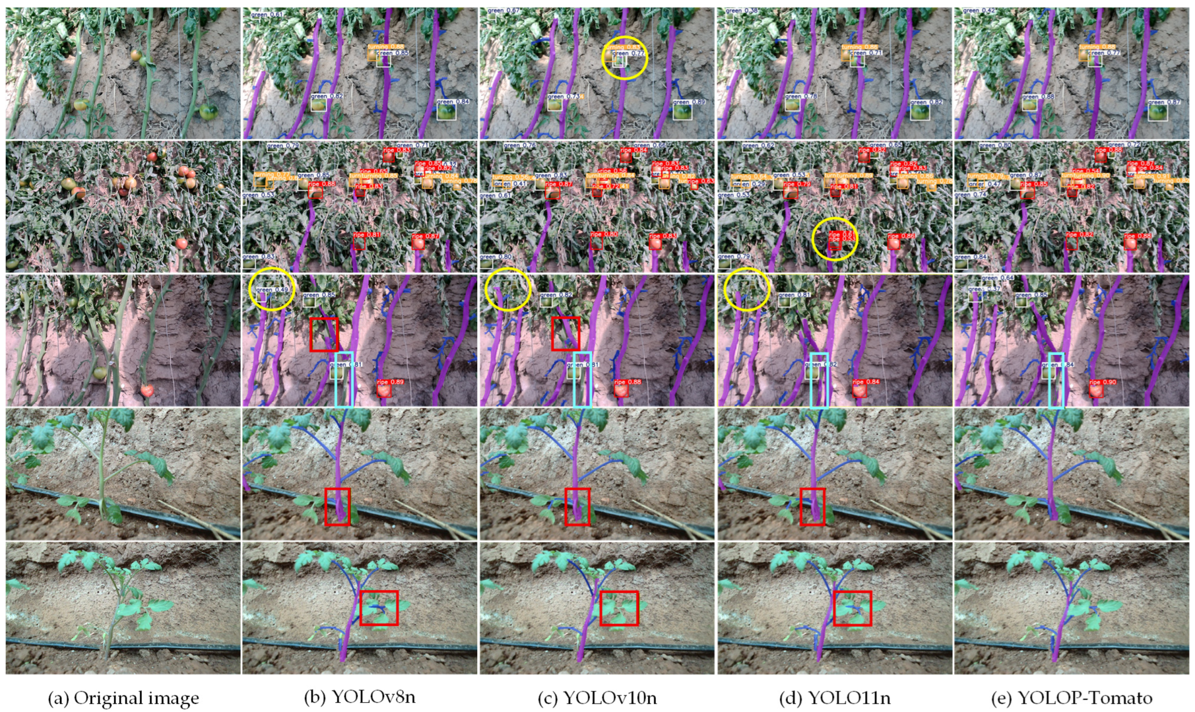
In order to present the inference results of different models on tomatoes in a more convenient and intuitive manner, the inference results on the test set are illustrated in Figure 13.

As illustrated in the image presented in the first row, the YOLOv10n model demonstrated an inability to effectively filter out the bounding box for the green tomato, consequently resulting in the generation of multiple detection boxes for a single tomato (yellow circles).

In the second row, there is a preponderance of tomatoes exhibiting more severe occlusions. The ripe tomato in the lower-middle section is partially obscured by leaves, causing its features to become less distinct. A similar failure was observed in YOLOv11n, which also failed to filter out redundant bounding boxes (yellow circles).

In the third row, the two tomatoes in the upper left corner are partially blocked by branches. The inference results from the YOLOv8n, YOLOv10n, and YOLOv11n models all exhibit varying degrees of omission (yellow circles). In the main stem segmentation below, YOLOv8n and YOLOv10n failed to complete the segmentation (red rectangle). In the lower stem segmentation, all four models exhibit varying degrees of omission (light blue rectangles). YOLOv8n and YOLOv10n almost entirely fail to segment the main stem. YOLOP-Tomato achieves superior segmentation compared to the previous two models, though it still contains some omissions. YOLO11n demonstrates the fewest omissions.

In the fourth row image, a lateral branch is observed to overlap the lower portion of the main stem. The YOLOv8n, YOLOv10n, and YOLO11n models identified this area as part of the main stem (red rectangle), while the YOLOP-Tomato model accurately identified it as a lateral branch.

In the fifth row, both YOLOv8n and YOLOv11n made incorrect classifications, labeling some leaves as lateral branches. YOLOv10n failed to detect the pixels of the lateral branch (red rectangle). YOLOP-Tomato correctly segmented the middle lateral branch.

In summary, YOLOP-Tomato exhibits robust comprehensive capabilities in tomato detection and main stem and lateral branch segmentation. The model has been demonstrated to successfully infer the ripeness of partially obscured tomatoes and perform precise segmentation of stems and branches.

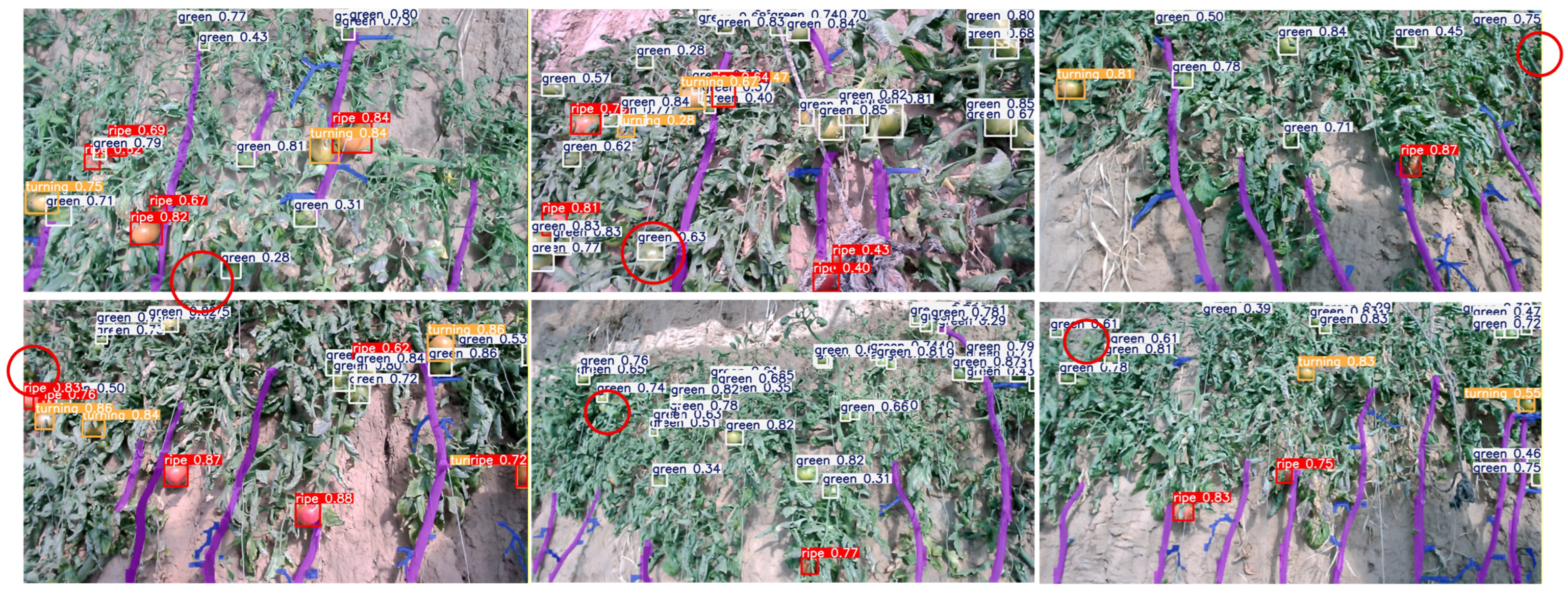
YOLOP-Tomato has certain limitations in detecting some green tomatoes, as illustrated in Figure 14.

As illustrated in the figure, YOLOP-Tomato demonstrates a propensity for false negatives in unripe green tomatoes, indicated by the red circles. The location of these tomatoes is at the image edges, with some partially obscured or having features extending beyond the pixel boundaries. In the red circle at row 1, column 2, the green tomato is obscured by a branch. While the model successfully identifies the tomato, the bounding box is smaller than the actual tomato box due to the influence of the branch. Consequently, YOLOP-Tomato experiences some limitations when detecting pixels at the image edges.

3.6. Deployment on NVIDIA Jetson AGX Orin Platform

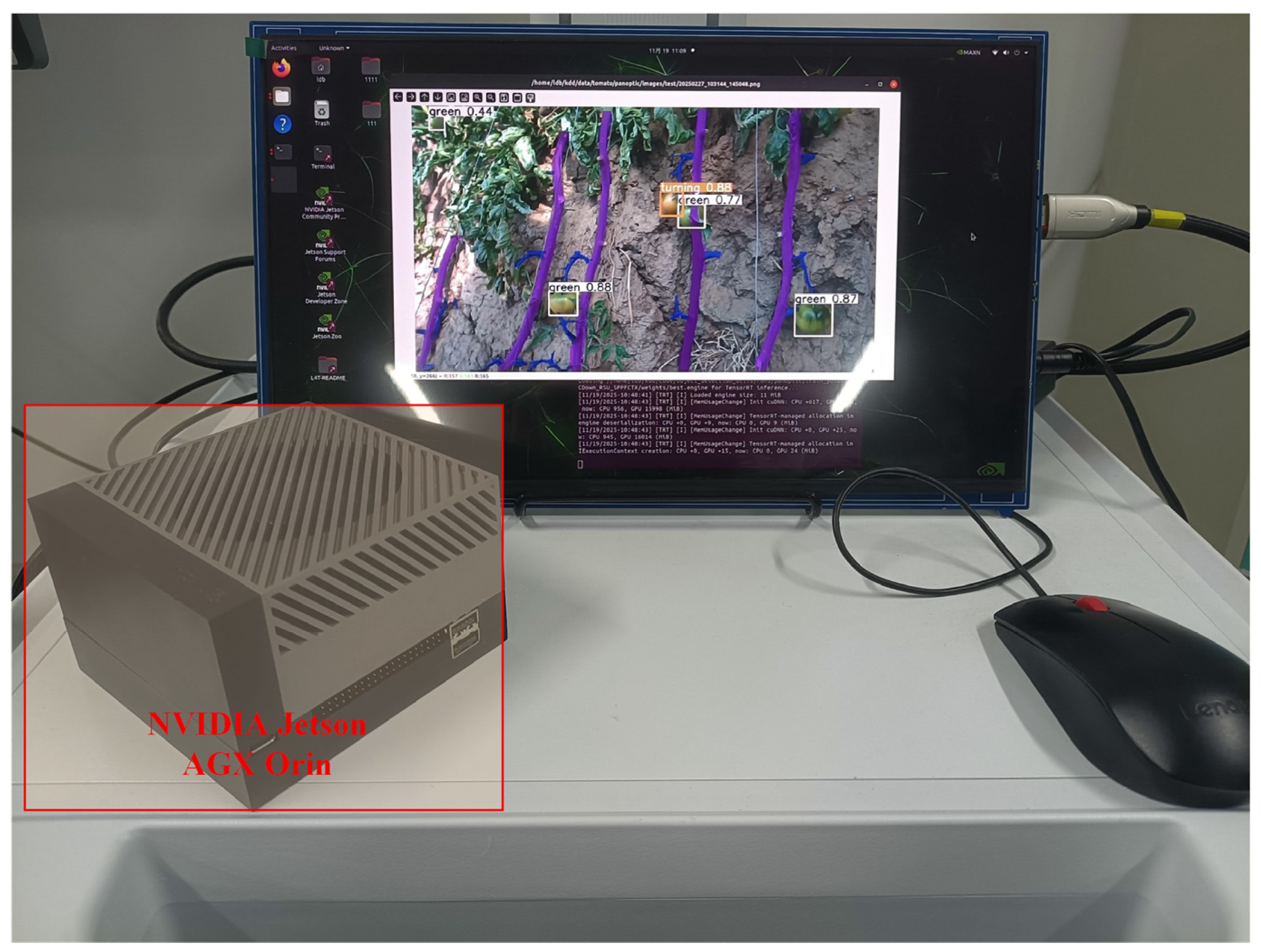
Subsequent to the training phase, the model was deployed on the NVIDIA Jetson AGX Orin (NVIDIA CORP, 2788 San Tomas Expressway, Santa Clara, CA 95051, USA) edge computing platform. This platform is an advanced high-performance AI inference system that has been demonstrated to efficiently handle model weight conversion and inference tasks in environments with limited resources. The device specifications for the NVIDIA Jetson AGX Orin are illustrated in

Table 13. Device specifications of the NVIDIA Jetson AGX Orin.

Component	Specification
CPU	12-core Arm Cortex-A78AE v8.2 64-bit CPU
GPU	NVIDIA Ampere architecture with 2048 NVIDIA CUDA cores and 64 Tensor cores
DL Accelerator	2 × NVDLA v2.0
OS	Ubuntu 20.04.6 LTS
JetPack	5.1.2-b104
Cuda	11.4
TensorRT	8.2.5.1

.

The NVIDIA Jetson AGX Orin device is illustrated in Figure 15.

With regard to the efficiency of inference processes, YOLOP-Tomato demonstrates a processing time of 5.67 ms, which is noteworthy. Employing Equation (18), the performance of YOLOP-Tomato in processing image frames on edge devices is evaluated,

$$fps={\displaystyle \frac{1000}{t_{pre}+t_{infer}+t_{post}}}$$

(18)

where $t_{pre}$ denotes preprocessing time, $t_{infer}$ denotes inference time, and $t_{post}$ denotes postprocessing time. The resulting YOLOP-Tomato achieves 20 fps when operated on the NVIDIA Jetson AGX Orin platform. This means it can process 20 frames of images per second. In summary, it meets the real-time requirements for agricultural applications.

4. Discussion

In this study, given the lightweight nature and performance advantages of the YOLOv8n model, it was adopted as the base model for enhancement, leading to the proposal of the YOLOP-Tomato model. As described in Section 2.4, the YOLOv8n backbone was augmented with three modules to enhance the model’s overall performance. Two RSU modules were incorporated at varying feature scale levels within the YOLOv8n backbone network, connecting to the decoder layer to enhance feature extraction and facilitate robust gradient flow. The SPPF module was replaced with the SPPCTX module to enhance multi-scale feature extraction. The addition of an SCDown module to the backbone was ultimately implemented as a strategy to mitigate the computational burden.

As demonstrated in Table 8, the RSU module design exhibits a greater degree of alignment with the segmentation task requirements. The RSU module employs cross-level encoding–decoding connections to enhance feature extraction in the tomato, main stem, and lateral branch regions. This direct feature encoding–decoding approach is well-suited for segmentation tasks, analogous to UNet. The mAP is constrained by both bounding box localization accuracy and category classification accuracy. Since the RSU module demonstrates greater enhancement for mIoU.

The SCDown model has been demonstrated to exert a favorable influence on both the efficacy of recall and the mIoU metrics. In contrast to conventional convolution-based downsampling techniques, SCDown employs a distinct approach by separating channel adjustment from the convolution process, thereby reducing the computational demands while maintaining the extraction of features. Furthermore, YOLOv10n employs SCDown, achieving the highest recall in Table 9. This finding indicates that SCDown exhibits a degree of preservation of tomato integrity during the process of downsampling. However, in the final YOLOP-Tomato model, the recall improvement is marginal. While the precision of the model increased by 2.5% compared to YOLOv8n, the recall only improved by 0.1%. An analysis of Table 10 indicates that YOLOP-Tomato attains recall rates of 75.8%, 88.0%, and 91.2% for green, turning, and ripe tomatoes, respectively. The presence of green tomatoes has been found to be a significant factor in the overall recall, suggesting that they do not align with the characteristics expected for this category. On the one hand, the model attains a high degree of precision by compromising some degree of accuracy. Conversely, this finding suggests that the model’s capacity to accommodate green tomatoes may be suboptimal. As illustrated in Figure 14, YOLOP-Tomato demonstrates a propensity for false negatives in the presence of green tomatoes. The presence of partial occlusions or edge-of-image placements of green tomatoes, in conjunction with the visual similarity between unripe tomatoes and background elements such as leaves, results in YOLOP-Tomato’s erroneous classification of these tomatoes as background elements. Consequently, YOLOP-Tomato encounters challenges when confronted with tomatoes in such scenarios.

Furthermore, the availability of high-quality datasets is imperative for ensuring the efficacy of the models. Given the limited size of the original dataset available in this study, a targeted strategy combining data augmentation and data expansion was employed to effectively enhance the diversity and coverage of the data distribution. By increasing the sample size and enriching the feature dimensions of the samples, this approach provided substantial data support for model training. Nevertheless, the inherent limitations of the original dataset continue to present obstacles to the enhancement of model performance. In complex real-world applications, a model’s capacity to reason about unseen novel samples is contingent entirely on the feature distribution learned from the training dataset. Consequently, expanding the scale of the original dataset and optimizing the rationality of its distribution to better align with actual tomato growth scenarios in greenhouse environments will become critical issues requiring urgent attention in future research.

A thorough analysis of inference speed and fps of YOLOP-Tomato reveals that it achieves an inference speed of 5.67 ms, thereby maintaining exceptionally fast processing overall. However, the overall fps is 20. Preliminary analysis suggests that the mean postprocessing duration is 49.96 ms. This is attributable to the augmented computational overhead resulting from the concurrent execution of detection and segmentation operations. Subsequent research endeavors will center on the multi-task decoupling module, with the objective of enhancing the model’s processing speed of image frames.

5. Conclusions

This study proposes YOLOP-Tomato, a multi-task panoramic detection and seg-mentation model based on the YOLOv8n architecture. A connection of feature channels between the backbone and head is established by two RSU modules. The SPPF module is replaced with SPPCTX to extract rich multi-scale contextual features. Furthermore, two SCDown modules replaced the original convolutional modules in the final two layers of the backbone. The YOLOP-Tomato has been demonstrated to achieve significant improvements in precision, recall, mAP₅₀, mAP_50–95, and mIoU of 94.9%, 85.0%, 93.6%, 60.9%, and 77.6%. These results represent improvements of 2.5%, 0.1%, 0.5%, 1.1%, and 1.4% over YOLOv8n. When deployed on an NVIDIA Jetson AGX Orin device, the model achieves an inference speed of 5.67 ms and 20 fps, delivering competitive overall performance.

Within the multi-task learning framework of the YOLOP-Tomato model, the outputs for the detection and segmentation tasks remain independent computational processes. The core operations within the output heads continue to demonstrate decoupled redundancy, resulting in an inability to achieve synchronized output or effective integration of core operations. This suggests the presence of opportunities for enhancement with respect to the synergistic optimization of model performance and efficiency. Subsequent research endeavors will concentrate on lightweight fusion designs for multi-task output heads, with the objective of reducing redundant computations between tasks to enable efficient, coordinated output of multi-task results.

Furthermore, the YOLO series is undergoing continuous refinement and development. According to reports, YOLO26 is scheduled for official release in 2026 [31]. The initial YOLO version, designated as such due to its association with a specific year, prioritizes the fulfillment of high-performance inference demands for mobile and edge computing devices that are currently under development. In alignment with prevailing trends in edge AI detection and deployment requirements in agricultural contexts, the introduction of YOLO26 is set to spearhead research on lightweight edge models, thereby providing more efficient technical support for on-device deployment in agricultural scenarios such as greenhouse tomato detection. Subsequent research endeavors may benefit from leveraging YOLO26’s fundamental architectural design to enhance the integration of multi-task detection and segmentation, investigate model lightweighting and inference acceleration methodologies that are more appropriate for agricultural edge scenarios, and facilitate the large-scale implementation of intelligent detection technologies in agricultural production.

References

1. Food and Agriculture Organization of the United Nations. Production/Crops and Livestock Products. Available online: https://www.fao.org/faostat/en/#data/QCL (accessed on 6 October 2025).
2. Kamilaris, A.; Prenafeta-Boldú, F.X. Deep learning in agriculture: A survey. Comput. Electron. Agric. 2018, 147, 70–90. [Google Scholar] [CrossRef] [Scilit]
3. Gu, W.; Liu, H.; Wei, J.; Gao, W.; Yin, Y.; Liu, X. Tomato Fruit Recognition in Complex Scenes Based on FPBW-YOLO v8. Trans. Chin. Soc. Agric. Mach. 2025, 56, 467–478. [Google Scholar] [CrossRef]
4. Wang, X.; Tang, C.; Zhu, J.; Guo, C.; Liu, Y.; Wang, S. Tomato Cluster Ripeness Recognition at Night Based on Depth Enhancement and Feature Noise Reduction. Trans. Chin. Soc. Agric. Mach. 2025, 56, 363–374. [Google Scholar] [CrossRef]
5. Liang, X.; Wei, Z.; Chen, K. A method for segmentation and localization of tomato lateral pruning points in complex environments based on improved YOLOV5. Comput. Electron. Agric. 2025, 229, 109731. [Google Scholar] [CrossRef] [Scilit]
6. Zhang, Y.; Yang, Q. A Survey on Multi-Task Learning. arXiv 2017, arXiv:1707.08114. [Google Scholar] [CrossRef] [Scilit]
7. Chen, W.; Liu, M.; Zhao, C.; Li, X.; Wang, Y. MTD-YOLO: Multi-task deep convolutional neural network for cherry tomato fruit bunch maturity detection. Comput. Electron. Agric. 2024, 216, 108533. [Google Scholar] [CrossRef] [Scilit]
8. Li, J.; Gong, G.; Zhang, J.; Liu, X.; Jiang, S.; Wu, X.; Xie, H.; Gu, L. Multi-task learning based approach for potato edibility detection and defect segmentation. J. Food Compos. Anal. 2025, 148, 108420. [Google Scholar] [CrossRef] [Scilit]
9. Wu, M.; Lin, H.; Shi, X.; Zhu, S.; Zheng, B. MTS-YOLO: A Multi-Task Lightweight and Efficient Model for Tomato Fruit Bunch Maturity and Stem Detection. Horticulturae 2024, 10, 1006. [Google Scholar] [CrossRef] [Scilit]
10. Qin, X.; Cao, J.; Zhang, Y.; Dong, T.; Cao, H. Development of an Optimized YOLO-PP-Based Cherry Tomato Detection System for Autonomous Precision Harvesting. Processes 2025, 13, 353. [Google Scholar] [CrossRef] [Scilit]
11. Rong, J.; Li, X.; Zheng, W.; Chen, T.; Yuan, T.; Wang, P.; Li, W. An end-to-end maturity prediction and hierarchical counting method for cherry tomatoes. Biosyst. Eng. 2025, 256, 104191. [Google Scholar] [CrossRef] [Scilit]
12. Mittal, S. A Survey on optimized implementation of deep learning models on the NVIDIA Jetson platform. J. Syst. Archit. 2019, 97, 428–442. [Google Scholar] [CrossRef] [Scilit]
13. Zhou, Y.; Yang, K. Exploring TensorRT to Improve Real-Time Inference for Deep Learning. In Proceedings of the 2022 IEEE 24th International Conference on High Performance Computing & Communications, Chengdu, China, 18–20 December 2022; pp. 2011–2018. [Google Scholar] [CrossRef] [Scilit]
14. Wu, X.; Dong, Z.; Wang, C.; Zhu, Z.; Guo, Y.; Zheng, S. ESG-YOLO: An Efficient Object Detection Algorithm for Transplant Quality Assessment of Field-Grown Tomato Seedlings Based on YOLOv8n. Agronomy 2025, 15, 2088. [Google Scholar] [CrossRef] [Scilit]
15. Weng, W.; Lai, Z.; Cui, Z.; Chen, Z.; Chen, H.; Lin, T.; Wang, J.; Zheng, S.; Chen, G. GCD-YOLO: A deep learning network for accurate tomato fruit stalks identification in unstructured environments. Smart Agric. Technol. 2025, 12, 101465. [Google Scholar] [CrossRef] [Scilit]
16. Cao, L.; Chen, Y.; Jin, Q. Lightweight Strawberry Instance Segmentation on Low-Power Devices for Picking Robots. Electronics 2023, 12, 3145. [Google Scholar] [CrossRef] [Scilit]
17. Ma, S.; Lu, X.; Zhang, L. TSINet: A Semantic and Instance Segmentation Network for 3D Tomato Plant Point Clouds. Appl. Sci. 2025, 15, 8406. [Google Scholar] [CrossRef] [Scilit]
18. Ullah, R.; Ali, W.; Ghanni, U. Deep Reinforcement Learning for Robust USVs Navigation in Diverse Environmental Scenarios. Int. J. Data Inform. Intell. Comput. 2025, 4, 1–10. [Google Scholar] [CrossRef] [Scilit]
19. Nisha, C.M.; Thangarasu, N. Deep Learning Algorithms and Their Relevance: A Review. Int. J. Data Inform. Intell. Comput. 2023, 2, 1–10. [Google Scholar] [CrossRef] [Scilit]
20. Wu, Q.; Huang, H.; Song, D.; Zhou, J. YOLO-PGC: A Tomato Maturity Detection Algorithm Based on Improved YOLOv11. Appl. Sci. 2025, 15, 5000. [Google Scholar] [CrossRef] [Scilit]
21. Qin, X.; Zhang, Z.; Huang, C.; Dehghan, M.; Zaiane, O.; Jagersand, M. U2-Net: Going Deeper with Nested U-Structure for Salient Object Detection. Pattern Recognit. 2020, 106, 107404. [Google Scholar] [CrossRef] [Scilit]
22. He, K.; Zhang, X.; Ren, S.; Sun, J. Spatial Pyramid Pooling in Deep Convolutional Networks for Visual Recognition. IEEE Trans. Pattern Anal. Mach. Intell. 2015, 37, 1904–1916. [Google Scholar] [CrossRef] [Scilit] [PubMed]
23. Vaswani, A.; Shazeer, N.; Parmar, N.; Uszkoreit, J.; Jones, L.; Gomez, A.N.; Kaiser, Ł.; Polosukhin, I. Attention Is All You Need. In Proceedings of the 31st International Conference on Neural Information Processing Systems (NIPS’17), Long Beach, CA, USA, 4–9 December 2017; pp. 6000–6010. [Google Scholar]
24. Yu, F.; Koltun, V. Multi-Scale Context Aggregation by Dilated Convolutions. In Proceedings of the International Conference on Learning Representations (ICLR 2016), San Juan, PR, USA, 2–4 May 2016. [Google Scholar]
25. Wang, A.; Chen, H.; Liu, L.; Chen, K.; Lin, Z.; Han, J.; Ding, G. YOLOv10: Real-Time End-to-End Object Detection. Adv. Neural Inf. Process. Syst. 2024, 37, 107984–108011. [Google Scholar] [CrossRef] [Scilit]
26. Ren, S.; He, K.; Girshick, R.; Sun, J. Faster R-CNN: Towards Real-Time Object Detection with Region Proposal Networks. IEEE Trans. Pattern Anal. Mach. Intell. 2017, 39, 1137–1149. [Google Scholar] [CrossRef] [Scilit] [PubMed]
27. Liu, W.; Anguelov, D.; Erhan, D.; Szegedy, C.; Reed, S.; Fu, C.; Berg, A.C. SSD: Single Shot MultiBox Detector. In Proceedings of the European Conference on Computer Vision, Amsterdam, The Netherlands, 11–14 October 2016; pp. 21–37. [Google Scholar] [CrossRef] [Scilit]
28. Zhao, Y.; Lv, W.; Xu, S.; Wei, J.; Wang, G.; Dang, Q.; Liu, Y.; Chen, J. DETRs Beat YOLOs on Real-time Object Detection. In Proceedings of the 2024 IEEE/CVF Conference on Computer Vision and Pattern Recognition (CVPR), Seattle, WA, USA, 16–22 June 2024; pp. 16965–16974. [Google Scholar] [CrossRef] [Scilit]
29. Jocher, G. YOLOv5 by Ultralytics, Version 7.0. 2020. Available online: https://github.com/ultralytics/yolov5 (accessed on 19 August 2025).
30. Jocher, G.; Qiu, J.; Chaurasia, A. Ultralytics YOLO (Version 8.0.0). 2023. Available online: https://github.com/ultralytics/ultralytics (accessed on 19 August 2025).
31. Ultralytics YOLO26. Available online: https://docs.ultralytics.com/zh/models/yolo26/ (accessed on 22 December 2025).
Figure 1. Data acquisition equipment.
Agronomy 16 00150 g001
Figure 2. Tomato data.
Agronomy 16 00150 g002
Figure 3. Tomato detection, main stem, and lateral branch segmentation annotation. (a) represents the annotation of tomato detection, which uses bounding boxes to mark the pixel locations of tomatoes. The color of the box indicates the stage of ripeness of the tomato: green for the green stage, yellow for the turning stage, and red for the ripe stage. (b,c) represent main stem and lateral branch annotations.
Agronomy 16 00150 g003
Figure 4. Data augmentation. Rows (1) to (4) represent collection of fruit data from tomatoes of different ripeness. These tomatoes were situated in different distances, angles, and lighting conditions. Some tomato fruits exhibit partial occlusion, and stem and branch data are also included. (5) represents supplementary stem data collected during the early growth stage of tomatoes. (a) represents the original image, (b) represents flip enhancement, (c) represents rotation enhancement, (d) represents brightness variation, and (e) represents Gaussian blur and noise.
Agronomy 16 00150 g004
Figure 5. Visualization of data dictionary. The two tomatoes used for detection are marked with green and yellow boxes, the two main stems used for segmentation are marked with red and dark blue polygons, and the three lateral branches are marked with light green, pink and brown polygons respectively. The polygons are surrounded by dots, and the data dictionary on the right represents the labels of the instances, distinguishing each corresponding instance by color.
Agronomy 16 00150 g005
Figure 6. The structure of YOLOP-Tomato.
Agronomy 16 00150 g006
Figure 7. The structure of RSU.
Agronomy 16 00150 g007
Figure 8. The structure of SPPCTX.
Agronomy 16 00150 g008
Figure 9. The structure of SCDown.
Agronomy 16 00150 g009
Figure 10. Data distribution. Row (1) displays the original training set, row (2) presents the training set that was expanded using Strategy 1, and row (3) shows the training set that was expanded using Strategy 2. The bar chart (a) displays the number of tomato classes. Green, orange, and red represent green, turning, and ripe tomatoes, respectively. (b) represents scatter plot of the height and width distributions of bounding boxes. (c) represents box plots of the RGB channel distributions for tomatoes, where the first three columns (red, green, blue box plots) represent the RGB channels for the green tomato, the middle three columns (red, green, blue box plots) represent the RGB channels for the turning tomato, and the last three columns (red, green, blue box plots) represent the RGB channels for the ripe tomato. (d) is a bar chart of segmentation instance counts, with dark blue representing the main stem and light blue representing lateral branches. (e) is a scatter plot of height and width distributions for segmentation bounding boxes.
Agronomy 16 00150 g010
Figure 11. Visualization of the training process.
Agronomy 16 00150 g011
Figure 12. Visualization of the test results.
Agronomy 16 00150 g012
Figure 13. Visualization of inference results from different models. (a) represents the original image, (b) represents the YOLOv8n inference image, (c) represents the YOLOv10n inference image, (d) represents the YOLO11n inference image, and (e) represents the YOLOP-Tomato inference image. Detection boxes are used to annotate tomatoes and their ripeness: green is annotated with white boxes, turning is annotated with orange boxes, and ripe is annotated with red boxes. The main stem is annotated in purple, and lateral branches are annotated in blue. Yellow circles indicate tomatoes that were missed or duplicated, while red and blue rectangles include incorrect or omitted segmentation instances.
Agronomy 16 00150 g013
Figure 14. The limitation of YOLOP-Tomato. The red coil included tomatoes that had been missed during testing.
Agronomy 16 00150 g014
Figure 15. NVIDIA Jetson AGX Orin.
Agronomy 16 00150 g015