HSDT-TabNet: A Dual-Path Deep Learning Model for Severity Grading of Soybean Frogeye Leaf Spot

Abstract

Soybean frogeye leaf spot (FLS), a serious soybean disease, causes severe yield losses in the largest production regions of China. However, both conventional field monitoring and machine learning algorithms remain challenged in achieving rapid and accurate detection. In this study, an HSDT-TabNet model was proposed for the grading of soybean FLS under field conditions by analyzing unmanned aerial vehicle (UAV)-based hyperspectral data. This model employs a dual-path parallel feature extraction strategy: the TabNet path performs sparse feature selection to capture fine-grained local discriminative information, while the hierarchical soft decision tree (HSDT) path models global nonlinear relationships across hyperspectral bands. The features from both paths are then dynamically fused via a multi-head attention mechanism to integrate complementary information. Furthermore, the overall generalization ability of the model is improved through hyperparameter optimization based on the tree-structured Parzen estimator (TPE). Experimental results show that HSDT-TabNet achieved a macro-accuracy of 96.37% under five-fold cross-validation. It outperformed the TabTransformer and SVM baselines by 2.08% and 2.23%, respectively. For high-severity cases (Level 4–5), the classification accuracy exceeded 97%. This study provides an effective method for precise field-scale crop disease monitoring.

1. Introduction

Soybean (Glycine max L.) is a globally significant crop for food, oil production, and industrial raw materials [1]. However, with expanding cultivation areas and the impacts of global climate change, soybean diseases are occurring more frequently and with higher severity, posing a significant threat to yield and quality [2]. Taking Heilongjiang Province, China’s largest soybean-growing region, as an example, its distinctive cold–temperate monsoon climate creates ideal conditions for the growth and dissemination of multiple pathogens. Notably, frogeye leaf spot (FLS) caused by Cercospora sojina Hara is particularly prominent. This disease can lead to extensive necrosis of leaves and reduced photosynthetic capacity, and in severe cases, it can infect pods and seeds, causing yield losses of over 60% [3]. Therefore, developing efficient and accurate soybean disease detection and grading technologies is not only vital for national food security but also provides key support for sustainable agricultural development.

Traditional field diagnosis of diseases primarily relies on manual visual inspection or laboratory-based chemical assays [4]. However, manual surveys suffer from subjectivity, low accuracy, and high labor demands; while chemical assays provide precision, they require destructive sampling and expensive equipment, making them unsuitable for large-scale, rapid, and non-destructive monitoring. These limitations highlight the urgent need to improve field disease detection methods.

Recently, in controlled greenhouse or laboratory environments, numerous studies have demonstrated that integrating RGB or hyperspectral imaging (HSI) with artificial intelligence (AI) algorithms can achieve high-accuracy disease classification [5]. For example, Alves et al. [6] captured RGB images of leaves exhibiting different severity levels across five species under controlled lighting and homogeneous backgrounds, calculated ten spectral indices, and developed a boosted regression tree model, achieving over 97% accuracy in disease severity prediction. Zhang et al. [7] used a spectral imaging setup to scan strawberry leaves 24 h post-inoculation with frogeye leaf spot and anthracnose, employed CARS and ReliefF for spectral fingerprint and vegetation index extraction, and classified with BPNN, SVM, and RF, reaching fusion accuracies of 97.78%, 94.44%, and 93.33%, respectively. Feng et al. [8] proposed the DC²Net—a network combining deformable and dilated convolutions—for greenhouse detection of Asian soybean rust, attaining 96.73% overall accuracy. However, the significant differences between controlled laboratory environments and real field conditions limit the applicability of these methods in open-field settings.

To facilitate crop disease surveillance in true open-field environments, RGB-equipped unmanned aerial vehicle (UAV) platforms combined with deep learning have attracted considerable attention. For example, Amarasingam et al. [9] utilized UAV-acquired RGB imagery to detect sugarcane white leaf disease (WLD) and compared multiple detection models, including YOLOv5, YOLOR, DETR, and Faster R-CNN. YOLOv5 achieved the best performance, with mAP@0.50 and mAP@0.95 of 93% and 79%, respectively. Deng et al. [10] employed ultra-high-resolution RGB UAV images along with the DeepLabv3+ semantic segmentation network to identify wheat stripe rust under field conditions, achieving an F1-score of 81%, thus demonstrating the potential for large-scale disease monitoring.

RGB imaging offers several advantages, including lower cost, high spatial resolution, ease of operation, and real-time processing capabilities. However, its limitations—especially under field conditions—include sensitivity to lighting fluctuations, atmospheric disturbances, and sensor noise, particularly when UAVs operate at lower altitudes and slower speeds to ensure adequate spatial resolution [11,12]. Castelão et al. [13] found that soybean foliar disease classification accuracy peaked at 98.34% when flying at 1–2 m, but it dropped by approximately 2% for every 1 m increase in altitude, illustrating the trade-off between spatial resolution and acquisition efficiency. Despite the availability of high-resolution RGB cameras that can capture quality images at higher speeds and altitudes, performance may still degrade due to reduced spatial detail and increased environmental interference.

To address these challenges, recent research has increasingly explored UAV-based hyperspectral imaging (HSI) for non-destructive, field-scale disease monitoring. Unlike RGB images, hyperspectral data, although more costly, provide rich spectral information across a wide range of wavelengths, offering the ability to detect subtle physiological changes—such as variations in chlorophyll content, water stress, or structural alterations—prior to the emergence of visible symptoms [14,15]. Additionally, HSI can reduce the influence of external noise caused by lighting and atmospheric variations, enabling disease detection at higher altitudes with consistent accuracy. However, due to its line-scan imaging mechanism, it requires slower flight speeds, and for both HSI and RGB sensors, higher altitudes reduce spatial resolution and increase sensitivity to atmospheric and lighting conditions [16]. Abdulridha et al. [17] applied UAV-based hyperspectral imaging on 960 wheat plots and used 14 spectral vegetation indices along with machine learning methods such as QDA, RF, decision tree, and SVM. RF achieved 85% classification accuracy across four severity levels, with binary classification reaching 88%. In another study, Li et al. [18] assessed cotton disease severity using wavelet features and vegetation indices, achieving an R² of 0.9007 and RMSE of 6.0887 through GA/PSO/GWO-optimized SVM models. Zeng et al. [19] detected powdery mildew in rubber trees using a low-altitude UAV-HSI system and a multi-scale attention CNN, achieving a maximum Kappa coefficient of 98.04%. Currently, few studies have quantitatively assessed soybean disease severity using UAV-based HSI. Meng et al. [20] combined multispectral UAV data with random forest regression to dynamically monitor bacterial blight in soybean via CCI and GNDVI. In summary, UAV-based hyperspectral imaging provides superior spectral sensitivity, enabling the detection of subtle physiological changes and early disease symptoms that are often not discernible through conventional imaging. Although its line-scan acquisition mechanism typically necessitates slower flight speeds, hyperspectral systems maintain diagnostic stability under variable environmental conditions and higher flight altitudes, offering significant advantages for precision disease monitoring.

However, traditional machine learning methods such as SVM [21] and RF [22] rely on manual feature engineering, making it difficult to fully exploit the complex information inherent in hyperspectral data, and their generalization ability is limited. Existing deep learning architectures, such as CNNs, are primarily designed for two-dimensional images and require large datasets for training, making them unsuitable for directly handling high-dimensional tabular hyperspectral reflectance data [23]. How to design efficient end-to-end deep learning models specifically for small-sample, high-dimensional hyperspectral tabular data remains an open challenge.

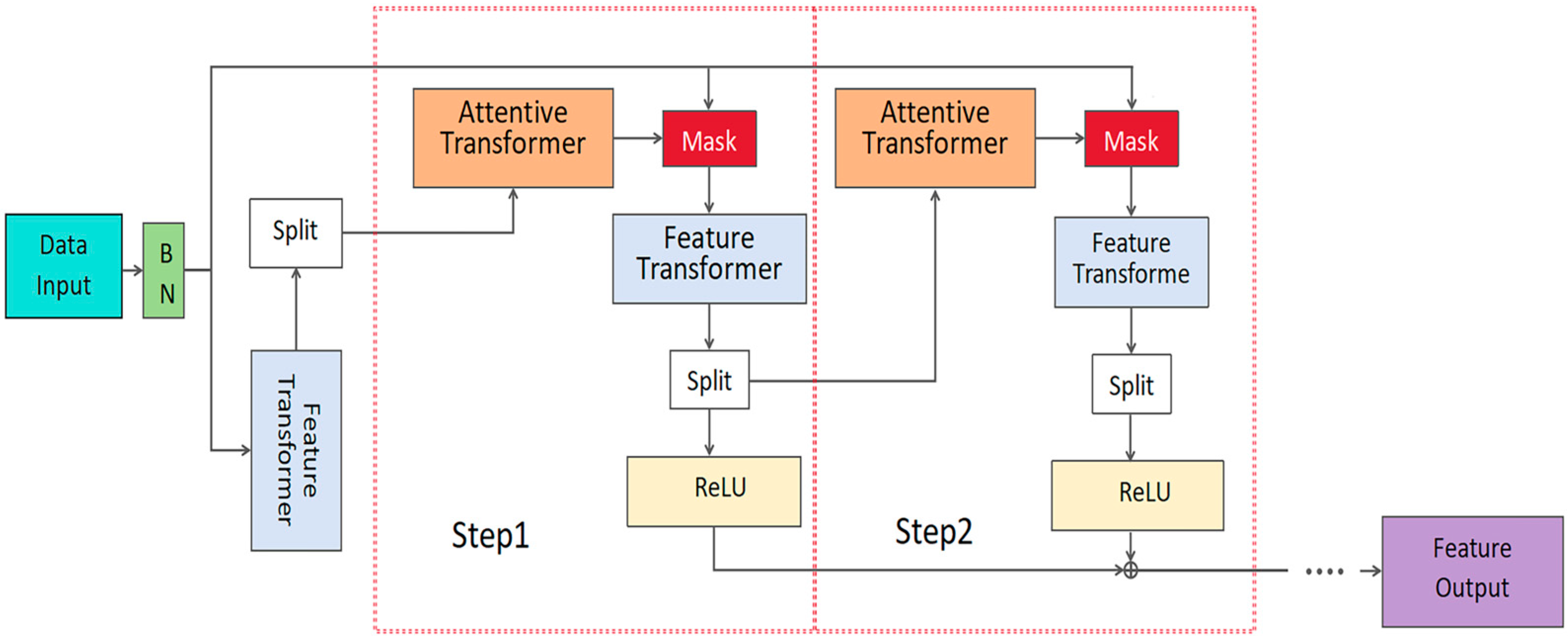
To address the above-mentioned challenges, we propose a novel dual-path deep learning framework—HSDT-TabNet. The TabNet path emphasizes sparse local feature selection, while the HSDT path captures hierarchical global interactions. These complementary features are dynamically fused via a multi-head attention mechanism. Furthermore, to enhance robustness and performance, the model employs tree-structured Parzen estimator (TPE) optimization for hyperparameter tuning. This work introduces a tabular deep learning model, providing a practical solution for field-based soybean disease grading.

2. Materials and Methods

2.1. Study Area and Experimental Materials

The UAV observation site for soybean FLS was located at the Xiangyang Research Base of Northeast Agricultural University (126.93° E, 45.76° N), where the cultivar Dongnong 109 (Northeast Agricultural University, China) was sown at a row spacing of 0.5 m and plant spacing of 0.1 m. The trial field comprised five gradations of disease severity, each with three replicates, yielding 15 plots of 10 m × 10 m (Figure 1).

The disease severity was controlled by varying the number of inoculations with the FLS pathogen. Using the standard FLS isolate from the College of Agronomy of Northeast Agricultural University, a conidial suspension (1.0 × 10⁵ mL⁻¹) was formulated with 3% sucrose to improve spore attachment, producing the inoculation solution. According to national standards, the FLS inoculation solution was inoculated in the early flowering stage (R1 stage) of soybeans under cloudy conditions in the evening. Gradient 1 was not inoculated with the pathogen as a healthy control, while gradients 2 to 5 were inoculated with the pathogen 1 to 4 times, with an interval of 24 h between each inoculation.

Disease severity grading for each experimental plot was determined through continuous in-field assessment by a team of agronomy experts, following the national standard “Technical Specification for Identification of Soybean Frogeye Leaf Spot” (DB-23/T 3111–2022) (

Table 1. Grading standard for soybean FLS.

Disease Grade	Grading Standards
0	No disease spots
1	Less than 1% of the lesion area
2	Disease spot area 1–5%
3	Disease spots occupy 6–20% of leaf area
4	Disease spots occupy 21–50% of the leaf area
5	Disease spots account for over 51% of the leaf area

). The expert team tracked and confirmed that each plot maintained a uniform disease grade across its entire area prior to UAV data acquisition. This rigorous ground-truth validation ensured that the UAV-based hyperspectral imagery could be reliably associated with accurate disease severity labels. Ultimately, these data were integrated to construct a comprehensive spatiotemporal soybean frogeye leaf spot dataset.

2.2. Data Acquisition and Preprocessing

2.2.1. UAV-Based Hyperspectral Imaging Acquisition System

The UAV remote-sensing platform used in this study consists of a DJI Matrice 300 RTK drone (DJI, Shenzhen, China), a three-axis stabilized gimbal, and a ground control station (

Table 2. Technical parameters of UAV.

Technical Parameters of UAV
Maximum takeoff weight	9 kg
Maximum single battery life	55 min
Maximum tolerable wind speed	12 m/s

).

The mounted hyperspectral imaging system consists of a Cubert S185 airborne imaging spectrometer (Cubert GmbH, Ulm, Germany) and an ultra-compact computing unit; the hyperspectral sensor’s technical specifications are presented in

Table 3. Technical parameters of the hyperspectral sensor.

Technical Parameters of Hyperspectral Sensor
Spectral coverage range	450~950 nm
Spectral sampling interval	4 nm
Number of channels	126
Single hyperspectral cube acquisition time	0.001 s

.

In addition, the UAV’s integrated position and orientation system (POS) can record the geographic coordinates of the imagery in real time, ensuring spatial accuracy of the data.

2.2.2. Collection and Stitching of HSI

UAV-based hyperspectral data were collected on five occasions at 0, 5, 10, 15, and 20 days post-inoculation. Each acquisition occurred between 10:00 and 12:00 to directly capture ortho-corrected hyperspectral imagery of the entire experimental area, minimizing the effects of illumination and wind. Flights were conducted under clear, cloudless skies with wind speeds below Beaufort 5 and a maximum duration of 40 min. Prior to takeoff, a standard white reference calibration panel (Spectralon, Labsphere Inc., Sutton, NH, USA) was placed in the experimental field to perform radiometric calibration, ensuring the conversion of raw sensor data to accurate reflectance values. White-reference and dark-current calibrations were also performed on the sensor before each flight. Flight overlap was set to 75% lateral and 90% longitudinal at an altitude of 50 m, yielding a spatial resolution of 3.0 cm.

The UAV hyperspectral platform acquired multiple single-scene images that required mosaicking. First, the raw data were converted to reflectance images using the spectrometer’s native Cube-Pilot 1.5.5 software. Next, the panchromatic image and its corresponding POS data were imported into Agisoft PhotoScan 1.5.0, where POS coordinates and tie-point matching between adjacent images were used to generate a 3D point cloud. Finally, the panchromatic and hyperspectral data cubes were fused and ortho-corrected to produce georeferenced UAV hyperspectral imagery.

2.2.3. Data Preprocessing

ENVI 5.3 (Exelis Visual Information Solutions, Boulder, CO, USA) was used for geometric rectification of the hyperspectral data, ensuring full coverage of all 15 plots. To minimize external interference, we first excluded the edge areas of each experimental subplot. We then overlaid a 3 × 3 grid on the remaining interior area and randomly selected two non-overlapping 30 × 30 pixel (0.9 m × 0.9 m) regions of interest (ROIs) within each grid cell, yielding 18 ROIs per subplot.

Raw spectra extracted from the ROIs underwent outlier detection and removal to eliminate aberrant values due to sensor noise and environmental interference. Spectral curves were smoothed using a Savitzky–Golay filter (window length = 11, polynomial order = 2) to reduce high-frequency noise while preserving salient features. The smoothed spectra were subjected to Z-score normalization to enhance data consistency and comparability. The original dataset was imbalanced (702, 216, 216, 108, 54, and 54 samples for Grades 0 to 5, respectively). To balance the class distribution, SMOTE oversampling and downsampling were applied, resulting in 216 samples per disease level.

To validate the biophysical basis of our model’s discriminative capability, we analyzed the spectral reflectance patterns across disease severity levels. Figure 2 shows the average spectral curves for healthy (Grade 0) and diseased (Grades 1–5) soybean samples across 450–950 nm.

These systematic spectral variation patterns clearly reveal the impact of diseases on the physiological and biochemical characteristics and optical properties of soybean leaves, which constitute the key physical basis for our model to effectively distinguish different severity levels.

2.3. The Proposed HSDT-TabNet Model

The dataset in this study is characterized by a small sample size, high dimensionality, and strong inter-band correlations, which place stringent demands on the performance of conventional modeling approaches. To address these challenges, we propose HSDT-TabNet, a dual-path feature-extraction architecture that integrates local and global modeling capabilities to enhance both the feature learning capacity and generalization of hyperspectral data in disease-recognition tasks.

TabNet, a deep neural network specifically designed for structured tabular data [24], employs multi-step interleaved stacks of Feature Transformer and Attentive Transformer modules to iteratively filter and transform the input features, thereby strengthening the model’s ability to capture fine-grained local information—making it particularly well-suited for feature compression and information retention in high-dimensional, small-sample contexts.

In contrast, the hierarchical soft decision tree (HSDT) focuses on global structural modeling [25]. Its internal nodes use soft split nodes to probabilistically partition data, alleviating the limitations of traditional hard-split decision trees when handling fuzzy feature boundaries. The multilayer architecture of HSDT facilitates hierarchical information flow, which helps capture complex global correlations between spectral bands and enriches feature fusion depth.

Thus, TabNet and HSDT, respectively, excel at modeling local and global information, offering inherently complementary strengths. The hybrid HSDT-TabNet model presented here is built upon the dual-path feature-extraction structure and incorporates a multi-head attention (MHA) mechanism to fuse both feature types, further enhancing representational capacity. In order to further optimize performance, we employ the tree-structured Parzen estimator (TPE), a tree-based Bayesian optimization algorithm, to automatically tune the model’s hyperparameters. The model input is the reflectance data of all 126 bands, and the complete structure is shown in Figure 3.

2.3.1. Dual-Path Parallel Feature Extraction Module

In this module, we design a parallel dual-path framework using TabNet for local feature extraction and HSDT for global feature modeling of hyperspectral data, aiming to improve the severity grading of soybean FLS.

• TabNet path;

TabNet achieves feature selection and transformation through a multi-step cascaded feature transformer and attention transformer (Figure 4). In each step, input features $X\in {\mathbb{R}}^{n\times d}$ are first batch-normalized through a BN layer, followed by a nonlinear transformation via the feature transformer. At the i-th step, the operations of the Feature Transformer are as follows:

$$f_i=FC\left(GLU\right(FC\left(d_{i-1}\right)\left)\right)$$

(1)

where $d_{i-1}$ denotes the input features at step $i-1$, and the gated linear unit ($GLU$) is defined as follows:

$$GLU\left(x\right)=\sigma (W_{1}x+b_1)\odot (W_{2}x+b_2)$$

(2)

where $\sigma$ denotes the Sigmoid activation function, $W_1$ and $W_2$ are distinct weight matrices, and $b_1$, $b_2$ are the corresponding bias terms.

The attention transformer module generates a sparse feature mask ${\mathrm{M}}_{\mathrm{i}}$ via the $sparsemax$ function, which dynamically selects key spectral band features. The formulation is as follows:

$${\mathrm{M}}_{\mathrm{i}}=sparsemax\left(P_i\right)$$

(3)

where $P_i$ is generated by the attention transformer, and the $Sparsemax$ function ensures sparse feature selection, thereby enhancing the interpretability of the selection process.

Finally, the output features from all steps are integrated into a unified high-order representation, as expressed by the following equation:

$$f_{tab}=f_{agg}=\sum _{i=1}^T{a}_i{f}_i$$

(4)

where $T$ denotes the number of steps, which serves as a key hyperparameter tuned between 3, 4, and 5 to balance representational power and generalization; $a_i$ is the fusion weight of each step; the output $f_{tab}$ is a 32-dimensional high-level feature vector.

2.

HSDT path

HSDT employs a multilayer structure to model the complex relationships in hyperspectral data by progressively partitioning the feature space. Each layer contains multiple soft split nodes, which perform weighted combinations of the input and map them to child nodes. The split probability for each node is calculated as:

$$p_{HSDT}=\sigma \left(W_{HSDT}x+b_{HSDT}\right)$$

(5)

where $\sigma$ denotes the sigmoid activation function, and $W_{HSDT}$ and $b_{HSDT }$ are the corresponding weight matrix and bias term.

This probability determines the weight of information flow to the child nodes, enabling a nonlinear decomposition of the input features. As the number of layers increases, HSDT captures increasingly complex feature interactions. Finally, a fully connected layer compresses the abstracted features into a 32-dimensional high-order vector $f_{hsdt}$, which integrates high-order feature information. To balance model complexity and representational capacity, the number of HSDT layers is tuned among 2, 3, and 4.

3.

Combining dual-path feature vectors

Before applying the multi-head attention fusion, the feature vectors from the TabNet and HSDT paths need to be merged. One common approach is to treat the two feature vectors as two tokens in a sequence, resulting in a sequence of length 2, with each token having a dimensionality of 32, i.e., $F=\left[\begin{array}{c}{f}_{tab}\\ f_{hsdt}\end{array}\right]\in {\mathbb{R}}^{2\times 32}$; the second approach is to directly concatenate the two feature vectors into a single 64-dimensional vector, i.e., $f=\left[f_{tab};f_{hsdt}\right]\in {\mathbb{R}}^{64}$. This study chooses to use the first approach for feature vector combination, as inputting the two 32-dimensional features as independent tokens allows the multi-head attention module to explicitly capture the interaction between tokens. Through the query-key mechanism, the module dynamically adjusts the fusion weights of different features. Compared to directly concatenating the vectors into a 64-dimensional one, constructing a sequence allows the model to independently process information from different sources, which is then fused through attention weighting. Moreover, multi-head attention enables multiple heads to focus on different subspaces or interaction patterns. This parallel processing approach fully explores complementary information between paths, whereas direct concatenation lacks a dynamic weight adjustment mechanism and tends to mix the information together.

2.3.2. Multi-Head Attention Feature Fusion Module

After combining the feature vectors, we obtain $F=\left[\begin{array}{c}{f}_{tab}\\ f_{hsdt}\end{array}\right]\in {\mathbb{R}}^{2\times 32}$, Next, we apply linear transformations to generate the query (Q), key (K), and value (V) matrices. The formulas are as follows:

$$Q=F{W}_Q, K=F{W}_K,V=F{W}_V$$

(6)

where $W_Q,W_K,W_V\in {\mathbb{R}}^{32\times d_k}$ are learnable weight matrices. These matrices are optimized during training to generate representations that effectively capture the relationships between features. Based on the characteristics of the data in this study, 4 attention heads (4MHA) were selected, with each head having a dimension of $d_k=8$. For each attention head, attention scores are calculated, and the outputs of all heads are concatenated to obtain the fused feature representation:

$$Attention\left(Q_i,K_i,V_i\right)=softmax\left({\displaystyle \frac{Q_i{K_i}^T}{\sqrt{d_k}}}\right)V_i$$

(7)

$$MultiHead\left(Q,K,V\right)=Concat({Head}_{1,}\dots {Head}_h)W^O$$

(8)

Here, $Q, K$ and $V$ represent Query, Key, and Value, respectively. $W_i^Q,W_i^K \mathrm{a}\mathrm{n}\mathrm{d} W_i^{\begin{array}{c}V\end{array}}$ represent the learnable parameter matrices for the $i$th attention head, while $W^O$ is the output mapping matrix used to integrate the information from each head. After passing through the multi-head attention module, we obtain the fused feature representation $F_{att}$. Next, we input this representation into the feedforward neural network (FFN), which consists of two fully connected layers with ReLU activation in between, followed by a dropout layer to prevent overfitting. Finally, the output from the FFN is processed through dropout regularization to obtain the fused feature representation, i.e., $F_{fused}=\mathrm{F}\mathrm{F}\mathrm{N}\left(F_{att}\right)$.

This design enhances the model’s nonlinear representation capability while effectively reducing its dependence on certain neurons, improving overall generalization ability.

2.3.3. TPE Hyperparameter Optimization Module

To improve the model’s generalization performance and stability, this study uses the TPE method for automatic search and optimization of key hyperparameters. TPE is an efficient Bayesian optimization method that constructs a probabilistic model between hyperparameters and the objective function, enabling efficient exploration of optimal parameter combinations within a predefined search space. The key hyperparameters to be optimized are listed in

Table 4. Hyperparameters to be optimized and their ranges.

Hyperparameters for Optimization	Range
Learning rate (Lr)	Lr ∈ [1 × 10−4, 1 × 10−2]
Batch size	32, 64, 128
Number of steps in TabNet path ($N_{step}$)	3, 4, 5
Number of layers in HSDT path ($N_L$)	2, 3, 4
The dropout rate of the feedforward network	[0.1, 0.5]

below:

2.4. Baseline Models

To construct a reliable control group for the HSDT-TabNet model, this study introduces:

(1) the TabTransformer model [26], as a state-of-the-art tabular data modeling approach;

(2) the CNN–transformer hybrid architecture [27] as a novel deep learning baseline that integrates convolutional neural networks (CNNs) for local feature extraction with transformer blocks for global dependency modeling;

(3) Five classic machine learning algorithms, including support vector machine (SVM) [28], random forest (RF) [29], multilayer perceptron (MLP) [30], K-nearest neighbors (KNN) [31], and logistic regression (LR) [32].

This comprehensive baseline ensemble enables rigorous evaluation across diverse architectural paradigms.

For the original 126 hyperspectral reflectance bands in the 450–950 nm range and the 37 vegetation indices (VI) collected from literature that are highly correlated with soybean physiological and biochemical parameters, the competitive adaptive reweighted sampling (CARS) method is used to select the most discriminative feature bands and feature VIs.

Subsequently, continuum removal (CR) normalization is applied to the spectral curves to suppress background noise and highlight key absorption features. Based on the normalized curves, absorption peak areas are calculated in the 502–582 nm (GA1) and 702–786 nm (GA2) ranges, and two peak area features are extracted.

Finally, three types of features (F1: characteristic spectral bands; F2: characteristic vegetation indices; F3: peak area of wavelength reflectance curve) are separately, pairwise, and three-way combined, resulting in seven input feature sets (

Table 5. Feature sets of machine learning baselines.

Feature Sets Index	Feature
F1	Characteristic spectral bands
F2	Characteristic vegetation indices
F3	Peak area of the wavelength reflectance curve
F4	F1 + F2
F5	F1 + F3
F6	F2 + F3
F7	ALL

). These are combined with the five machine learning baseline models and evaluated for the performance of various combinations.

3. Results

3.1. Experimental Environment Configuration

In order to ensure the fairness of the experiments, all experiments in this study were conducted under consistent hardware and software conditions. The hardware and software configurations used in the experiments are shown in

Table 6. Hardware environment configuration.

Hardware Environment
GPU	NVIDIA Quadro RTX 5000 16 GB (NVIDIA Corporation, Santa Clara, CA, USA)
CPU	Intel(R) Xeon(R) Gold 6244 CPU (Intel Corporation, Santa Clara, CA, USA)
RAM	192 GB

and

Table 7. Software environment configuration.

Software Environment
OS	Windows 10 (Microsoft Corporation, Redmond, WA, USA)
CUDA	11.3 (NVIDIA Corporation, Santa Clara, CA, USA)
CudNN	8.2.1 (NVIDIA Corporation, Santa Clara, CA, USA)
Python Version	3.13.0 (Python Software Foundation, Wilmington, DE, USA)
IDE	PyCharm 2024.2.3

.

Each training session contains up to 150 epochs, with the actual number of epochs dynamically determined via early stopping. During the hyperparameter search phase, the patience is set to 15. In the final model training phase, the patience is set to 20, meaning that training will be terminated early if the validation performance does not improve over 20 consecutive epochs, to reduce the risk of overfitting. The batch size is automatically selected from among 64, 128, and 256. To achieve optimal model performance, the Optuna hyperparameter optimization framework is used, with TPE as the sampler. The learning rate is automatically selected from the range of [0.001, 0.1]. The optimizer used is Adam, with a fixed weight decay of 0.00001. All experiments are conducted with a fixed random seed of 42, and training and evaluation are performed using five-fold cross-validation.

3.2. Model Evaluation Indicators

To comprehensively evaluate the robustness and generalization ability of the model in multi-class classification tasks, we employed stratified 5-fold cross-validation. To ensure a fair evaluation of the model’s discriminative ability across all disease severity levels, the final performance metrics adopt macro-averaged accuracy, precision, recall, and F1-score. The formulas are as follows:

$$\mathrm{Macro}\text{-}\mathrm{accuracy}={\displaystyle \frac{1}{N}}\sum _{j=1}^N{\displaystyle \frac{{TP}_j+{TN}_j}{{TP}_j+{TN}_j+{FP}_j+{FN}_j}}$$

(9)

$$\mathrm{Macro}\text{-}\mathrm{precision}={\displaystyle \frac{1}{N}}\sum _{j=1}^N{\displaystyle \frac{{TP}_j}{{TP}_j+{FP}_j}}$$

(10)

$$\mathrm{Macro}\text{-}\mathrm{recall}={\displaystyle \frac{1}{N}}\sum _{j=1}^N{\displaystyle \frac{{TP}_j}{{TP}_j+{FN}_j}}$$

(11)

$$\mathrm{Macro}\text{-}\mathrm{F}1\text{-}\mathrm{score}={\displaystyle \frac{1}{N}}\sum _{j=1}^N{\displaystyle \frac{2\times {Precision}_j\times {Recall}_j}{{Precision}_j+{Recall}_j}}$$

(12)

Here, $N$ represents the total number of classes, ${TP}_j$ denotes the true positives for the class, ${TN}_j$ represents the true negatives for the class, indicates the recall for class $j$, ${FP}_j$ refers to the false positives for class $j$, ${FN}_j$ denotes the false negatives for class $j$, ${Precision}_j$ refers to the precision for class $j$, and ${Recall}_j$ indicates the recall for class $j$.

3.3. Ablation Experiments

To demonstrate the contribution of the three modules in the HSDT-TabNet model to performance improvement, we conducted ablation experiments on each module and compared the classification results (

Table 8. Results of the HSDT-TabNet model ablation experiment.

Model	Macro-Accuracy	Macro-Precision	Macro-Recall	Macro-F1-Score
HSDT	0.9398	0.9401	0.9398	0.9399
TabNet	0.9444	0.9446	0.9444	0.9445
HSDT-TabNet-4MHA	0.9537	0.9539	0.9538	0.9537
HSDT-TabNet-2MHA-TPE	0.9313	0.9317	0.9313	0.9314
HSDT-TabNet-8MHA-TPE	0.956	0.9562	0.956	0.956
HSDT-TabNet-4MHA-TPE	0.9637	0.9639	0.9637	0.9638

).

3.3.1. The Efficacy of the Dual-Path Parallel Feature Extraction Module

As shown in Table 7, the HSDT-TabNet model with dual-path feature extraction achieved a macro-accuracy of 96.37%, which is an improvement of 1.93% and 2.39% compared to the single-path TabNet and HSDT models with single-path feature extraction, respectively. The TabNet path extracts local discriminative features through feature sparsity constraints and a stepwise attention mechanism, while the HSDT path relies on a multilayer soft decision structure to model complex nonlinear interactions between features on a global scale, significantly enhancing global feature extraction ability. The fusion of both paths balances local sensitivity and global structure, significantly improving the model’s recognition robustness in disease grading tasks. Compared to the original TabNet, HSDT-TabNet has improved by 1.93% in both macro-precision and macro-recall, indicating that the dual-path structure has achieved a more balanced performance improvement in terms of precision and recall.

3.3.2. The Effect of Different Numbers of Attention Heads in the MHA

We compared the performance differences of the MHA with different numbers of heads (2, 4, 8) in the HSDT-TabNet model and plotted a performance comparison chart for the HSDT-TabNet model with varying attention heads (Figure 5).

The results show that the HSDT-TabNet model performs best when using a four-head attention mechanism (4MHA), achieving a macro-accuracy of 96.37%. The eight-head attention (8MHA) is second with a macro-accuracy of 95.60%. The two-head attention (2MHA), however, lags significantly behind the four- and eight-head configurations, with macro-accuracy decreasing by 3.24% and 2.47%, respectively, and macro-F1-score dropping by 3.24% and 2.46%. The key to MHA lies in mapping the input features to different subspaces using multiple independent Query, Key, and Value matrices, allowing for the capture of diverse interaction patterns. The 4MHA divides the 32-dimensional tokens from the dual-path outputs into 8-dimensional features for each subspace, ensuring both feature independence across subspaces and the completeness of interactions, thus yielding the best performance. While the 8MHA captures more subspace information, the increased computational overhead and the dispersion of attention weights prevent further performance improvement. In contrast, the 2MHA has too few subspaces, making it difficult to fully integrate the local discriminative features of TabNet with the global interaction features of HSDT, leading to feature conflicts or redundancy and a subsequent performance drop, even falling below the original single-path TabNet and HSDT models.

3.3.3. The Function of the TPE Module

In the HSDT-TabNet model, we used the TPE method to optimize key hyperparameters. By comparing the results of the non-optimized model and the TPE-optimized model, it was found that the TPE hyperparameter optimization module significantly improved the model’s performance. Macro-accuracy and macro-F1 increased by 1% and 1.01%, respectively. The best optimized hyperparameters and fixed hyperparameters are shown in

Table 9. Hyperparameter configurations: TPE-optimized vs. default values.

Key Hyperparameters	Fixed Hyperparameters	Best Optimized Hyperparameters
Learning rate (Lr)	0.001	0.00572
Batch size	32	64
Number of steps in TabNet path ($N_{step}$)	3	5
Number of layers in HSDT path ($N_L$)	3	4
The dropout rate of the feedforward network	0.3	0.4

.

After TPE optimization, the model can dynamically adjust the learning rate during the training process, which accelerates convergence and effectively prevents overfitting. The automatic optimization of batch size makes the computational load per iteration more reasonable, significantly improving training efficiency and stability. Compared with the default setting (${\mathrm{N}}_{\mathrm{s}\mathrm{t}\mathrm{e}\mathrm{p}}=3$, ${\mathrm{N}}_{\mathrm{L}}=3$), after TPE optimization, ${\mathrm{N}}_{\mathrm{s}\mathrm{t}\mathrm{e}\mathrm{p}}$ was increased to 5 and ${\mathrm{N}}_{\mathrm{L}}$ was adjusted to 4, making the model more flexible in feature selection and splitting decisions, allowing it to capture more high-order feature interactions, further improving the model’s performance.

In conclusion, the TPE hyperparameter optimization module significantly enhanced the generalization ability and overall performance of HSDT-TabNet by adaptively adjusting key hyperparameters, resulting in significant improvements across all evaluation metrics.

3.4. Comparison Experiment of Baseline Models

3.4.1. Optimal Feature Combinations and Machine Learning Model Evaluation

To objectively and fairly verify the performance of the HSDT-TabNet model, we compared five mainstream traditional machine learning models (SVM, RF, MLP, KNN, and LR) across seven different feature sets (F1–F7) (Figure 6), aiming to identify the optimal feature set–model combination as a traditional machine learning baseline model.

• Model performance analysis

As shown in Figure 6, SVM performed excellently across all feature sets, achieving an accuracy of 94.14% on the F7 feature set, significantly outperforming the other models—a superiority attributable to the RBF kernel’s effective capture of nonlinear relationships among features. RF and MLP also exhibited strong performance, attaining 93.52% and 93.36% accuracy on F7, respectively. Although RF slightly outperformed MLP across the seven feature sets, on the high-dimensional F4 and F7 sets, MLP lagged behind LR by only 0.2% and 0.16%, respectively, indicating that both RF’s ensemble methodology and MLP’s neural network architecture are equally adept at capturing nonlinear patterns. KNN, by adapting to the geometric structure of the feature space via local distance metrics, achieved a slightly lower accuracy than the top three models but still reached 92.7% on F7. In contrast, LR, as a linear model, performed the worst, registering only 89.51% on F7, which is even below the 90.03% accuracy on the single-feature set F2, reflecting its inability under a linear assumption to model complex feature interactions.

2.

Feature set performance analysis

The performance of feature sets exhibited a hierarchical pattern: for most models, the three-feature combination (F7) was optimal, the two-feature combinations (F4–F6) were intermediate, and the single-feature combinations (F1–F3) were the least effective. F7 achieved the highest accuracy in all nonlinear models (SVM: 94.14%, RF: 93.52%, MLP: 93.36%, KNN: 92.7%), indicating that multi-feature integration significantly enhances classification performance. The two-feature combinations, by introducing feature interactions, offered greater discriminative power compared to the single-feature sets. Notably, the area feature (F3) performed the weakest when used alone, owing to its limited information content, which hampers effective class separation. However, when F3 was combined with other features, performance improved markedly, indicating that it provides crucial contextual information for nonlinear interactions through its complementary role.

In summary, SVM coupled with the F7 feature set exhibited the best classification performance, achieving 94.14% accuracy, thereby fully demonstrating its ability to capture nonlinear relationships via the RBF kernel and the synergistic advantage of multi-feature combinations. Therefore, SVM + F7 is the most suitable combination to serve as the machine learning baseline for the HSDT-TabNet model.

3.4.2. Baseline Model Comparison Results

To comprehensively evaluate the classification performance of the HSDT-TabNet model, we selected the optimal machine learning model, SVM, determined in Section 3.4.1, and an outstanding tabular deep learning model TabTransformer, and the novel CNN–transformer hybrid architecture as baseline comparison models. Figure 7 presents a comparison of the five-fold cross-validation results.

As shown in Figure 7, HSDT-TabNet excelled on every metric, with a macro-accuracy of 96.37%, which is 2.08% higher than TabTransformer (94.29%), 2.23% higher than SVM (94.14%), and 8.95% higher than CNN–transformer (87.42%). Regarding macro-precision, macro-recall, and macro-F1 scores, HSDT-TabNet also outperformed the baseline models, indicating superior accuracy and balance in the classification task. This performance advantage may be attributed to the combination of attention mechanisms and tree-like decision structures in HSDT-TabNet, which better capture complex feature patterns in the dataset.

To further analyze model stability, Figure 8 presents box plots of each model’s accuracy across the five folds.

As shown in Figure 8, the box plot for HSDT-TabNet exhibits the smallest fluctuation range with an interquartile range (IQR) of only 0.48%, indicating exceptionally high stability across data splits. In contrast, TabTransformer (IQR = 0.52%) and SVM (IQR = 0.55%) show moderate variability. CNN–transformer exhibits the most pronounced instability (IQR = 1.52%). The stability advantage of HSDT-TabNet further validates the robustness of its architectural design, making it more reliable for practical applications.

In summary, HSDT-TabNet significantly outperforms the baseline models TabTransformer and SVM in both classification performance and stability.

3.4.3. Deployment Feasibility Under Edge Constraints

To assess the practical applicability of the proposed model in real-world deployment settings, especially under resource-constrained environments, we further evaluated the inference efficiency of all baseline models and HSDT-TabNet on CPU-only configurations.

Table 10. Inference performance and memory usage of models under a CPU-only environment.

Model	Total Inference Time (s)	Peak Mem (MB)
TabTransformer	0.458	535
CNN–Transformer	0.627	612
HSDT-TabNet	0.585	587

presents the inference time and peak memory usage for each model when executed solely on a CPU (Intel Xeon 6244, single-thread mode). While deep learning models naturally benefit from GPU acceleration, their CPU-based performance is critical for evaluating edge deployment feasibility. Notably, although HSDT-TabNet introduces a dual-path attention structure, its inference latency remains within acceptable limits even on CPU-only platforms, which satisfies the real-time requirement of ≤1 ms commonly adopted in field-level disease monitoring systems [33].

3.5. Comparison of Classification Performance of Different Disease Levels

In order to deeply evaluate the advantages and limitations of the HSDT-TabNet across different disease severity levels and provide a scientific basis for further optimization and practical application of the model, we performed a detailed analysis of its classification performance on soybean FLS from level 0 to level 5. Figure 9 shows the confusion matrix for each disease level.

Figure 9 demonstrates that the classification efficacy of HSDT-TabNet differs among the various disease severity levels. The model achieved its best performance on level 5 disease, with both accuracy and F1-score reaching 99.54%, and very few misclassifications. Level 4 disease also yielded strong classification results, achieving an accuracy of 97.22%. This may be because levels 5 and 4, as the highest and second-highest severity categories, exhibit the most pronounced features and the greatest disparity from other levels, which the model can accurately capture. For level 0 disease, the classification accuracy was 96.30% and the F1-score was 96.52%. The low misclassification rate at this level is primarily attributable to the distinct feature differences between healthy and diseased states. The model can effectively capture these features, thereby distinguishing level 0 samples from other severity levels. Levels 1, 2, and 3, serving as intermediate transitional stages, showed comparatively lower performance, with accuracies of 95.37%, 94.44%, and 95.81%, respectively. This may be because soybean FLS progresses continuously, and as intermediate stages, levels 1, 2, and 3 exhibit gradual feature changes rather than abrupt shifts. Such gradual progression yields small inter-level differences—whether from level 1 to 2 or from 2 to 3—making feature boundaries less distinct and prone to misclassification. However, in our experiments, no cross-level misclassifications occurred.

4. Discussion

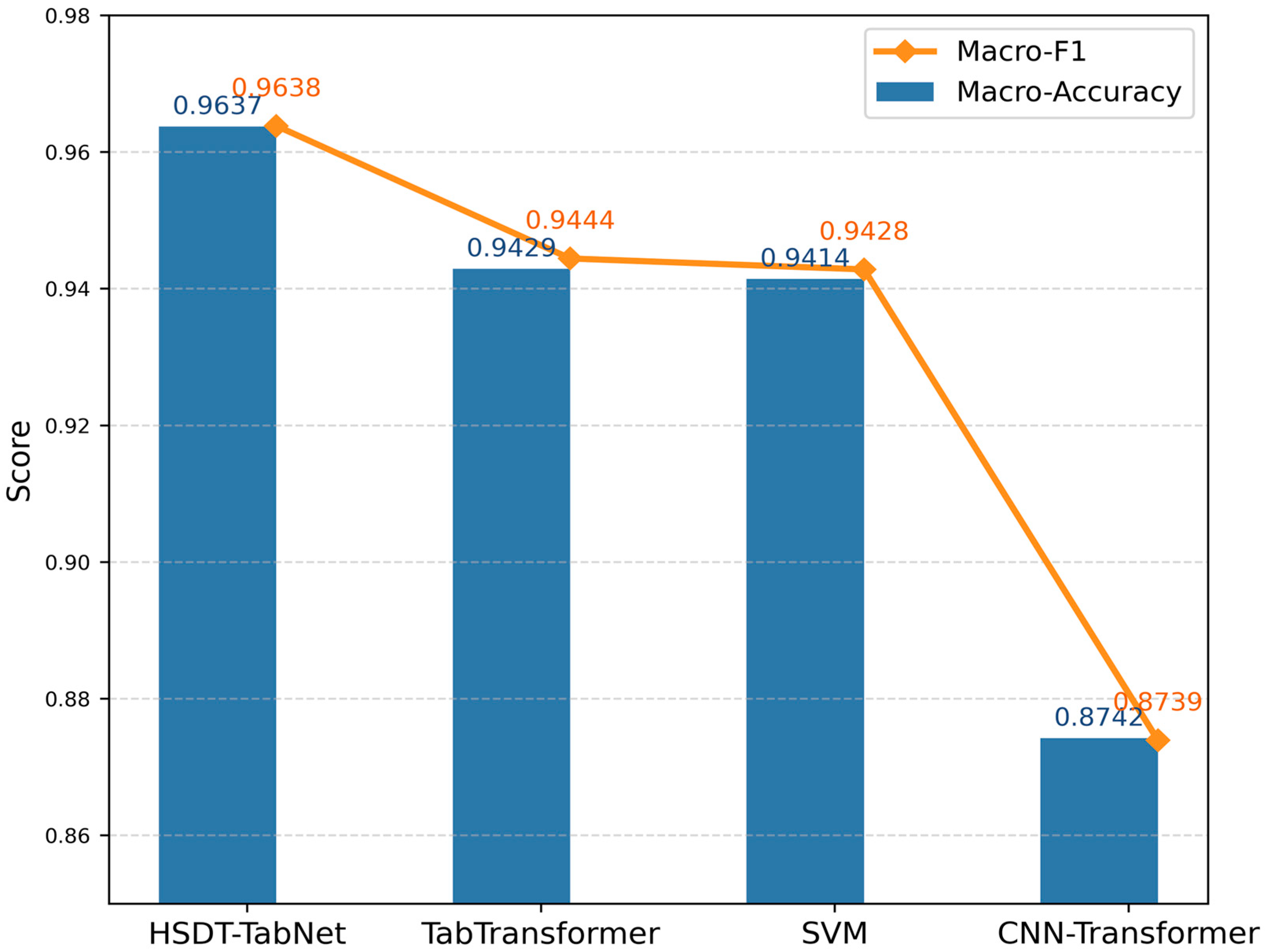
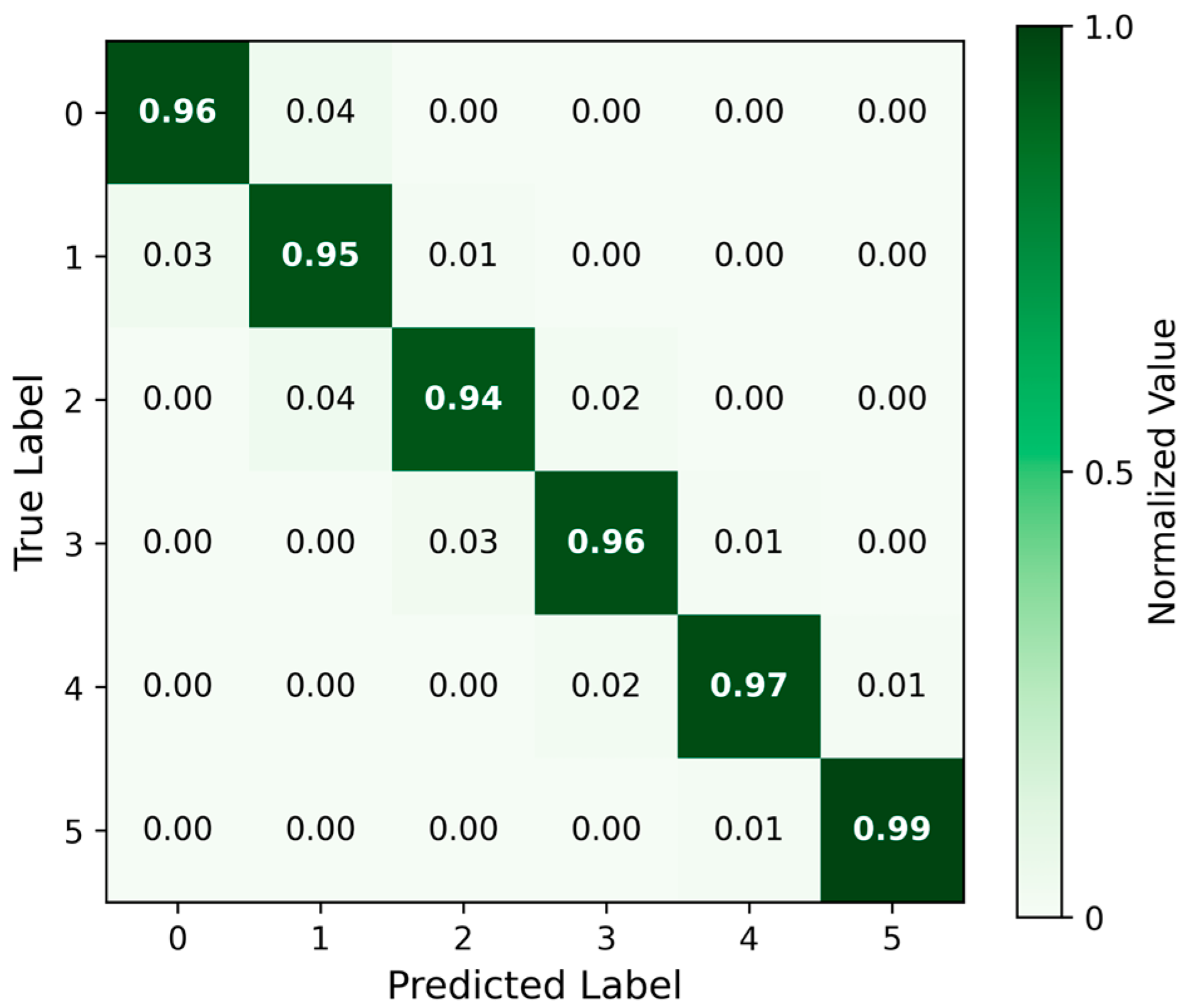
The proposed HSDT-TabNet model demonstrated excellent performance in classifying soybean FLS severity under field conditions, achieving a macro-accuracy of 96.37%, surpassing the TabTransformer model, CNN–transformer model, and conventional machine learning baselines. The significant performance gap compared to CNN–transformer arises from fundamental architectural differences. CNN–transformer leverages the inherent spatial structure of image data, capturing local–global dependencies via convolutional and attention mechanisms. However, hyperspectral reflectance data represented in tabular form lacks the underlying two-dimensional grid structure necessary for these spatial operations to be effective. These results match or surpass those reported in previous controlled-environment studies. For example, Gui et al. [34] developed a CNN–SVM hybrid for early detection of soybean mosaic disease, achieving a test-set accuracy of 94.17% on hyperspectral data collected under laboratory conditions. Feng et al. [8] employed a deformable and dilated convolutional neural network, DC²Net, to detect Asian soybean rust in laboratory conditions, attaining an accuracy of 96.73%. Our dual-path architecture captured the hyperspectral disease signatures as effectively as these specialized models, validating that integrating local and global features is an effective strategy.

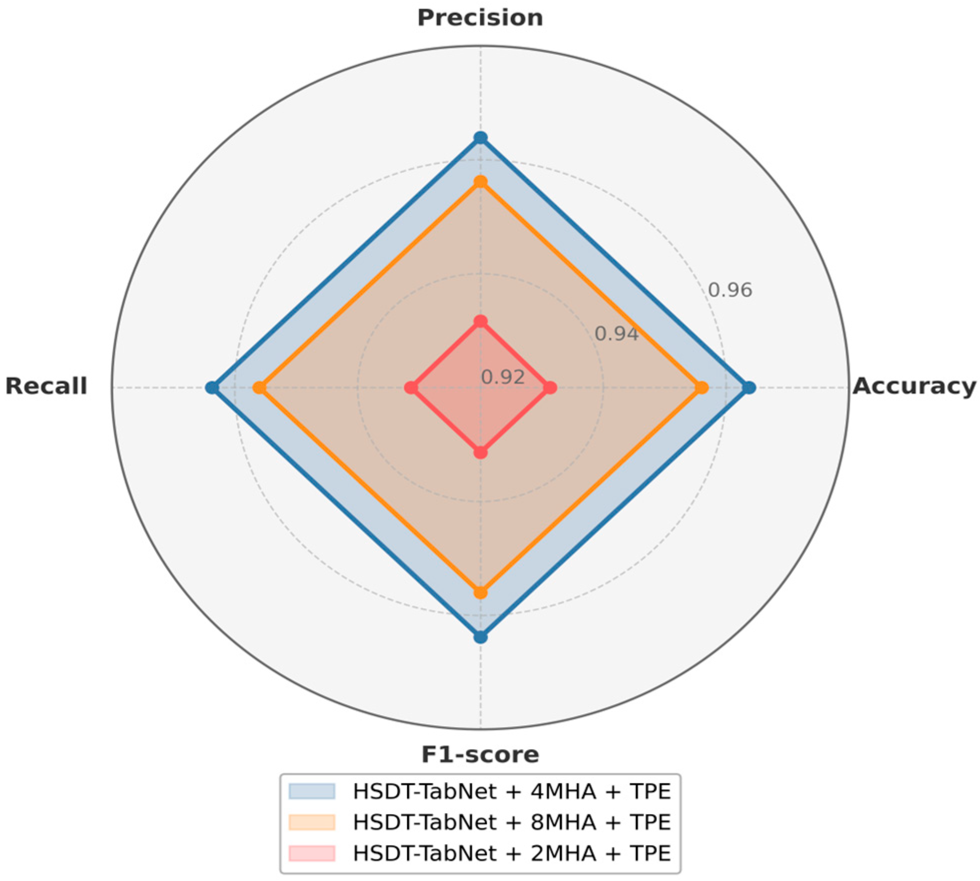
By introducing dual parallel paths, the model leverages the TabNet path to extract sparse local discriminative features, while the HSDT path captures global nonlinear interactions. This synergy increased accuracy by 1.93% over the original TabNet and by 2.39% over standalone HSDT. Hyperspectral tabular data presents unique challenges that make it distinct from typical datasets: it is high-dimensional, often comprising hundreds of spectral bands, which introduces the curse of dimensionality; it typically has small sample sizes due to the high cost and complexity of data collection in field conditions; and it exhibits strong inter-band correlations, leading to redundancy and multicollinearity that can confound traditional models. These characteristics often cause conventional approaches, such as SVM or random forests, to struggle with overfitting or fail to capture the complex nonlinear relationships inherent in the data. The HSDT-TabNet model is specifically tailored to address these issues. The TabNet path employs sparse feature selection to focus on the most relevant spectral bands, effectively reducing the impact of irrelevant or redundant features, while the HSDT path models global interactions across all bands, preserving the overall spectral signature critical for disease detection. Furthermore, the multi-head attention mechanism enhances the model’s ability to focus on different parts of the spectrum simultaneously, capturing subtle and complex patterns that distinguish disease states, particularly valuable when sample sizes are limited. Moreover, we observed that four attention heads (4MHA) outperform configurations with two or eight heads, indicating that while sufficient multi-view projections capture complex spectral–spatial patterns, excessive heads incur diminishing returns and higher variance, consistent with Liang et al. [35], who showed that although multi-head attention enhances expressiveness, too many heads dramatically increase parameter count and computational cost, risking overfitting and instability. In addition, Guo et al. [36] adopted a similar dual-path CNN–transformer architecture and achieved over 97% accuracy on crop classification tasks across multiple UAV-based hyperspectral datasets, further corroborating the merits of hybrid designs. Finally, by employing TPE hyperparameter optimization, we automated the search for critical parameters, improving both convergence speed and generalization ability—thereby validating the effectiveness of this approach.

In severity grading, level 0 (healthy) and levels 4–5 (severe) were easily separable, aligning with the gradual progression of disease [37]. However, soybean FLS exhibits continuity in its levels, with minimal differences in lesion area and severity between adjacent levels, causing blurred boundaries for intermediate levels (1–3) and leading to potential model confusion. Similar observations have been reported in other disease studies [38,39,40], where intermediate stages pose greater classification difficulty under gradual disease progression. To address this, we analyzed misclassifications within the intermediate levels and plan to explore improved optimization strategies to enhance performance in future work.

In summary, HSDT-TabNet was specifically designed for high-dimensional, small-sample, and strong inter-band correlation datasets by integrating dual-path feature extraction, multi-head attention mechanism, and TPE hyperparameter optimization. This approach effectively overcomes the limitations of traditional models in separating local and global features, achieving outstanding performance in hyperspectral crop disease grading tasks and proving particularly suitable for complex agricultural scenarios. The performance gains over traditional baselines, consistent with recent advanced studies, underscore the scientific value of our model. By concurrently modeling local and global feature relations and optimizing hyperparameters, the model markedly enhances detection accuracy and robustness. These findings represent an advancement in UAV-based crop disease monitoring, showcasing the innovation and potential impact of hybrid deep learning models in agriculture.

5. Conclusions

To address the practical needs of soybean FLS severity detection under field conditions, this study proposed an end-to-end HSDT-TabNet model with dual-path feature extraction. The model employs TabNet and HSDT paths to capture local and global features, integrates them via a multi-head attention mechanism, and applies TPE hyperparameter optimization. This enables effective modeling of high-dimensional and small-sample hyperspectral data. On the UAV-acquired soybean FLS dataset, the model achieved a macro-accuracy of 96.37% in five-fold cross-validation, significantly outperforming the baselines represented by TabTransformer and SVM. Future work will focus on optimizing the model to further improve classification performance for intermediate levels and on evaluating the framework’s ability to generalize across a wide range of environmental conditions and multiple soybean cultivars.

The achieved results meet the practical needs of soybean disease monitoring and control, providing a new approach for field-scale severity grading of soybean diseases.

References

1. Dilawari, R.; Kaur, N.; Priyadarshi, N.; Prakash, I.; Patra, A.; Mehta, S.; Singh, B.; Jain, P.; Islam, M.A. Soybean: A Key Player for Global Food Security. In Soybean Improvement: Physiological, Molecular and Genetic Perspectives; Wani, S.H., Sofi, N.u.R., Bhat, M.A., Lin, F., Eds.; Springer International Publishing: Cham, Switzerland, 2022; pp. 1–46. ISBN 978-3-031-12232-3. [Google Scholar]
2. Zhu, W.; Li, J.; Xie, T. Impact of Climate Change on Soybean Production: Research Progress and Response Strategies. Adv. Resour. Res. 2024, 4, 474–496. [Google Scholar] [CrossRef]
3. Butler, S.; Kelly, H.; Mueller, T.; Kruger, G.; Cochran, A.; Raper, T. Influence of Droplet Size and Azoxystrobin Insensitivity on Frogeye Leaf Spot Management in Soybean. Crop Prot. 2018, 112, 149–158. [Google Scholar] [CrossRef]
4. Martinelli, F.; Scalenghe, R.; Davino, S.; Panno, S.; Scuderi, G.; Ruisi, P.; Villa, P.; Stroppiana, D.; Boschetti, M.; Goulart, L.R.; et al. Advanced Methods of Plant Disease Detection. A Review. Agron. Sustain. Dev. 2015, 35, 1–25. [Google Scholar] [CrossRef]
5. Javidan, S.M.; Banakar, A.; Vakilian, K.A.; Ampatzidis, Y.; Rahnama, K. Early Detection and Spectral Signature Identification of Tomato Fungal Diseases (Alternaria Alternata, Alternaria Solani, Botrytis Cinerea, and Fusarium Oxysporum) by RGB and Hyperspectral Image Analysis and Machine Learning. Heliyon 2024, 10, e38017. [Google Scholar] [CrossRef]
6. Alves, K.S.; Guimarães, M.; Ascari, J.P.; Queiroz, M.F.; Alfenas, R.F.; Mizubuti, E.S.G.; Del Ponte, E.M. RGB-Based Phenotyping of Foliar Disease Severity under Controlled Conditions. Trop. Plant Pathol. 2022, 47, 105–117. [Google Scholar] [CrossRef]
7. Zhang, B.; Ou, Y.; Yu, S.; Liu, Y.; Liu, Y.; Qiu, W. Gray Mold and Anthracnose Disease Detection on Strawberry Leaves Using Hyperspectral Imaging. Plant Methods 2023, 19, 148. [Google Scholar] [CrossRef] [PubMed]
8. Feng, J.; Zhang, S.; Zhai, Z.; Yu, H.; Xu, H. DC2Net: An Asian Soybean Rust Detection Model Based on Hyperspectral Imaging and Deep Learning. Plant Phenomics 2014, 6, 0163. [Google Scholar] [CrossRef] [PubMed]
9. Amarasingam, N.; Gonzalez, F.; Salgadoe, A.S.A.; Sandino, J.; Powell, K. Detection of White Leaf Disease in Sugarcane Crops Using UAV-Derived RGB Imagery with Existing Deep Learning Models. Remote Sens. 2022, 14, 6137. [Google Scholar] [CrossRef]
10. Deng, J.; Zhou, H.; Lv, X.; Yang, L.; Shang, J.; Sun, Q.; Zheng, X.; Zhou, C.; Zhao, B.; Wu, J.; et al. Applying Convolutional Neural Networks for Detecting Wheat Stripe Rust Transmission Centers under Complex Field Conditions Using RGB-Based High Spatial Resolution Images from UAVs. Comput. Electron. Agric. 2022, 200, 107211. [Google Scholar] [CrossRef]
11. Jiang, R.; Wang, P.; Xu, Y.; Zhou, Z.; Luo, X.; Lan, Y.; Zhao, G.; Sanchez-Azofeifa, A.; Laakso, K. Assessing the Operation Parameters of a Low-altitude UAV for the Collection of NDVI Values Over a Paddy Rice Field. Remote Sens. 2020, 12, 1850. Available online: https://www.mdpi.com/2072-4292/12/11/1850 (accessed on 9 May 2025). [CrossRef]
12. Santrač, N.; Benka, P.; Batilović, M.; Zemunac, R.; Antić, S.; Stajić, M.; Antonić, N. Accuracy Analysis of UAV Photogrammetry Using RGB and Multispectral Sensors|EBSCOhost. Available online: https://openurl.ebsco.com/contentitem/doi:10.15292%2Fgeodetski-vestnik.2023.04.459-472?sid=ebsco:plink:crawler&id=ebsco:doi:10.15292%2Fgeodetski-vestnik.2023.04.459-472 (accessed on 9 May 2025).
13. Castelão Tetila, E.; Brandoli Machado, B.; Belete, N.A.; Guimarães, D.A.; Pistori, H. Identification of Soybean Foliar Diseases Using Unmanned Aerial Vehicle Images. IEEE Geosci. Remote Sens. Lett. 2017, 14, 2190–2194. [Google Scholar] [CrossRef]
14. Zhang, Y.; Xiao, J.; Yan, K.; Lu, X.; Li, W.; Tian, H.; Wang, L.; Deng, J.; Lan, Y. Advances and Developments in Monitoring and Inversion of the Biochemical Information of Crop Nutrients Based on Hyperspectral Technology. Agronomy 2023, 13, 2163. [Google Scholar] [CrossRef]
15. Colovic, M.; Stellacci, A.M.; Mzid, N.; Di Venosa, M.; Todorovic, M.; Cantore, V.; Albrizio, R. Comparative Performance of Aerial RGB vs. Ground Hyperspectral Indices for Evaluating Water and Nitrogen Status in Sweet Maize. Agronomy 2024, 14, 562. [Google Scholar] [CrossRef]
16. Ali, F.; Razzaq, A.; Tariq, W.; Hameed, A.; Rehman, A.; Razzaq, K.; Sarfraz, S.; Rajput, N.A.; Zaki, H.E.M.; Shahid, M.S.; et al. Spectral Intelligence: AI-Driven Hyperspectral Imaging for Agricultural and Ecosystem Applications. Agronomy 2024, 14, 2260. [Google Scholar] [CrossRef]
17. Abdulridha, J.; Min, A.; Rouse, M.N.; Kianian, S.; Isler, V.; Yang, C. Evaluation of Stem Rust Disease in Wheat Fields by Drone Hyperspectral Imaging. Sensors 2023, 23, 4154. [Google Scholar] [CrossRef] [PubMed]
18. Li, W.; Guo, Y.; Yang, W.; Huang, L.; Zhang, J.; Peng, J.; Lan, Y. Severity Assessment of Cotton Canopy Verticillium Wilt by Machine Learning Based on Feature Selection and Optimization Algorithm Using UAV Hyperspectral Data. Remote Sens. 2024, 16, 4637. [Google Scholar] [CrossRef]
19. Zeng, T.; Wang, Y.; Yang, Y.; Liang, Q.; Fang, J.; Li, Y.; Zhang, H.; Fu, W.; Wang, J.; Zhang, X. Early Detection of Rubber Tree Powdery Mildew Using UAV-Based Hyperspectral Imagery and Deep Learning. Comput. Electron. Agric. 2024, 220, 108909. [Google Scholar] [CrossRef]
20. Meng, W.; Li, X.; Zhang, J.; Pei, T.; Zhang, J. Monitoring of Soybean Bacterial Blight Disease Using Drone-Mounted Multispectral Imaging: A Case Study in Northeast China. Agronomy 2025, 15, 921. [Google Scholar] [CrossRef]
21. Zhang, S.; Huang, H.; Huang, Y.; Cheng, D.; Huang, J. A GA and SVM Classification Model for Pine Wilt Disease Detection Using UAV-Based Hyperspectral Imagery. Appl. Sci. 2022, 12, 6676. [Google Scholar] [CrossRef]
22. Wang, Y.; Xing, M.; Zhang, H.; He, B.; Zhang, Y. Rice False Smut Monitoring Based on Band Selection of UAV Hyperspectral Data. Remote Sens. 2023, 15, 2961. [Google Scholar] [CrossRef]
23. Feng, L.; Wu, B.; He, Y.; Zhang, C. Hyperspectral Imaging Combined With Deep Transfer Learning for Rice Disease Detection. Front. Plant Sci. 2021, 12, 693521. [Google Scholar] [CrossRef] [PubMed]
24. Arik, S.Ö.; Pfister, T. TabNet: Attentive Interpretable Tabular Learning. Proc. AAAI Conf. Artif. Intell. 2021, 35, 6679–6687. [Google Scholar] [CrossRef]
25. Xu, M.; Watanachaturaporn, P.; Varshney, P.K.; Arora, M.K. Decision Tree Regression for Soft Classification of Remote Sensing Data. Remote Sens. Environ. 2005, 97, 322–336. [Google Scholar] [CrossRef]
26. Huang, X.; Khetan, A.; Cvitkovic, M.; Karnin, Z. TabTransformer: Tabular Data Modeling Using Contextual Embeddings. arXiv 2020, arXiv:2012.06678. [Google Scholar]
27. Li, Z.; Chen, G.; Zhang, T. A CNN-Transformer Hybrid Approach for Crop Classification Using Multitemporal Multisensor Images. IEEE J. Sel. Top. Appl. Earth Obs. Remote Sens. 2020, 13, 847–858. Available online: https://ieeexplore.ieee.org/abstract/document/8999620 (accessed on 16 June 2025). [CrossRef]
28. Bhola, A.; Kumar, P. Deep Feature-Support Vector Machine Based Hybrid Model for Multi-Crop Leaf Disease Identification in Corn, Rice, and Wheat. Multimed. Tools Appl. 2025, 84, 4751–4771. [Google Scholar] [CrossRef]
29. Kavitha, T.; Deepika, S.; Nattaraj, K.; Shanthini, P.; Puranaraja, M. Smart System for Crop and Diseases Prediction Using Random Forest and Resnet Architecture. In Proceedings of the 2022 International Conference on Sustainable Computing and Data Communication Systems (ICSCDS), Erode, India, 7–9 April 2022; pp. 1513–1519. [Google Scholar]
30. Hashim, I.C.; Shariff, A.R.M.; Bejo, S.K.; Muharam, F.M.; Ahmad, K. Machine-Learning Approach Using SAR Data for the Classification of Oil Palm Trees That Are Non-Infected and Infected with the Basal Stem Rot Disease. Agronomy 2021, 11, 532. [Google Scholar] [CrossRef]
31. Hayit, T.; Endes, A.; Hayit, F. KNN-Based Approach for the Classification of Fusarium Wilt Disease in Chickpea Based on Color and Texture Features. Eur. J. Plant Pathol. 2024, 168, 665–681. [Google Scholar] [CrossRef]
32. Xing, B.; Wang, D.; Yin, T. The Evaluation of the Grade of Leaf Disease in Apple Trees Based on PCA-Logistic Regression Analysis. Forests 2023, 14, 1290. Available online: https://www.mdpi.com/1999-4907/14/7/1290 (accessed on 16 May 2025). [CrossRef]
33. Heydari, S.; Mahmoud, Q.H. Tiny Machine Learning and On-Device Inference: A Survey of Applications, Challenges, and Future Directions. Sensors 2025, 25, 3191. [Google Scholar] [CrossRef]
34. Gui, J.; Fei, J.; Wu, Z.; Fu, X.; Diakite, A. Grading Method of Soybean Mosaic Disease Based on Hyperspectral Imaging Technology. Inf. Process. Agric. 2021, 8, 380–385. [Google Scholar] [CrossRef]
35. Liang, M.; He, Q.; Yu, X.; Wang, H.; Meng, Z.; Jiao, L. A Dual Multi-Head Contextual Attention Network for Hyperspectral Image Classification. Remote Sens. 2022, 14, 3091. [Google Scholar] [CrossRef]
36. Guo, X.; Feng, Q.; Guo, F. CMTNet: A Hybrid CNN-Transformer Network for UAV-Based Hyperspectral Crop Classification in Precision Agriculture. Sci. Rep. 2025, 15, 12383. [Google Scholar] [CrossRef]
37. Barro, J.P.; Neves, D.L.; Del Ponte, E.M.; Bradley, C.A. Frogeye Leaf Spot Caused by Cercospora Sojina: A Review. Trop. Plant Pathol. 2023, 48, 363–374. [Google Scholar] [CrossRef]
38. Yamamoto, S.; Nomoto, S.; Hashimoto, N.; Maki, M.; Hongo, C.; Shiraiwa, T.; Homma, K. Monitoring Spatial and Time-Series Variations in Red Crown Rot Damage of Soybean in Farmer Fields Based on UAV Remote Sensing. Plant Prod. Sci. 2023, 26, 36–47. [Google Scholar] [CrossRef]
39. Abdulridha, J.; Ampatzidis, Y.; Qureshi, J.; Roberts, P. Identification and Classification of Downy Mildew Severity Stages in Watermelon Utilizing Aerial and Ground Remote Sensing and Machine Learning. Front. Plant Sci. 2022, 13, 791018. [Google Scholar] [CrossRef]
40. Zhang, G.; Xu, T.; Tian, Y. Hyperspectral Imaging-Based Classification of Rice Leaf Blast Severity over Multiple Growth Stages. Plant Methods 2022, 18, 123. [Google Scholar] [CrossRef]
Figure 1. An experimental field layout with 15 soybean plots at varying FLS inoculation levels (A1: control; A2–A5: 1–4 inoculations).
Agronomy 15 01530 g001
Figure 2. Reflectance curves of different disease levels.
Agronomy 15 01530 g002
Figure 3. HSDT-TabNet framework diagram.
Agronomy 15 01530 g003
Figure 4. TabNet path feature extraction framework.
Agronomy 15 01530 g004
Figure 5. A comparison chart of the performance of different attention heads.
Agronomy 15 01530 g005
Figure 6. The performance comparison bar chart of machine learning baseline models.
Agronomy 15 01530 g006
Figure 7. A comparison of macro-accuracy and macro-F1-scores across models.
Agronomy 15 01530 g007
Figure 8. Model cross-validation accuracy box plots for each fold.
Agronomy 15 01530 g008
Figure 9. HSDT-TabNet confusion matrix.
Agronomy 15 01530 g009