Multitemporal Analysis of Land Use Changes and Their Effect on the Landscape of the Jerte Valley (Spain) by Remote Sensing

Abstract

In recent years, the interest of institutions in land use has increased, creating the need to determine the changes in use through spatial-temporal and statistical analysis. This study analyzes the changes over the last 40 years, based on a cartography of landscape units obtained from the study of geo-environmental parameters in the Jerte Valley (Spain) with satellite images, Landsat 5 and 7. Subsequently, through the analysis of spatial patterns and diversity and fragmentation indices, and with the Fragstat software, the landscape was characterized from 1994 to the present. The results show that wooded areas decreased slightly, crops increased in altitude and major environmental disturbances (mainly forest fires) negatively affected the environmental mosaic. Land uses affect the landscape by developing larger tesserae (+5 ha), which are less fragmented (−0.15), but more isolated (0.12). This study demonstrates that landscape metrics can be used to understand changes in spatial pattern, help in decision making to implement appropriate management measures in the conservation of traditional land uses, and allow the maintenance of connecting areas between fragments to avoid the loss of natural corridors to increase landscape quality.

1. Introduction

Landscape can be defined as a spatial configuration of patches of dimensions relevant to the phenomenon under consideration or to the selected organism, which exists only at the moment in which it is perceived by the senses. The landscape can also be considered as a portion of the real world within which we are interested in describing and interpreting processes and patterns; this context can lead to different conclusions, depending on whether we use abiotic and/or biotic factors [1]. These factors make it intrinsically dynamic, both at a temporal [2] and spatial scale [3], since it is conditioned by environmental conditions [4], the ecological processes that take place in it, changes in land use, and anthropic disturbances [5].

Landscapes with marked heterogeneity have a complex structure of habitats, which translates into a high index of diversity [6]. This heterogeneity, as a factor of organization of ecological systems, presents a permanent character of landscapes and determines the generation of differentiated environmental mosaics [7]; which makes their study at a large scale extremely difficult. To the natural dynamics perpetuated by geomorphological [8,9,10], hydrological [11], and biotic [12] processes, to cite some significant examples, we must add human activities, which are currently the main factor in landscape evolution worldwide [13,14,15,16].

Remote sensing imagery is widely used for land cover classification, target identification, and thematic mapping from local to global scales due to its technical advantages such as multiresolution, wide coverage, repeatable observation, and multispectral/hyperspectral–spectral records [17,18]. Several classification methods based on satellite images can be classified as supervised or unsupervised classification methods giving higher priority to supervised classification [19] because of its learning method [20,21].

Each land use class is to an image what a patch is to a landscape mosaic, so with this premise in mind, landscape metrics can be applied to measure the effect of land use changes on landscape shape [22]. Different studies calculated multiple levels of landscape metrics to measure landscape patterns in order to analyze land use, mainly focused on urban land use [23,24,25], and on the classification of satellite images rather than on the analysis of spatial patterns [26]. The research studies where a landscape analysis was performed used metrics based on average patch characteristics [27], ignoring the distribution, size, and changes occurring in the last decades, therefore, this study focuses on diversity indices and indices of the entire landscape.

The implementation of geographic information systems and remote sensing [28] have helped to carry out large-scale landscape studies, and with the support of different spatial pattern analysis programs [29], they have allowed a more precise study of the temporal dynamics of the landscape, which has provided a significant leap in the quality of the studies. For the analysis of spatial patterns, multiple indices have been developed that allow the study of landscape configurations at different temporal moments, evaluating their composition and configuration, the proportion of each class, or the shape of the elements [30].

The objective of this article was to know the effect of changes in land use on the landscape configured as a fluvial-structural valley during the last three decades, comparing the potential landscape with the landscape in 1994, and analyzing the spatial patterns in the subsequent years 2000, 2010, and 2019. Using Landsat 5 and Landsat 8 satellite images, and by analyzing spatial patterns and indices of diversity, dominance, shape, and fragmentation with Fragstat software, four scenarios were characterized and studying their tendency in the configuration of the environmental mosaic allowed us to understand the natural dynamics and the influences of human activities on the landscape.

Landscape metrics and the indices obtained have shown an important role in the analysis of changes in land use, so this study will enable land managers to implement appropriate measures for the maintenance of physical and functional connectivity in an anthropized environment, in order to achieve the objectives, set by the strategies of conservation and improvement of the landscape, for the sake of future sustainability.

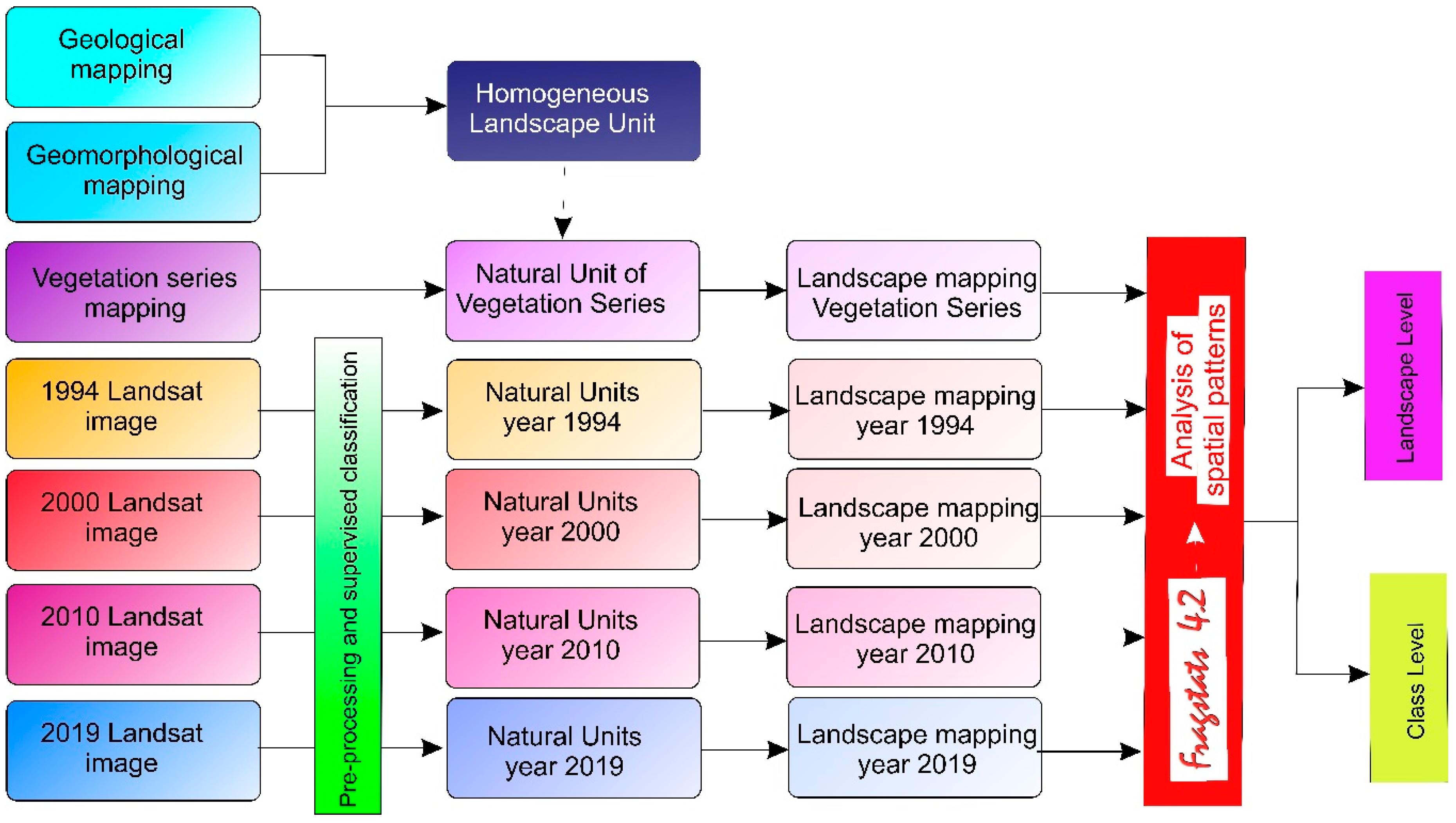
2. Materials and Methods

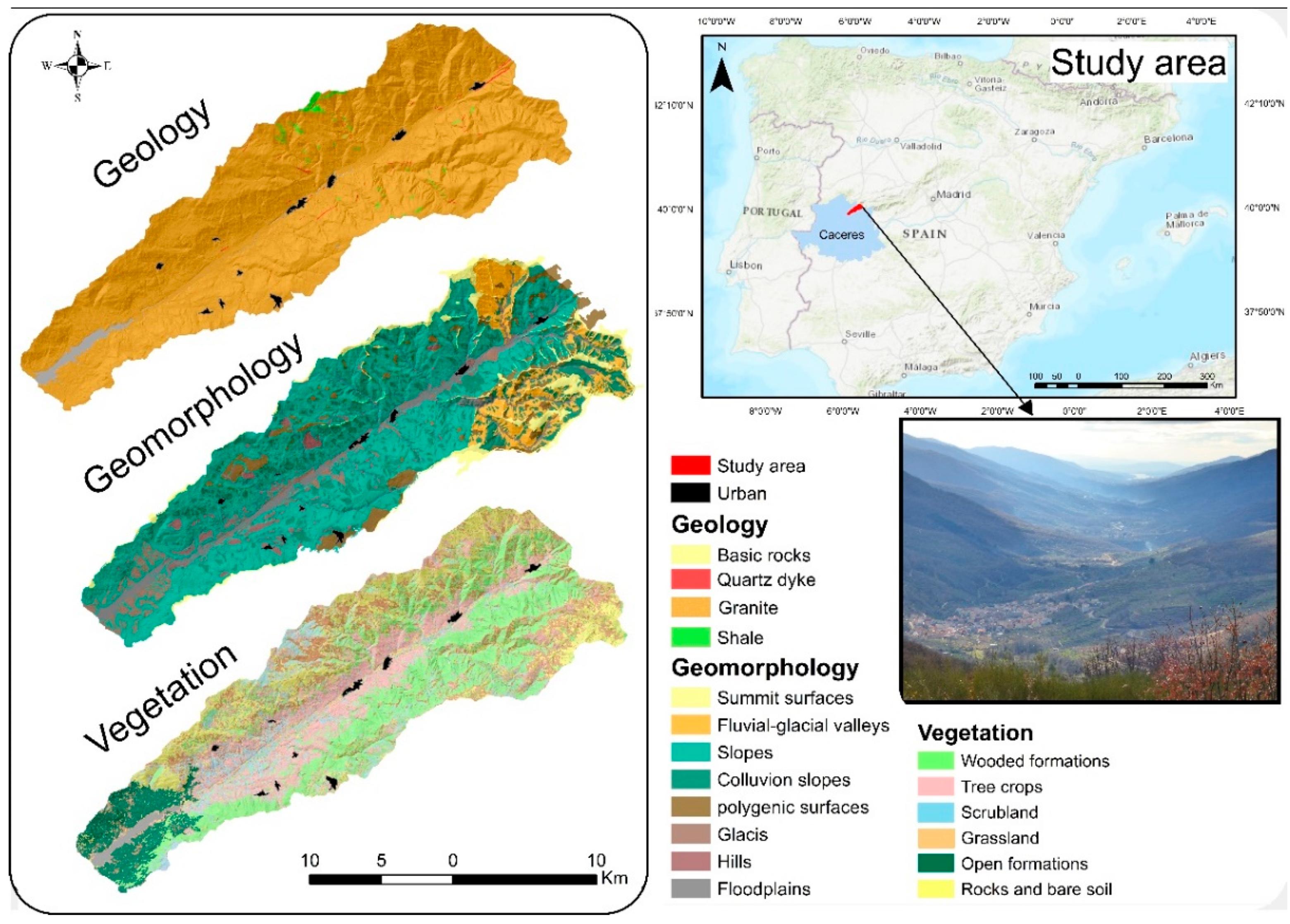
2.1. Study Area

The Jerte valley is located in the north of the province of Cáceres (Spain) (Figure 1). It presents a geomorphological structure of a valley sandwiched between two mountain complexes (Sierra de Béjar, Sierra de Tormantos).

The geology of the study area is mainly formed by granitoids with some quartz outcrops, in the dykes of the Alentejo-Plasencia fault. On the southwestern edge of the study area there are outcrops of metamorphic rocks.

The geomorphological component was obtained based on the mapping of geomorphological units [31], synthesized in a mapping of geomorphological domains. The main geomorphological domains are as follows: summit surfaces and fluvial divides, embedded fluvial-glacial valleys, slopes and colluvial slopes, polygenic surfaces, hills and hillocks, glaciers, and fluvial terraces, alluvial and valley bottoms.

As for the vegetation that develops in the Jerte Valley, it is conditioned by the slopes of the hillsides, the differences in altitude, and the climate. In the areas located to the west, areas of low slope and glacial geomorphology, open formations such as pastures have developed. As one ascends in latitude and altitude there are large extensions of tree crops (cherry trees) very typical of this area. Halfway up the slope, both to the south and north of the river, there are large areas of wooded formations (pine forest, chestnut grove, oak forest, ...). On reaching the timberline, there are different scrublands, and later, ascending in altitude, the summit pastures. Some summits have a steep slope which hinders the development of vegetation while the rock remains on the surface.

2.2. Methods

The methodology followed (Figure 2) for landscape mapping was that described by Martínez-Graña [32], using a supervised classification of Landsat images as vegetation mapping for the years 1994, 2000, 2010, 2019.

With ArcGIS 10.8 software, the mapping of homogeneous units was carried out, from the union between lithology and geomorphological domain mapping. Once the union of these mappings was carried out, 29 homogeneous units were obtained. To simplify these mappings, all units smaller than 2 hectares were filtered out, as they were not representative. The units with similar landscape development behavior, such as quartz slopes and colluviated slopes, basic rock slopes and colluviated slopes, and schist slopes and colluviated slopes, were unified. Finally, the 18 homogeneous units, most representative of the study area, were mapped.

Landsat images were downloaded from the U.S. Geological Survey (https://earthexplorer.usgs.gov/, accessed on 21 July 2021). These images were taken between the months of April, May, or June of the years 1994, 2000, 2010, and 2019. It was decided to use images from Landsat satellites since they were the free satellites with the highest resolution available during the entire study period. The use of images from other satellites, such as Sentinel 2, was considered, but only images from 2015 were available, so we would only have had the latest image to study and with a different resolution, so the surfaces to be compared could have varied. In the end, this option was discarded to homogenize the data as much as possible.

Each image was subjected to radiometric calibration preprocessing, atmospheric corrections, and topographic corrections. Once the images were obtained, training areas were selected after a field reconnaissance and with the help of orthophotos from previous years. Supervised classifications were performed on each image to obtain the land cover. It was decided to carry out the land cover mapping based on supervised classification since high-resolution orthophotos of the study years and field sampling of the last year were available and thus training areas could be delimited with great precision and a highly accurate mapping could be obtained.

Once the study areas were delimited, we proceeded to calculate the spectral signatures of each defined class, in order to extrapolate each pixel value of each class of the training area from the rest of the image. The supervised classification was performed by the maximum likelihood process, this method makes a statistical study (mean and standard deviation) of the pixel values of the training areas and calculates the probability of the values of the external indices to the training areas of belonging to one class or another, while the class with the highest probability is the one assigned to it.

After the supervised classification, a Majority filter was performed, thus filtering the neighboring contiguous cells of the larger size classes and avoiding the salt and pepper effect of supervised classification.

To validate the historical land use mapping, the Kappa index of each supervised classification was calculated. For the mapping to be accepted for further study, the Kappa index had to have been greater than 0.75 [33,34].

Land uses were classified into 10 main classes (water, forest, forest, cherry crops, treeless, scrub, snow, rocky, urban, burned area, clouds) to make the data homogeneous and to be able to analyze their parameters in the landscape as a whole.

The vegetation series mapping used was obtained from the Vegetation Series Map developed by Rivas Martínez in 1981 and revised in 1987 [35]. In the study area there are 5 vegetation series of the 37 existing in Spain. The vegetation series present in the study area have been reclassified (

Table 1. Reclassification of the vegetation series to the legend of the vegetation mapping used for the study.

Vegetation Series	Vegetation Unit
Serie bejarano- gradense silicícola from Festuca indigesta	Grassland
Serie bejarano-gredense occidental and salmantina silicícola from Cytisus purgans	Scrubland
Serie carpetano-ibérico-alcarrena sub-humid silicícola from Q. pirenaica	Wooded formations
Serie luso-extremadurense humid from Q.pyrenaica	Wooded formations
Serie luso- extremadurense silicícola from Q.rotundifolia	Wooded formations
Geoserie riparia mediterráneo	Wooded formations

) in the denomination of the vegetation classes used in the present work in order to make a comparison of potential vegetation and real vegetation.

Then, the corresponding unions of the homogeneous unit mappings with the different vegetation mappings obtained from the vegetation series map and supervised classifications from Landsat images of the years 1994, 2000, 2010, 2020 were carried out, giving rise to the natural unit mappings.

In the mapping of natural units, 53 units were obtained and simplified in the following way:

• Very small units, smaller than 2 hectares, were eliminated.
• Units adjacent and similar to the most representative neighboring units were unified, as long as the extension of the different units was not significant.
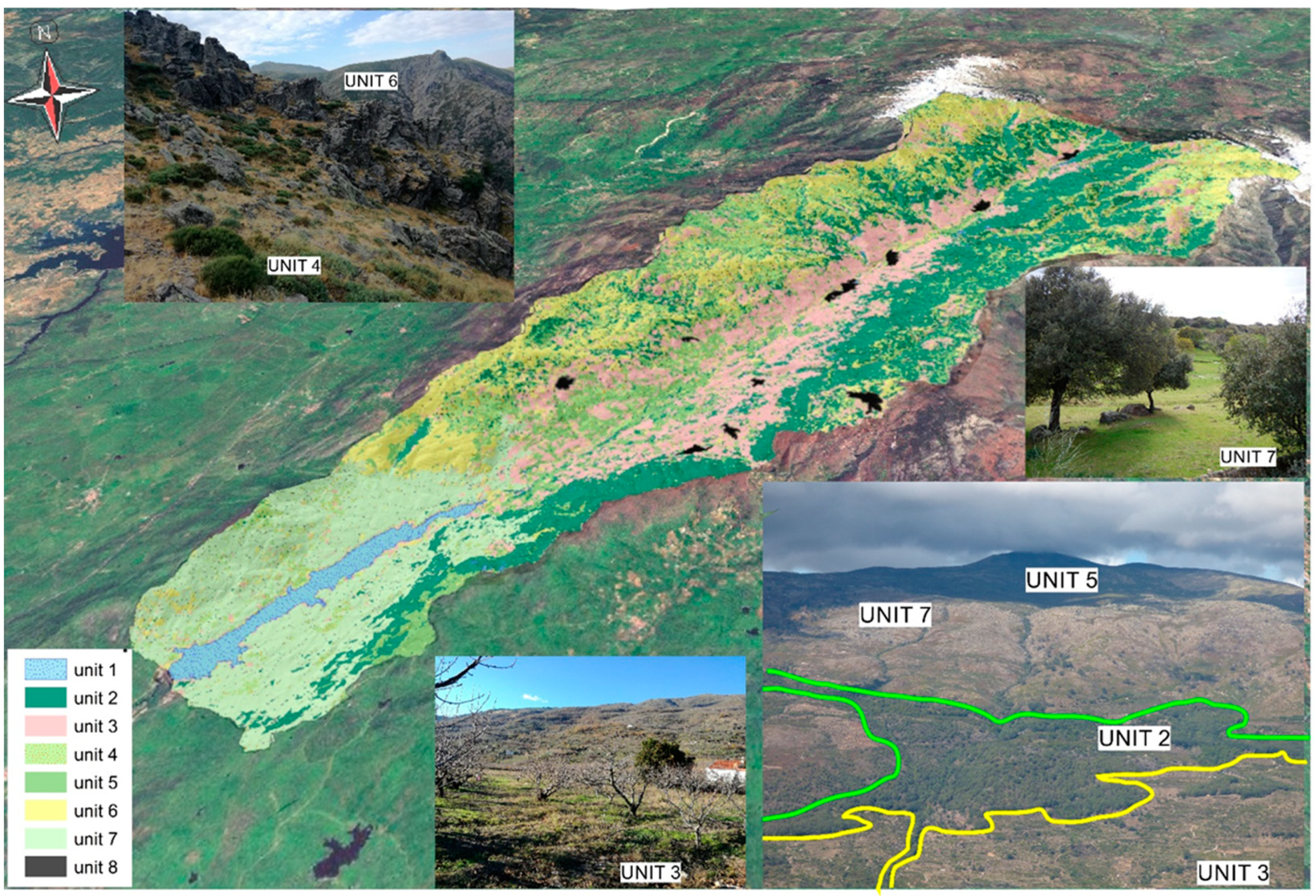
• The field study showed that the simplified landscape units were not representative of the landscape to be studied (Figure 3).
• The result was 8 landscape units (

  Table 2. Ending landscape unit.

  Landscape Units	Characteristics of the Unit
  Unit 8	Urban landscape.
  Unit 7	Glacis and slope in granites with open formations.
  Unit 6	Summits and slopes in rocky outcrop granitoids and bare soil.
  Unit 5	Polygenic surfaces in scrubland granitoids.
  Unit 4	Summits and fluvial-glacial valleys in grassland granite.
  Unit 3	Slope y colluvion slope in granites of tree crops.
  Unit 2	Slopes and colluvial slopes in granites of wooded formations.
  Unit 1	Water landscape

  ):

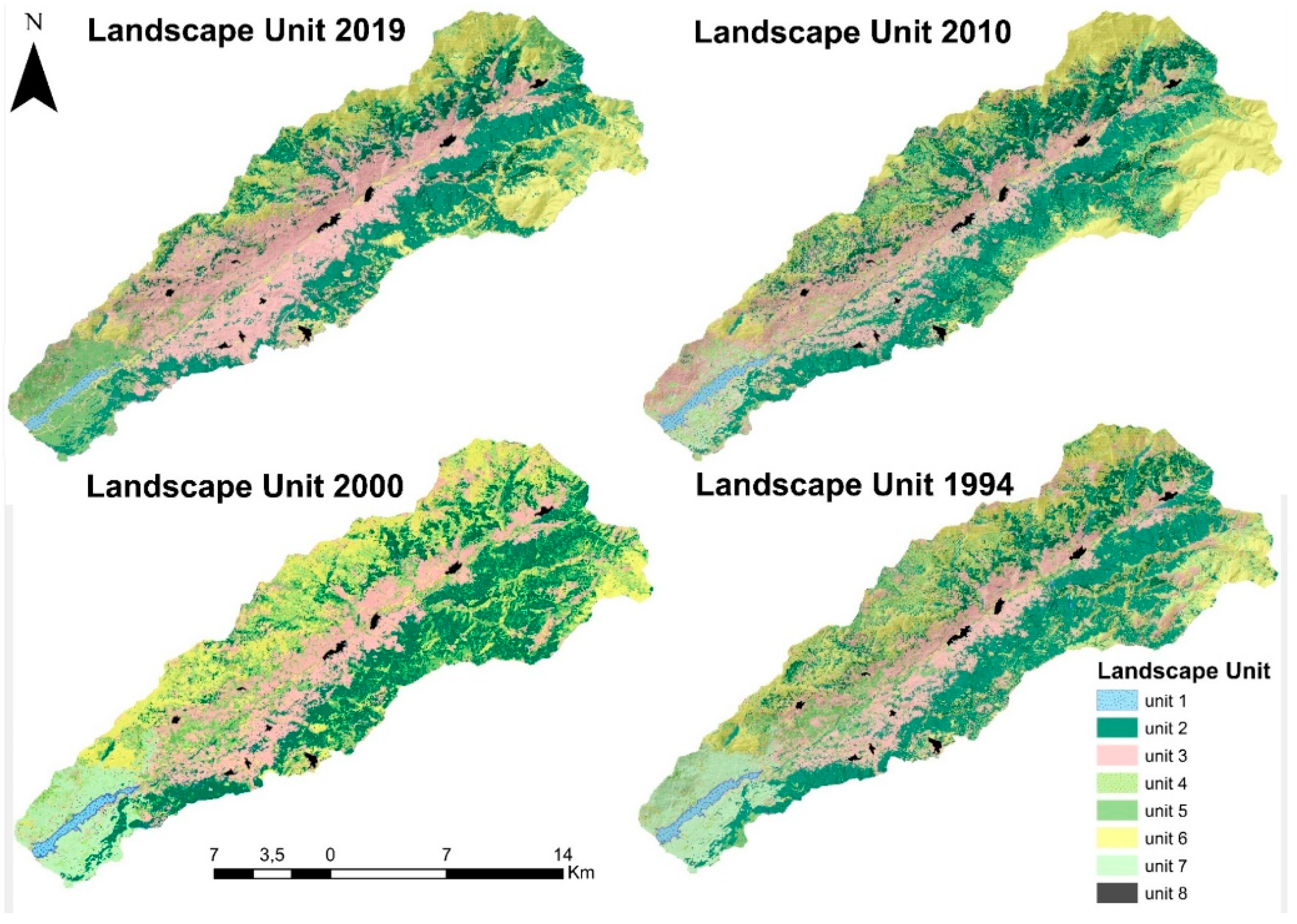
Finally, with the data collected, with the software Fragstat v4.2.1 [36] the analyses of the spatial and ecological patterns of the Jerte Valley were carried out. Fragstat is a software that allows the quantification of landscape patterns, which is a prerequisite for the study of landscape relationships with the processes that degrade it. Fragstat calculates a set of indices and variables that quantitatively describe the level of fragmentation and spatial distribution of land use and land cover.

These analyses were carried out with the help of indices that describe the different classes or patches of the units or allow a description of the landscape as a whole.

The indices used are those described in

Table 3. Index Fragstat.

Index		Observations
Total Area (TA)		TA equals the total area (ha) of the landscape
Number of Patches (NP)		NP is the number of patches of the corresponding patch type.
Mean Patch Area (ÁREA_MN		It is the average of the area of the patches (ha)
Index	Equation		Observations
Radius of Gyration (GYRATE)	${\displaystyle {\displaystyle \sum }_{r=1}^z}{}_Z{}^{Hijr}$ Hijr = distance (m) between cell ijr and the centroid of patch jr, based on cell center-to-cell center distance; Z = number of cells in patch ij.		It is equal to the distance in m, between each pixel of the fragment and its corresponding centroid.
Patch Density (PD)	PD = $\frac{Ni}{A}$ × (10.000) × (100) Ni = number of patches in the landscape of patch type (class) i; A = total landscape area (m2).		Number of fragments in this category for the total area.
Interspersion and Juxtaposition Index (IJI)	$\mathrm{IJI}=\frac{{\sum }_{i=1}^m{\sum }_{k=i+1}^m[\left(\frac{e_{ik}}{E}\times \ln \left(\frac{e_{ik}}{E}\right)\right]}{\ln \left(0.5\left[m\left(m-1\right)\right]\right)}\left(100\right)$ $e_{ik}$ = total length (m) of edge in landscape between patch types i and k; E = total length (m) of edge in landscape, excluding background; m = number of patch types present in the landscape, including the landscape border, if present.		This is the interspersion observed over the maximum probable dispersion according to the number of categories.
Shannon’s Diversity Index (SHDI)	$\mathrm{SHDI}=-\sum _{i=1}^m(P_i\times \ln P_1)$ $P_i$ = proportion of the landscape occupied by patch type (class) i.		Relative abundance of different types of coverage in the landscape.
Shannon’s Evenness Index (SHEI)	$\mathrm{SHEI}=\frac{{\sum }_{i=1}^m\left(P_i\times \ln P_i\right)}{\ln m}$ Pi = proportion of the landscape occupied by patch type I; m = number of patch types present in the landscape, excluding the landscape border if present.		It is the Shannon diversity index divided by the maximum diversity index expected for the classes.
Simpson’s Diversity Index (SIDI)	$\mathrm{SIDI}=1-\sum _{i=l}^m{P}_i^2$ Pi = proportion of the landscape occupied by patch type (class) i.		Probability that two patches belong to the same class.
Patch Cohesión Index (COHESION)	COHESION = $[1-\frac{{\sum }_{j=i}^n{P}_{ij}^{*}}{{\sum }_{j=1}^n{P}_{ij}^{*}\sqrt{a_{ij}^{*}}}]\times {\left[1-\frac{1}{\sqrt{Z}}\right]}^{-1}\times \left(100\right)$ Pij* = perimeter of patch ij in terms of number of cell surfaces; aij* = area of patch ij in terms of number of cells. Z = total number of cells in the landscape.		It measures the physical connectivity of the analysed category.
Landscape Shape Index (LSI)	LSI = $\frac{25E^{*}}{\sqrt{A}}$ E* = total length (m) of edge in landscape; includes the entire landscape boundary and some or all background edge segments; A = total landscape area (m2).		Provides a standardised measure of total edge or edge density to suit the size of the landscape.
Contagion Index (CONTAG)	CONTAG = $[1+\frac{{\sum }_{i=1}^m{\sum }_{k=1}^m[P_{i\times }\frac{g_{ik}}{{\sum }_{k=l}^m{g}_{ik}}]\times [\ln (P_i\times \frac{g_{ik}}{{\sum }_{k=1}^m{g}_{ik}})]}{2\ln \left(m\right)}]\times \left(100\right)$ Pi = proportion of the landscape occupied by patch type; gik = number of adjacencies between pixels of patch types i and k based on the double-count method; m = number of patch types present in the landscape, including the landscape border if present.		It measures the percentage of adjacency between classes, in relation to the maximum possible considering the frequency of these.
Landscape Division Index (DIVISION)	DIVISION = $[1-\sum _{i=1}^m\sum _{j=1}^n{\left(\frac{a_{ij}}{A}\right)}^2]$ aij = area (m2) of patch ij. A = total landscape area (m2).		Probability that two areas of the landscape are not located in the same habitat fragment.
Connectance Index (CONNECT)	CONNECT = $[\frac{{\sum }_{i=1}^m{\sum }_{j=k}^n{c}_{ijk}}{{\sum }_{i=1}^m\left(\frac{n_i\left(n_i-1\right)}{2}\right)}]\left(100\right)$ cijk = joining between patch j and k of the same patch type, based on a user-specified threshold distance; ni = number of patches in the landscape of each patch type (i).		It is the percentage of the total tesserae or of a class connected according to a threshold distance.
Proximity Index (PROX)	PROX = $\sum _{g=1}^n\frac{a_{ijg}}{h_{ijg}^2}$ aijs = area (m2) of patch ijs within specified neighborhood (m) of patch ij; hijs = distance (m) between patch ijs and patch ijs, based on patch edge-to-edge distance, computed from cell center to cell center.		Sum of the areas of tesserae of the same class whose edges are at a specific radius.
Fragmentation (F)	F = $\frac{TA}{NP\times 2\times EN{N}_{MN\times }\left(\frac{PD}{\pi }\right)}$		Spatial disaggregation of patches or habitat types in a given area.

.

3. Results

The supervised rankings performed for the years 1994, 2000, 2010, and 2019 obtained a Kappa index higher than 0.75 (

Table 4. Kappa index and overall accuracy for supervised classification (material complementary).

Year	Parámetros de Imágenes	Kappa Index	Overall Accuracy
1994	LT05_L1TP_202032_19940314_20180217_01_T1	0.92	0.93
2010	LT05_L1TP_202032_20100310_20161016_01_T1	0.76	0.80
2000	LT05_L1TP_202032_20000314_20180312_01_T1	0.88	0.91
2019	LC08_L1TP_202032_20190303_20190309_01_T1	0.86	0.88

), so the mapping was accepted for study:

The changes in land use in the Jerte Valley can be seen in Figure 4. The land use changes obtained in the Jerte Valley can be seen in Figure 3. There is a clear increase in the cultivation of cherry trees, a minimal loss in the extent of forests, with a decrease in scrubland in the years 2000 and 2020 where wildfires were notable.

Based on the maps of landscape units for the study years: 1994, 2000, 2010, and 2019, the data obtained were analyzed (Figure 5). The statistical study began in 1994. Taking as a reference the vegetation series of Rivas Martínez, as potential vegetation, it can be observed that the proportion of land occupied by tree formations is much lower than would be expected (

Table 5. Land cover indices in the Jerte Valley, in the years 1994, 2000, 2010, 2019 and in the vegetation series.

TA	SV		1994		2000		2010		2019
	Total	%	Total	%	Total	%	Total	%	Total	%
Unit 1			433.7	1.10	433	1.10	380	0.98	358	0.92
Unit 2	30,957	82.34	11,103	28.06	9657	24.43	9836	25.29	10,951	28.13
Unit 3			7178	18.14	7486	18.93	7564	19.45	11,271	28.95
Unit 4	76.5	0.20	5257	13.28	5400	13.66	3333	8.57	2176	5.59
Unit 5	4087	10.87	3776	9.54	4913	12.43	3365	8.65	2728	7.01
Unit 6			6368	16.09	6609	16.72	8002	20.57	7187	18.46
Unit 7	2477	6.59	2594	6.55	2334	5.90	2280	5.86	2235	5.74
Unit 8			874	2.21	936	2.47	996	2.56	1386	3.56
Total	37,598		37,598		37,598		37,598		37,598

).

Table 5 also shows how, in 1994, 28% of the surface area of the Jerte Valley was occupied by wooded formations (unit 2), such as oak (Quercus pyrenaica), chestnut (Castanea sativa), and pine (Pinus sylvestris), as opposed to 82% according to the optimum development of the vegetation series. It can also be observed that the presence of grassland areas (unit 3) is higher (13%) due to the traditional cultural uses of the land and its use for grazing, initial stages of recolonization of areas affected by forest fires, deforestation, etc. This stage of landscape development was taken as the initial situation, year 1994, and from there, the changes in the landscape over the last decades were studied.

The development of human activities in the environment has greatly conditioned the landscape in recent decades, occupying the optimal potential areas for the development of tree formations with cherry plantations (28.95%). On the other hand, there is an increase of 57% in the cultivation of cherry trees (unit 2) to the detriment of pasture and scrubland areas, 9% (unit 4 and 5).

The analysis of landscape structure was based on territorial changes in vegetation cover, geomorphology, and land use in recent decades. It was necessary to analyze land cover together with the models and management systems adopted in order to correctly assess the significance of the changes detected.

According to the values obtained in the diversity (SHDI and SIDI) and evenness (SHEI) indices, in the last three decades (Figure 6), heterogeneity and complexity are being lost in the landscape pattern. The number of patches is decreasing, becoming larger, more compact, and with simpler shapes. The grouping of tesserae causes a decrease in ecotones and has direct repercussions on the richness of species present in the environment. This evolution is largely due to the increase in agroforestry practices, forest management, and disturbances such as forest fires.

Once the spatial patterns and metrics of area, density, and landscape aggregation were analyzed (

Table 6. Table of area, density and landscape aggregation metrics obtained by the FRAGSTAT software.

Area, Density and Aggregation Metrics	1994	2000	2010	2019
Total area (TA)	37,598	37,598	37,598	37,598
Number of Patches (NP)	16,023	15,939	9820	8183
Patch Density (PD)	40.48	40.31	25.48	20.69
Radius of Gyration (GYRATE_MN)	47.21	48.90	49.29	57.87
Landscape Shape Index (LSI)	83.32	86.71	50.54	55.25
Mean Patch Area (AREA_MN)	2.47	2.4805	3.92	4.83
Largest Patch Index (LPI)	16.72	10.53	27.25	23.33
Euclidean Nearest-Neighbor Distance Mean (EMM_MN)	141.70	142.01	149.61	166.43
Contagion Index (CONTAG)	30.20	29.10	39.3	40.85
Interspersion and Juxtaposition Index (IJI)	73.55	73.05	70.18	73.00
Connectance Index (CONNECT)	0.36	0.35	0.48	0.48
Landscape Division Index (DIVISION)	0.95	0.97	0.89	0.91
Proximity Index (PROX)	169	124	551	295
Patch Cohesion Index (COHESION)	96.94	96.20	98.38	98.02
Fragmentation Index (F)	0.07	0.07	0.16	0.22

), it could be said that there is an increase in homogeneity at the landscape level in the study area, which corroborates the results obtained in reference to diversity.

The number of patches has almost halved from 16,023 in 1994 to 8183 in 2019. This has caused the patch density to decrease by 50%. Their average area of occupancy has doubled, indicating that we have fewer and larger patches. Likewise, the cohesion index, Landscape Shape Index, and the Interspersion and Juxtaposition Index have increased, which means that the masses maintain a moderately high degree of intermixing despite their tendency to homogenization.

The isolation of the spots increases, with a 74% increase of the proximity index and a 17% increase of the Euclidean Nearest-Neighbor Distance Mean. While the degree of fragmentation decreases by 200% (0.15, remember that it is inverse).

The study of the structure of the landscape at the class level makes it possible to discern the role of each tesserae in the environmental mosaic, assigning to each group a diversifying or homogenizing function in the whole.

The most outstanding results of the study in this area are the increase in the area under cultivation (+7000 ha), dedicated almost exclusively to cherry (

Table 7. Table of area, density, and aggregation metrics of the patches obtained by the FRAGSTAT software. Where: TA: Total area; NP: Number of Patches; PD: Patch Density; AREA_MN: Mean Patch Area; IJI: Interspersion and Juxtaposition Index; Frag: Fragmentation Index.

		Unit 2	Unit 3	Unit 4	Unit 5	Unit 6	Unit 7	Unit 8
1994	TA	11103.25	7178.5	5257	3776	6368.5	874	2594
	NP	2517	2433	3555	3547	2728	825	19
	PD	6.36	6.148	8.983	8.962	6.893	2.085	0.048
	AREA_MN	4.41	2.95	1.47	1.06	2.33	1.05	136.52
	LSI	62.159	63.268	73.399	72.484	62.853	31.445	16.441
	ENN_MN	132.46	139.07	134.83	132.38	138.87	229.17	104.34
	IJI	74.018	78.363	76.914	64.811	72.291	72.84	66.494
	F	0.82	0.54	0.19	0.14	0.38	0.35	4281
2000	TA	9657	7486	5400	4913	6609	713	2334
	NP	2483	2407	3423	3740	2568	965	48
	PD	6.28	6.09	8.66	9.46	6.5	2.44	0.121
	AREA_MN	3.88	3.11	1.57	1.31	2.57	0.73	48.62
	LSI	64.59	63.86	73.26	81.51	62.31	31.97	20.516
	ENN_MN	137.41	138.72	136.27	128.65	142.1	223.7	106.79
	IJI	69.44	80.1	77.24	65.18	74.66	68.72	66.835
	F	0.71	0.58	0.21	0.17	0.44	0.21	589
2010	TA	9836	7564	3333	3365	8002	996	2280
	NP	1523	1600	2620	1489	1811	338	56
	PD	3.95	4.15	6.8	3.86	4.7	0.88	0.54
	AREA_MN	8.76	4.72	1.27	2.26	4.41	1.35	5.11
	LSI	50.53	51.7	58.96	43.5	35.49	19.12	19.13
	ENN_MN	127.05	138.91	147.96	155.86	160.85	217.14	117.58
	IJI	73.75	69.78	74.27	57.78	69.53	74.61	62.09
	F	2.02	1.29	0.2	0.59	0.92	2.43	100
2019	TA	10951	11271	2176	2729	7188	1386	2236
	NP	1143	1216	1707	2064	1334	348	39
	PD	2.89	3.07	4.32	5.22	3.37	0.88	0.10
	AREA_MN	9.58	9.26	1.27	1.32	5.38	1.67	57.32
	LSI	39.08	37.17	46.39	50.75	38.06	20.18	14.65
	ENN_MN	149.84	139.19	178.83	162.20	167.69	269.81	108.49
	IJI	71.53	77.71	78.63	66.25	71.05	66.49	69.90
	F	3.48	3.40	0.26	0.25	1.50	2.63	841

). The tesserae that make up this class increase in number, but maintain the same patterns of isolation, shape, and area. Wooded areas decrease slightly but show changes in their arrangement indicating that the wooded tesserae are larger, less fragmented, but more isolated. On the other hand, units 4 and 5 decrease (3000 ha and 1000 ha respectively) and present very small, isolated, and fragmented tesserae. The open formations (unit 7), due to their singular character, being pasture areas subjected to a strong anthropic influence, require a detailed analysis and study. Large variations in fragmentation are observed, which can be explained by the agrosilvopastoral treatments to which this habitat is subjected.

Valuable assessments can be obtained from the yearly detailed analysis. The year 2010 deserves a special comment since the initial data used for the mapping of landscape units contained parts covered by snow (unit 6). Snow represents an important and common disturbance in vegetation and, in general, in mountain areas. It highlights changes in landscape heterogeneity in annual and sub-annual space. In this particular case, it causes notably high levels in the cohesion and proximity index, and a decrease in the interdispersion and juxtaposition index. In addition, the area occupied by bare soil (snow) increases significantly to the detriment of areas of scrub and grassland, typical of mountain areas where snow accumulates.

Finally, it should be noted that the evolution of urban infrastructures shows a stable, moderate growth and does not represent a problem for the landscape, with diffuse anthropic pressure being practically non-existent, apart from some isolated agricultural and livestock constructions.

4. Discussion

The identification of changes in land use over the last 50 years makes it possible to identify the environmental impact that has occurred in the territory. The decrease in the area of snow, the increase in crop and urban areas, demonstrate an impact generated by anthropogenic activity in the area, mainly by the cherry tree cultivation activity. In other landscape evolution simulation studies, remote sensing techniques were used [33], with classification metrics between 80 and 90% of the images studied for the classification of the extent of tropical forest fragmentation [3] and a supervised classification methodology and landscape indices for landscape fragmentation simulations [37].

The analysis of the areas of occupation of the different types of land use allows a preliminary evaluation of the evolution of the territory. As previously mentioned, the landscape is a dynamic entity in continuous spatial and temporal evolution [38]. The environmental mosaic present in the Jerte Valley is quite heterogeneous and, therefore, the agents that cause these changes are diverse. The most important are: geomorphological agents in the areas of rock and bare soil, where they are the main modelers of the landscape together with the climate; and, in the areas dominated by vegetation, (geobotanical landscape) it is the plants that modify the edaphoclimatic conditions of the area. In addition, we are in a territory with a growing human influence, which determines a much more accelerated time scale of changes due to the disturbances caused by their activities.

Curiously, as a consequence of the change in climatic conditions, the optimal areas for cherry cultivation are no longer the valley bottoms and slopes, but now occupy the higher areas (scrub and pasture). It is a phenomenon marked in other territories with other fruit crops and especially for grapevine [39]. Ultimately it is a consequence of climate change. Presumably, this trend will continue until the lithological and edaphological conditions mean that the land cannot be cultivated, even with the application of the current techniques of farming [40].

Another of the recurrent landscape disturbances in the Jerte Valley and in other areas with a Mediterranean climate are forest fires [41]. At an ecological level, they can be beneficial for the maintenance of the forest structure if they do not occur too frequently, in limited areas, or in areas with a subarid climate. In these cases, they cause simplification of the environmental mosaics [42]. In the study area, forest fires in recent years have mainly affected scrub and grassland areas (see the decrease in the area of occupancy for the year 2020), minimizing their ecological effects, compared to the foreseeable consequences of affecting complex tree formations.

The naturalization of pastures, together with the growth of cherry orchards, has caused the landscape mosaic to change and present more homogeneity and less diversity. It is an unstable and singular situation, since at the same time the natural and cultural landscapes are advancing, giving rise to a common result. This situation can lead to the generation of a cyclical dynamic based on the recurrent occurrence of fires, which is not typical of this territory and can lead to the loss of biological and environmental resources, increased erosion [43], ecological imbalances, etc.

The expansion of cherry trees towards the highlands could be a partial mitigation of the effects described above, enhancing the coexistence of valuable cultural and natural elements. This would favor the maintenance of anthropized areas with lower fire risk and greater economic and ecological potential. Another favorable measure would be the maintenance of extensive livestock farming, both in pasture areas and in mountain pastures, since it plays a fundamental role in the conservation of these habitats, as well as the geobotanical, genetic, and landscape diversity found in them [44].

Dehesa grassland systems have been found to present a high and changing fragmentation of the stippled or mottled type due to the type of management. They are very heterogeneous but harbor a greater diversity than other equivalent potential systems and are therefore a priority for conservation.

5. Conclusions

Previous work has been carried out combining landscape metrics and remote sensing, however, changes in land use have not been studied with this methodology. In the present study, the importance of land use changes in landscape dynamics is highlighted by systematically analyzing landscape evolution using spatial patterns and indices of diversity, dominance, form, and fragmentation. The scenarios analyzed reveal a trend towards homogenization of the territory with loss of diversity and changes in natural dynamics, largely caused by human influence (cherry tree cultivation) and major disturbances created by forest fires.

The research has shown that the analysis of landscape patterns in a multi-temporal study allows both the analysis of changes in past land uses and the promotion of actions for the future conservation of land uses that are positive for the landscape, allowing compliance with conservation strategies, as well as the evaluation of the causes and consequences of large-scale actions or disturbances in the landscape. In addition, the use of geographic information systems, remote sensing, and spatial analysis software allows the evaluation and integration of many geo-environmental parameters that form the landscape, enabling the development of a base cartography of superior detail and quality; and enables the spatio-temporal and statistical analysis of landscape units and their effect on the environment. This methodology can be implemented in different regions with similar characteristics, large areas with a large number of classes, remote regions, difficult to access, etc. For the future, we intend to apply this methodology for shorter time intervals and to see the gradual modification of the landscape for annual periods to observe whether the landscape modifications are gradual or abrupt. It is a fundamental tool for the proper management of land use, land use planning, and environmental conservation. Institutions and territorial managers will be able to adapt the policies and programs of each region to each present and future scenario, adapting this generic methodology to particular situations, thus achieving objective and comparable parameters, extremely useful for decision making.

References

1. Farina, A. Ecología del Paisaje; Universidad de Alicante: San Vicente de Raspeig, Spain, 2011; ISBN 978-84-9717-167-0. [Google Scholar]
2. Hunzkier, M.; Felber, P.; Gehring, K.; Buchecker, M.; Bauer, N.; Kienast, F. Evaluation of landscape change by different social groups: Results of two empirical studies in Switzerland. Mt. Res. Dev. 2008, 28, 140–147. [Google Scholar] [CrossRef] [Green Version]
3. Shi, X.; Feng, G.; Yi, Y.; Zou, Y.; Ge, H.; Su, P. Temporal and Spatial Evolution Characteristics and Ecological Risk Assessment of Land Use Landscape Patterns in Central Zhejiang Urban Agglomeration. Nongye Jixie Xuebao/Trans. Chin. Soc. Agric. Mach. 2020, 51, 242–251. [Google Scholar] [CrossRef]
4. Chhogyel, N.; Kumar, L.; Bajgai, Y. Spatio-temporal landscape changes and the impacts of climate change in mountainous Bhutan: A case of Punatsang Chhu Basin. Remote Sens. Appl. Soc. Environ. 2020, 18, 100307. [Google Scholar] [CrossRef]
5. Cornejo-Denman, L.; Romo-Leon, J.R.; Hartfield, K.; van Leeuwen, W.J.D.; Ponce-Campos, G.E.; Castellanos-Villegas, A. Landscape dynamics in an iconic watershed of Northwestern Mexico: Vegetation condition insights using landsat and planetscope data. Remote Sens. 2020, 12, 2519. [Google Scholar] [CrossRef]
6. Swan, M.; Christie, F.; Steel, E.; Sitters, H.; York, A.; Di Stefano, J. Ground-dwelling mammal diversity responds positively to productivity and habitat heterogeneity in a fire-prone region. Ecosphere 2020, 11, e03248. [Google Scholar] [CrossRef]
7. Li, H.; Reynolds, J.F. On definition and quantification of heterogeneity. Oikos 1995, 73, 280–284. [Google Scholar] [CrossRef]
8. Martínez-Graña, A.M.; Goy, J.L.; Zazo, C.; Silva, P.G.; Santos-Francés, F. Configuration and evolution of the landscape from the geomorphological map in the natural parks Batuecas-Quilamas (central system, SW Salamanca, Spain). Sustainability 2017, 9, 1458. [Google Scholar] [CrossRef] [Green Version]
9. Mariotti, G.; Spivak, A.C.; Luk, S.Y.; Ceccherini, G.; Tyrrell, M.; Gonneea, M.E. Modeling the spatial dynamics of marsh ponds in New England salt marshes. Geomorphology 2020, 365, 107262. [Google Scholar] [CrossRef]
10. Gardner, J. How water, wind, waves and ice shape landscapes and landforms: Historical contributions to geomorphic science. Geomorphology 2020, 366, 106687. [Google Scholar] [CrossRef]
11. Cantonati, M.; Segadelli, S.; Spitale, D.; Gabrieli, J.; Gerecke, R.; Angeli, N.; De Nardo, M.T.; Ogata, K.; Wehr, J.D. Geological and hydrochemical prerequisites of unexpectedly high biodiversity in spring ecosystems at the landscape level. Sci. Total Environ. 2020, 740, 140157. [Google Scholar] [CrossRef]
12. Clément, F.; Ruiz, J.; Rodríguez, M.A.; Blais, D.; Campeau, S. Landscape diversity and forest edge density regulate stream water quality in agricultural catchments. Ecol. Indic. 2017, 72, 627–639. [Google Scholar] [CrossRef]
13. Gao, P.; Kasimu, A.; Zhao, Y.; Lin, B.; Chai, J.; Ruzi, T.; Zhao, H. Evaluation of the temporal and spatial changes of ecological quality in the Hami Oasis based on RSEI. Sustainability 2020, 12, 7716. [Google Scholar] [CrossRef]
14. Rajakumari, S.; Sundari, S.; Meenambikai, M.; Divya, V. Impact analysis of land use dynamics on coastal features of Deshapran block, Purba East Medinipur, West Bengal. J. Coast. Conserv. 2020, 24, 1–10. [Google Scholar] [CrossRef]
15. Rodríguez-Medina, K.; Yañez-Arenas, C.; Peterson, A.T.; Ávila, J.E.; Herrera-Silveira, J. Evaluating the capacity of species distribution modeling to predict the geographic distribution of the mangrove community in Mexico. PLoS ONE 2020, 15, e0237701. [Google Scholar] [CrossRef]
16. Mantero, G.; Morresi, D.; Marzano, R.; Motta, R.; Mladenoff, D.J.; Garbarino, M. The influence of land abandonment on forest disturbance regimes: A global review. Landsc. Ecol. 2020, 35, 2723–2744. [Google Scholar] [CrossRef]
17. Navalgund, R.R.; Jayaraman, V.; Roy, P.S. Remote sensing applications: An overview. Curr. Sci. 2007, 93, 1747–1766. [Google Scholar]
18. Arora, A.; Pandey, M.; Mishra, V.N.; Kumar, R.; Rai, P.K.; Costache, R.; Punia, M.; Di, L. Comparative evaluation of geospatial scenario-based land change simulation models using landscape metrics. Ecol. Indic. 2021, 128, 107810. [Google Scholar] [CrossRef]
19. Du, P.; Xia, J.; Zhang, W.; Tan, K.; Liu, Y.; Liu, S. Multiple Classifier System for Remote Sensing Image Classification: A Review. Sensors 2012, 12, 4764–4792. [Google Scholar] [CrossRef]
20. Abdullah, H.M.; Mahboob, M.G.; Rahman, M.M.; Ahmed, T. Monitoring natural Sal forest cover in Modhupur, Bangladesh using temporal Landsat imagery during 1972–2015. Int. J. Environ. 2015, 5, 1–7. [Google Scholar]
21. Li, C.; Wang, J.; Wang, L.; Hu, L.; Gong, P. Comparison of Classification Algorithms and Training Sample Sizes in Urban Land Classification with Landsat Thematic Mapper Imagery. Remote Sens. 2014, 6, 964–983. [Google Scholar] [CrossRef] [Green Version]
22. Zhang, Y.; Qin, K.; Bi, Q.; Cui, W.; Li, G. Landscape Patterns and Building Functions for Urban Land-Use Classification from Remote Sensing Images at the Block Level: A Case Study of Wuchang District. Remote. Sens. 2020, 12, 1831. [Google Scholar] [CrossRef]
23. Peng, J.; Wang, Y.; Zhang, Y.; Wu, J.; Li, W.; Li, Y. Evaluating the effectiveness of landscape metrics in quantifying spatial patterns. Ecol. Indic. 2010, 10, 217–223. [Google Scholar] [CrossRef]
24. Zheng, X.; Wang, Y.; Gan, M.; Zhang, J.; Teng, L.; Wang, K.; Shen, Z.; Zhang, L.; Campbell, J.; Atzberger, C.; et al. Discrimination of Settlement and Industrial Area Using Landscape Metrics in Rural Region. Remote. Sens. 2016, 8, 845. [Google Scholar] [CrossRef] [Green Version]
25. Aguilera, F.; Valenzuela, L.M.; Botequilha-Leitão, A. Landscape metrics in the analysis of urban land use patterns: A case study in a Spanish metropolitan area. Landsc. Urban Plan. 2011, 99, 226–238. [Google Scholar] [CrossRef]
26. Voltersen, M.; Berger, C.; Hese, S.; Schmullius, C. Object-based land cover mapping and comprehensive feature calculation for an automated derivation of urban structure types at block level. Remote Sens. Environ. 2014, 154, 192–201. [Google Scholar] [CrossRef]
27. Zhang, Y.; Li, Q.; Huang, H.; Wu, W.; Du, X.; Wang, H. The Combined Use of Remote Sensing and Social Sensing Data in Fine-Grained Urban Land Use Mapping: A Case Study in Beijing, China. Remote Sens. 2017, 9, 865. [Google Scholar] [CrossRef] [Green Version]
28. Song, W.; Song, W.; Gu, H.; Li, F. Progress in the remote sensing monitoring of the ecological environment in mining areas. Int. J. Environ. Res. Public Health 2020, 17, 1846. [Google Scholar] [CrossRef] [PubMed] [Green Version]
29. Peng, Y.; Wang, Q. Spatial distribution and influencing factors of settlements in the farming–pastoral ecotone of Inner Mongolia, China. Ecosyst. Health Sustain. 2020, 6, 1771213. [Google Scholar] [CrossRef]
30. McGarigal, K.; Marks, B.J. Fragstats: Spatial pattern analysis program for Quantifying Landscape Structure; USDA Forest Service General Technical Report, PNW-GTR 351; USDA: Washington, DA, USA, 1995. [Google Scholar]
31. Carrasco Gonzalez, R.M. Geomorfología del Valle del Jerte. Las Líneas Maestras del Paisaje; Universidad de Extremadura: Caceres, Spain, 1999. [Google Scholar]
32. Martínez-Graña, A.M.; Silva, P.G.; Goy, J.L.; Elez, J.; Valdés, V.; Zazo, C. Geomorphology applied to landscape analysis for planning and management of natural spaces. Case study: Las Batuecas-S. de Francia and Quilamas natural parks. Sci. Total Environ. 2017, 584–585, 175–188. [Google Scholar] [CrossRef]
33. Anderson, J.R.; Hardy, E.E.; Roach, J.T.; Witmer, R.E. A Land Use and Land Cover Classification System for Use with Remote Sensor Data; US Government Printing Office: Washington, DC, USA, 1976. [Google Scholar] [CrossRef] [Green Version]
34. Olaya, F.V. Sistemas de Información Geográfica, 1st ed.; CreateSpace Independent Publishing Platform: North Charleston, SC, USA, 2020; ISBN 9781716777660. [Google Scholar]
35. Rivas-Martínez, S.; Armaiz, C. Bioclimatología y vegetación en la Península Ibérica. Bull. Soc. Bot. Fr. Actual. Bot. 1984, 131, 110–120. [Google Scholar] [CrossRef] [Green Version]
36. McGarigal, K.; Cushman, S.A.; Ene, E. FRAGSTATS v4: Spatial Pattern Analysis Program for Categorical and Continuous Maps. Computer Software Program Produced by the Authors at the University of Massachusetts, Amherst. 2012. Available online: www.umass.edu/landeco/research/fragstats/fragstats.html (accessed on 15 July 2021).
37. Pyngrope, O.R.; Kumar, M.; Pebam, R.; Singh, S.K.; Kundu, A.; Lal, D. Investigating forest fragmentation through earth observation datasets and metric analysis in the tropical rainforest area. SN Appl. Sci. 2021, 3, 705. [Google Scholar] [CrossRef]
38. Wu, J.-M.; Cai, C.-C.; Sun, H.; Yao, J.-H.; Chen, W.; Gu, J.-S.; Jiang, J.-B. Spatiotemporal evolution and driving force analysis of fractional vegetation coverage over the urban belt along the Yellow River in Ningxia. Arid Zo. Res. 2020, 37, 696–705. [Google Scholar] [CrossRef]
39. Sánchez, Y.; Martínez-Graña, A.M.; Santos-Francés, F.; Yenes, M. Index for the calculation of future wine areas according to climate change application to the protected designation of origin Sierra de Salamanca (Spain). Ecol. Indic. 2019, 107, 105646. [Google Scholar] [CrossRef]
40. Asins Velis, S.; Sánchez Díaz, J. Inclusión de las estrategias de control de la erosión de laderas aterrazadas en las políticas de paisaje. Comun. Congresos. 2011, 565–568. [Google Scholar]
41. Sánchez, Y.; Martínez-Graña, A.; Santos Francés, F.; Mateos Picado, M. Mapping wildfire ignition probability using sentinel 2 and LiDAR (Jerte Valley, Cáceres, Spain). Sensors 2018, 18, 826. [Google Scholar] [CrossRef] [PubMed] [Green Version]
42. Moreno, J.M. Cambio global e incendios forestales: Una visión desde España. In Proceedings of the 4a Conferencia Internacional Sobre Incendios Forestales (CD) DGB/MMA, Sevilla, Spain, 13–17 May 2007. [Google Scholar]
43. Sholagberu, A.T.; Mustafa, M.R.; Yusof, K.W.; Hashim, A.M. Geo-statistical based susceptibility mapping of soil erosion and optimization of its causative factors: A conceptual framework. J. Eng. Sci. Technol. 2017, 12, 2880–2895. [Google Scholar]
44. Vicente Serrano, S.M.; Lasanta Martínez, T.; Cuadrat, J.M. Transformaciones en el paisaje del Pirineo como consecuencia del abandono de las actividades económicas tradicionales. Cons. Super. Investig. Científicas 2000, 155, 111–133. [Google Scholar] [CrossRef] [Green Version]
Figure 1. Study area.
Agronomy 11 01470 g001
Figure 2. General methodology.
Agronomy 11 01470 g002
Figure 3. 3D modeling of landscape units with reconnaissance field images of the most representative landscape units.
Agronomy 11 01470 g003
Figure 4. Evolution of land use in the last 4 decades in the Jerte Valley.
Agronomy 11 01470 g004
Figure 5. Multi-temporal spatial distribution of the natural units in the study area.
Agronomy 11 01470 g005
Figure 6. Diversity indices, the thick lines are the values of the indices in the different years, the thinner lines are the trend of each index. (A) Graph of Simpson’s Diversity Index, (B) Graph of Shannon’s Evenness Index, (C) Graph of Shannon’s Diversity Index.
Agronomy 11 01470 g006