Mapping the Risk of Water Soil Erosion in Larrodrigo (Salamanca, Spain) Using the RUSLE Model and A-DInSAR Technique

Abstract

The quantification of soil loss are studies driven by the importance of soil as a resource and are mainly due to risks of laminar and/or runoff water erosion. These problems directly affect the daily life of the population and serve as predictors of environmental effects. In this work, the quantification and calculation of the sheet water erosion caused mainly by rainfall has been carried out in a study area located in the municipality of Larrodrigo (Salamanca, Spain), based on the simultaneous application of the RUSLE model with GIS techniques. Thematic cartographies have been generated to determine soil loss in Tm/Ha/year and mm/year based on the use of parameters of the physical environment (lithology, rainfall, slopes…) where the erosive risk is quantified and its applicability to the study area by spatio-temporal extrapolation techniques. Simultaneously, the use of the A-DInSAR technique was implemented to calculate average ground deformation velocities in mm/year associated with water erosion. Two sectors with greater vulnerability to water erosion have been detected within the area of interest: one of them called main, which corresponds to the slopes near the Larrodrigo stream, with soil losses showing values of 0.3- > 12 mm/year, and a secondary sector belonging to the tributaries or channels derived from the mainstream with values of 0.3- > 12 mm/year. This type of study makes it possible to manage and organise human support practicesin order to subsequently establish measures that can prevent, mitigate and/or correct those areas with the greatest damage.

1. Introduction

The risk of soil erosion is an issue that has become very important over the years, because soil degradation can cause important environmental impacts and high economic costs, through its effects on the agricultural production, infrastructures and water quality that, in turn, affect the well-being of citizens, potentially threatening their security and representing a serious problem for the sustainable development of the population. On the other hand, organic carbon emissions can be generated from the soil into the atmosphere in the form of CO₂, thus accentuating the effect of global warming [1]. These erosive processes are characterized by being relatively slow and intermittent, although periodic over the years. However, as a consequence of inadequate soil management, erosion from agricultural land can be very intense. Furthermore, soil degradation by erosive agents (water and air) is considered progressive and irreversible since, on the one hand, the volume of soil lost is usually irrecoverable and, on the other, the time required for it to form again, the floor is extremely long [2,3,4].This work will focus on the risks of sheet water erosion or surface rill due to precipitation, which consists of the loss of a more or less uniform layer of soil on a sloping terrain, which mainly affects the released particles by splash. This occurs mainly in situations where the intensity of precipitation exceeds infiltration or when the soil becomes saturated with water, resulting in excess water on the surface. Surface runoff transports the finest particles and causes a decrease in soil productivity (loss of clay, organic matter and nutrients). When the irregularities of the terrain and the greater dolawnstream flow cause the laminar flow to become concentrated, we speak of erosion by furrows, gullies and ravines that represent the three degrees of development of this process. The grooves are centimetric in size and can disappear when carving, the gullies are decametric to metric and generally cannot be removed with ordinary tillage and finally, the gullies are incisions of several meters, even dozens. The result of erosion by gullies and ravines is the dissection of the affected land [2,5]. The area affected by water erosion, as well as its total intensity and magnitude, can be increased by deforestation, forest fires, traditional tillage systems, etc. The absence of plant cover means that the impact of the raindrop not only causes disaggregation, but generally results in the formation of a superficial crust that affects the first millimeters or centimeters of the tillage horizon. This phenomenon is a consequence of the displacement of clay and silt particles that occupy the pores of the soil, causing their occlusion. With this, the infiltration intensity decreases, which favors the initiation of surface runoff [6]. In turn, the same soil, exposed to the action of the same rains, undergoes different erosion intensities depending on whether it is in the upper, middle or lower part of a hilside, and depending on slope (relief effect). Another thing to keep in mind is that the resulting erosion also varies depending on the type of vegetation that protects the soil, the cultivation practices or the use of said vegetation, its disposition with respect to the slope of the slope, and so on. These last two factors, relief and vegetation cover, are what make the erosive action of rain vary on the erodibility of each soil, resulting in different erosion rates in each case, which can be evaluated through the estimation of the effect of each of these factors mentioned.

On the other hand, the application of techniques through Geographic Information Systems (GIS) in environmental studies, allows analysis of the different geospatial databases of the territory to be studied. It is commonly used in areas such as environmental planning and protection, natural resources, natural risk analysis (geomorphological and hydrological modeling, etc.), or the generation of georeferenced thematic cartographies, establishing different analysis methods and models of process simulation [7,8]. The quantification of erosion in the last decades has been carried out by various methods such as USLE, SWAT, MUSLE, PESERA, EUROSEM, etc. which analyze the erosive process considering a static natural environment. For this reason, GIS and remote sensing techniques have made it possible to develop and quantify the parameters that intervene in the erosive process dynamically and with more exact techniques and platforms that have currently been developed (lidar data, satellite images resolution, cartography landuse CORINE-SIOSE, etc). In this article, to detect, monitor and model the erosion risks found, GIS techniques have been used together with the Revised Universal Soil Loss Equation (RUSLE) model, allowing the generation of different thematic cartographies of the territory, for the subsequent analysis of the possible emerging erosion risks (erosive, hydrological, ground movements, geotechnical) and environmental analysis of anthropic actions in the natural environment, at different scales. For the analysis of mass movements or sediment flow there are numerous techniques. The detection process can be carried out: (i) on a local scale, using monitoring systems with sensors such as deformometers, biaxial inclinometers, load cells, flow meters, piezometers, etc. (SIAP MICROS, 2003), which allow alerting in real time, each small landslide or, (ii) at a regional scale through the combined use of the techniques: Geographic Information Systems (GIS) and Advanced Differential Interferometry SAR (A-DInSAR). The Differential Synthetic Aperture Radar Interferometry (DInSAR) technique is based on the calculation of displacement maps of individual events calculating the phase difference (interferogram) of two SAR images obtained over the same acquisition area and orbit, separated in time, allowing the study of the deformation produced by the displacements of the terrain of any area of the planet in a given period of time. Since the beginning of this century, different advanced techniques (such as A-DInSAR) have been developed that allow analysis and studies of slope instabilities and subsidence phenomena through the acquisition and processing of a large number of SAR images, and therefore, of a large number of interferograms [9,10,11,12]. One of the most widely used techniques is the Parallel Small Baseline Subset (P-SBAS), developed and incorporated into the free-to-use platform Grid-Processing On Demand (G-POD) [13]. The SAR images used by this platform come from the ERS-1 and 2 (1991–2011) and Envisat ASAR (2002–2012) satellites. In our case it has been applied to be able to detect, monitor and model differential flows combining A-DinSAR and SIG [14,15].

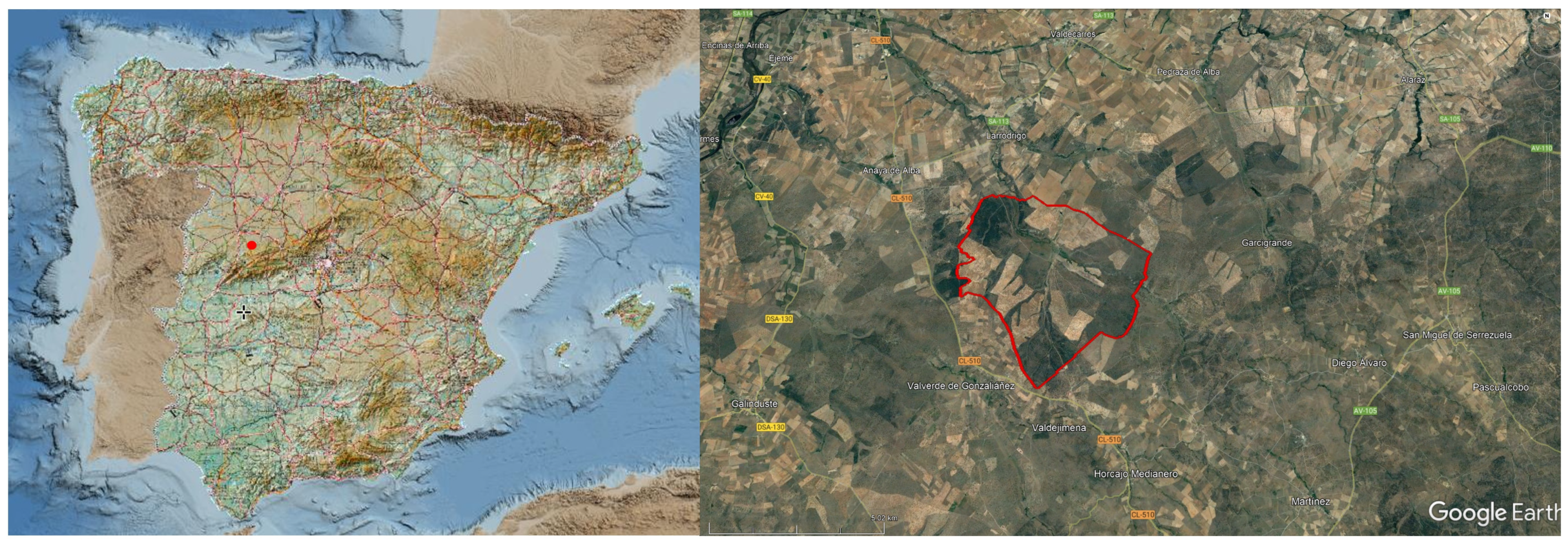
Due to the importance of soil as a fundamental resource for life and the development of anthropic activities, the objective of this work is to quantify the risk of water erosion in an area such as Larrodrigo, with a high capacity for agricultural activity, simultaneously applying the RUSLE method and GIS techniques (ArcGis 10.9, Esri, Madrid, Spain), in order to know the high potential for water erosion risks in the study area. On the other hand, it is intended to detect trends of sediment flows within and in the surroundings of the study area, from the automation of thematic cartographies by means of algorithms obtained from DTMs in order to detect ground movement by applying DinSAR techniques. Finally, for the quantification and calculation of the risk of water erosion, different thematic cartographies generated and mechanized with GIS will be obtained.

2. Materials and Methods

2.1. Study Area

The study area is located in the southeast of the province of Salamanca in Spain and represents an agricultural and livestock exploitation area of almost 2300 hectares in which extensive cattle ranching and organic cereal agriculture coexist. The study area constitutes an area susceptible to water erosion risks, located in an area belonging to the southwestern Atlantic slope of the Iberian Peninsula (Figure 1), with a series of risks of medium and serious magnitude of erosion, especially in agricultural lands, and with tendency to accentuate towards the south. The effects of the physical losses of the soil in the study area are mainly of environmental and economic importance. As mentioned above, this occurs mainly due to surface water erosion of the sheet or gutter type due to its influence on the degradation of natural systems, the loss of land productivity and the alteration of hydrological processes, especially when the anthropically accelerated erosion is considered, which is what causes the great losses of soil. This is mainly caused by the clearing of sloping land, the indiscriminate application of inappropriate agricultural practices, deforestation or large public works. The presence of the Larrodrigo stream and heavy rainfall at certain times of the year, make it the main agents of this type of problem [16].

From a geological point of view, the study area is located on the Central System, close to the northern sub-plateau of the Iberian Peninsula. Formations of tertiary age appear fundamentally which are part of the set of continental facies that fill the Duero Basin. A homogeneity can be appreciated both in the petrography and in the textural context of the differentiated facies, which makes the separation between them very difficult at the outcrop scale, being made from broader criteria based on sedimentological considerations and abundance of structures. There is also the presence of Quaternary age formations superimposed on the Miocene materials. In general, within the study area they can be differentiated from oldest to most modern [17,18] (Figure 2). In the first place, there are deposits corresponding to arches of medium-coarse grain, which include edges of various natures and sizes, which are located scattered in the sands or well grouped, giving more or less continuous levels. Tertiary-age material that is formed mainly by medium-thick quartz grains and, to a lesser extent, by feldspars. The clayey fraction has a reddish tonality and its mica content is abundant. They are located on the southwestern edge of the study area and present hydromorphic processes such as vertically discolorations. The abundance of these discolorations indicates the subaerial exposure of wide areas and the development of vegetation, which requires some time and stability.

On the other hand, arcosic beige sands of Miocene-Pliocene age can be found, which may be affected by a fault and/or be discordant towards the direction SW. They occur throughout the southern half of the study area, and may contain levels of songs that are par-conglomerate with a very abundant matrix, although there may be cases with only one layer of songs or isolated songs. There is very low-angle planar cross-bedding and the- ensemble slopes 5–10° to the direction NNW. In addition, there are large outcrops that correspond to thick white arkotic sands with few clayey intercalations positioned in the northern half of the area of interest. From a lithological point of view, the composition is very similar to that of the San Mamés facies, with a predominance of white-greenish or white microconglomerate sands of low potency and without lateral continuity. They can present some metamorphic rock in the form of an accessory such as slates and more or less altered schists. They contain a monotonous structure, with parallel lamination by alternating sheets of different granulometry, although, locally, very low-angle cross lamination can be observed. They are also from the Tertiary period.

Finally, the quaternary deposits are highlighted. The main generator of this type of formation is the Tormes River and its tributaries such as the Larrodrigo stream, which runs through the study area, due to its large flow. These deposits refer to important terraces located from +18 to +10 m above sea level. These are gravels at the base and predominant sands with edges towards the roof (terraces). There are also fluvial deposits that correspond to the bottoms of valleys and river plains of Holocean age. It extends from north to south and from east to west through the study area following the bed of the Larrodrigo stream and its small tributaries, corresponding mainly to gravels and feldspathic sands. In general, the main load of the riverbed is made up of sand-sized elements, with quartz and feldspar as the majority components, caused by the gentle slope of the riverbeds, making it difficult to remove the thicker edges. Finally, located at the southwestern edge of the study area and superimposed on the tertiary sediments, are the current or sub-current glacis. Its composition is silty-sandy with some sub-rounded edges of variable lithology. The full thickness is not visible, although it sometimes forms a thin layer on the underlying deposits.

The study area constitutes a pilot area in which sustainable agriculture and livestock are developed, supported by the quality and quantity of the existing soil in a fragile ecosystem of Dehesa. Figure 1 shows the changes in land use that have occurred in the sector from 1956 to the present. It is observed how the area occupied by holm oaks has increased considerably, especially in the southwestern sector, while the dehesa areas (term used nationally to describe pastures with holm oaks) have increased slightly. On the contrary, there is a decline in the pasturelands that were cultivated in 1956 and currently host pastures, which is why they are now considered as pastures. Regarding cereal fields and meadows, they have hardly changed.

2.2. Methods

To determine and detect erosion risks that cause soil loss, which are developed in the study area, there are numerous methodology and techniques. There is a first division based on those models that focus on physical processes that take place in erosion (the use of mathematical equations that consider the laws of conservation of mass and energy) and those empirical models that use a series of mathematical algorithms and correlations of erosive factors (although a direct cause-effect relationship with soil losses cannot be established). Due to the complexity of the natural phenomena involved in erosion, there are certain models that have a more probabilistic approach, associating a probability to each erosive event. -The Universal Soil Loss Equation (USLE). Model with greater diffusion and that is used in this project. Proposed by Wischmeier and Smith [19,20] very useful when making decisions about the use and conservation of the soil. It considers six factors and estimates the mean annual soil losses at the level of the agricultural plot or moderately sloping hillside. There is an update and expansion of the model called Revised Universal Soil Loss Equation (RUSLE).

The RUSLE model has been considered the best tool when estimating annual averages of soil losses, in order to inventory and map water erosion in the study area, and is focused on specific restoration plans. environmental and soil conservation. The technique used to develop the RUSLE model is based on the large amount of data collected. In addition, it is a model recognized throughout the world and its application is widespread within the scientific community and in the area of conservation of natural resources. The equation of the model focuses on considering rainfall as the main active agent of this surface erosion, establishing that annual soil losses are directly proportional to the erosivity index of rainfall, related to the kinetic energy of each downpour and its maximum intensity. The same conditions of erosion of the rains can produce different erosions depending on the characteristics and properties of the soil in which they act. With this method it is possible to be able to recognize a series of characteristics of the soil itself that determine its erodibility or vulnerability to erosion, related to its texture, structure, organic matter content and permeability [21].

To calculate the water erosion of the study area, a compilation of cartographic information was previously carried out to later calculate each factor of the RUSLE method. The basic equation of the RUSLE model for estimating average soil losses as a consequence of sheet and trickle water erosion, is A = R × K × L × S × C × P [19,20,22]; where: A are the soil losses per unit area for the period of time considered in Tm/Ha/year. It is obtained by the product of the following factors: R: rain factor (rain erosion index). It is the number of units of the erosion index (E I₃₀) in the period considered, where E is the kinetic energy of a given precipitation and I₃₀ is the maximum intensity in 30 min of it. The erosion index is a measure of the erosive force of a given precipitation given in MJ·mm/Ha·year. K: soil erodibility factor. It is the value of soil losses per units of the pluvial erosion index in t·m²·h/Ha·J·cm, for a determined soil in continuous fallow, with a slope of 9% and a slope length of 22.1 m. L: slope length factor, or the relationship between the loss of soil for a given slope length and the loss for a length of 22.1 m of the same type of soil and vegetation or use. S: slope factor, defined as the relationship between the losses for a given slope and the losses for a slope of 9% of the same type of soil and vegetation or use. C: cover factor and handling. It is the relationship between the losses of soil in a land cultivated under specific conditions or with certain natural vegetation and the corresponding losses of a soil in continuous fallow. P: Factor for soil conservation practices. It is the relationship between the soil losses with cultivation at level, in strips, on terraces, on terraces or with subsurface drainage, and the soil losses corresponding to work on the line of maximum slope [23,24,25]. The equivalence of Tm/Ha/year to mm/year is obtained considering the apparent den-sity, whose value is expressed in gr/cm³. To calculate the thickness 1 Tm/Ha of each soil in mm, the relationship between soil loss (gr/Ha) and apparent density (gr/Ha) is considered. The methodology followed is summarized in Figure 3 and will be explained step by step in the following subsections.

In the Figure 3 with the RUSLE model, a digital terrain model of the area of interest was created from LIDAR data and the application of A-DinSAR techniques was carried out to be able to observe some movement of the terrain.

2.2.1. Compilation of Cartographic Information of the Study Area

Relevant information was collected from the study area that refers to topography, lithology and relief: Orthophotography (Download Center of the National Geographic Institute -IGN-), a set of four raster files that correspond to the most current PNOA orthophotos from part of the province of Salamanca covering part of the geological sheets 1:50,000 of Salamanca and Ávila. LIDAR images (Spatial Data Infrastructure Download Center of Castilla y León, Idecyl), LAZ file package. corresponding to the LIDAR data of sheet 212 of 2010 of Castilla y León covering the study area. Raster maps at a scale of 1:50,000 and in greater detail at 1/25,000 IGN-, which present toponymic information of the study area. Information on pluvio-metric and thermopluviometric meteorological stations (Geo Portal, Ministry of Ecological Transition), with a total of 58 files that show information about the geographical position, altitude, average monthly rainfall and maximum rainfall in 24 h of the stations close to the study area. Reference geographic information (BCN200) such as the regional and national road network, elevations, urban centers, drainage network, etc.

2.2.2. Field work

A field campaign was carried out in order to visualize the erosive state of the areas most affected by water erosion, especially those that are very close to the main channel. Several field campaigns have been carried out and a series of images was captured of the most significant footprints that verify the passage of water erosion in the area of interest. This type of campaign helps to have a preliminary visualization to carry out the analysis and geospatial modeling of the risk of water erosion in order to contrast what is observed in the field with the results obtained from the complete study (Figure 4).

2.2.3. LIDAR Data Application for the Creation of the Digital Terrain Model -DTM-

LIDAR data collects altitude data allowing to define the terrain surface and generate digital elevation models. They are massive point cloud datasets that can be managed, visualized, analyzed, and shared using GIS. In order to work with this information, it is necessary to download LIDAR data clouds, for this there are several sources of information worldwide such as the online LIDAR project that seeks to group this type of data and offer it free of charge. In the case of Spain, there is a spatial data infrastructure (www.idee.es) where data, metadata, services and geographic information produced at the state level are integrated through the internet regional and local. In addition, there are projects such as PNOA-LIDAR which can be purchased from the download center of the National Geographic Institute (IGN) or from the Autonomous Communities’ portals. In this case, when the study area is located in Castilla y León, the LIDAR data will be obtained from the Idecyl. The file package or batch LIDAR_CyL_2015_h10_0529.laz belonging to the study area was chosen. A conversion is needed in the LAZ file format (LIDAR data) in LAS format so that ArcGIS can visualize it, for this, the LASTools tool package is used. The DTM is generated from the LAS files. It is necessary to filter the LIDAR data in such a way that only the terrain height data is kept and not the surface data (which includes, for example, the vegetation height). Such a filter can be done using other LASTools software or directly from the GIS ArcMap as in this case. A DTM is created with the highest possible resolution due to the size of the study area, so the assignment of the values to the cells and the cell size of the raster will be 1 (to create cells with 1mx1m resolution). Finally, the DTM of the study area is obtained, which will be the basis for obtaining different factors from the RUSLE model (Figure 5).

2.2.4. Use of the Free use Platform G-POD for the Application of the A-DInSAR Technique

Access to the free-to-use platform G-POD is done through the web https://gpod.eo.esa.int/ (accessed 20 October 2021), where a user account is created by registering in the system. Within the platform, the A-DInSAR, SBAS-InSAR technique will be used, which is the one of interest in question for the study. Once within the service, the user selects the study area and checks the availability of the SAR images for the area and the dates to be analyzed. (Figure 5A). The objective of this methodology is to be able to develop a SBAS-InSAR technique linked to the G-POD platform, based on the formation of displacement maps of individual events calculating the phase difference (interferogram) of two SAR images obtained on the same acquisition area and orbit, but temporarily separated by acquiring a series of satellite images for subsequent processing in order to obtain information about the average deformation speeds of different points on the ground in the study area.

This technique allows directly the acquisition of satellite images that focuses on obtaining displacements generated in a determined interval of time to visualize the temporal evolution of the displacements of the terrain of the study area, calculating the difference between each displacement in time. The selected images that will later follow the SBAS-InSAR processing follow this procedure: first the choice of the dates of the desired images. The search carried out was ten years from 1 January 2002 to 31 December 2010. But the images that were processed were between March 2003–January 2010. Second, determination of the coordinates of the study area (longitude and latitude) indicating the type of virtual file 4 (VA4) or G-POD. In our case, a VA4 file will be obtained with a RAM label. The track number is a parameter that limits the number of images of interest in the delimited area. When searching for images, the system offers several image packages, using track number 459. The data used will be of the ASAR type because it automatically suppresses possible duplicate images and correctly correlates SAR data that are part of different image packages. the same sequence. This number is chosen based on the availability of the number of images each track contains, the orbital of the satellite and the conditions of the study area. To determine the appropriate track, the platform provides information about all available track numbers of the desired delimited area (http://esar-ds.eo.esa.int/socat/ASA_IM__0P_Scenes) (accessed 20 October 2021).

The images are processed from the SBAS-InSAR database, and for this study 62 SAR images were acquired from the Envisat ASAR satellite, with dates from April 2003 to January 2010. The main characteristics of the images are as follows: Level 0 ASA_IM_OP, track 459 and ascending orbits images (Figure 5B). Subsequently, with the desired image package, the reference point of the displacement measurements generated by the SBAS-InSAR algorithm is established by manually inserting the geographic coordinates of the location or by moving the halo found in the viewer of the platform. To facilitate the process, the largest number of urbanized areas and towns are included to reference the points. Subsequently, the Perform multitemporal analysis that generates time series of displacements through SBAS-InSAR. By selecting this option, the Publish Inter-ferograms check box is available, which allows the user to download the interferogromas generated during the SBAS-InSAR processing chain. Once the type of processing and the Cat Data Over Selected AOI check box have been chosen, the system delimits a square of the area of interest that will be the data that the identified AOI automatically processes (Figure 5B). There is an advanced configuration box in which you can modify the different parameters it contains, to specify the type of images package with greater precision. Normally this type of box is used by specialized people and dedicated to this type of platform G-POD and ABAS-InSAR and not beginner users (Figure 5C). Once the processing has started, the user can view the evolution of the different stages that take place during the A-DInSAR processing: co-registration of the SAR images, formation of the rolled differential interferograms, unrolling of the phase of the interferograms, estimation of the linear velocity, geocoding of velocity points, etc. The processing time of the images is totally dependent on the platform system, so it may vary depending on the availability of the G-POD. For our area, the processing time has been 48 h. A total of 64 interferograms were processed (Figure 5D). The final result is a set of points that shows the displacement speed of a given place within the area of interest in mm/year and the time series of deformation (accumulated deformation over time) of the study area in part ticular. After finishing the process, you can see the evolution of the processing and the time interval that it takes in the workspace, in which you can also see the summary of the process (task ID, Service used, task status, progress, time of creation, presentation time and completion time). The folder with the final result is the most important of the entire process since it is the result of the entire DinSAR methodology showing the average speed of land displacement in the study area mm/year.

The points obtained show a coherence scale of 0–1, with 1 being the maximum possible coherence and 0 the minimum, referring to this concept to the validity of the point as data, that is, to the degree of quality of co-registration between the images. HE. In this way, the algorithm implemented in P-SBAS directly eliminates the points that contain a coherence below 0.7, considering them null values of low validity, keeping all the points that are above that threshold. The points considered valid, contain a very high coherence, so when studying them they are very reliable. To facilitate the processing of the images and to obtain a good coherence of the data, it is necessary to verify that the coordinates entered are always on land and within the selected area. To make the process easier, urbanized areas are usually the most useful for locating reference points, since in them anthropic structures with the presence of planes, corners and straight forms, in general, are easily recognizable. The A-DInSAR information acquired is provided in a kmz file (for viewing in Google Earth) and a document in txt format where the characteristics of the acquired points are presented: point IDs, geographical coordinates in WGS 84, topographic elevation, mean velocity (mm/year), coherence value and deformation time series. This document is exported to a GIS (Figure 5E). Before finalizing the A-DInSAR methodology, all the information about the images processed in the G-POD platform will be collected in a database provided by the European Space Agency (http://esar-ds.eo.esa.int/ socat / ASA_IM__0P_Scenes) (accessed 20 October 2021).

2.2.5. Calculation R Factor or Climatic Aggressiveness/Pluvial Erosivity

Based on the monthly mean rainfall and the maximum rainfall in 24 h, the rainfall erosivity is calculated using the R index. Information was obtained from a total of 28 meteorological stations indicating the name, code or code of the station, its UTM 30N coordinates, its monthly average rainfall values. With all this data, an Excel table is created that is imported into ArcGIS. From the geodatabase, a point layer is created where some projected coordinates ETRS_1989_UTM_Zone_30N are entered. From this spreadsheet a point layer is obtained in vector format that reflects the geographical position of each one of the meteorological stations as its average monthly rainfall and maximum rainfall in 24 h. (Figure 6). With the vector file of the stations, the precipitation erosivity factor (R) is calculated according to the modified Fournier index (MFI). To obtain the aggressiveness of the rain, you must have the precipitations in raster format for each month. To do this, an interpolation is carried out, using the inverse of distance-IDW method. Through this method, the value of each cell of the raster is calculated as the weighted average of the values of the environment as a function of the inverse of the distance, so it is interpreted that the closest points will contain greater relevance. Interpolation is performed for each month (from January to December) with a cell size of 1 × 1 pixel to have the highest possible resolution. With the raster cartography of each month, the rain erosivity index is calculated from the Equation (1) and for the calculation of the IFM we use the Equation (2), where Pi is the precipitation of each month in mm and Pt the mean annual precipitation in mm. Each of the previously generated rasters correspond to each of the 12 values of Pi, so that from them the final raster that represents the value of the mean annual precipitation (Pt) can be obtained, being the sum of all the monthly values of precipitation. Applying map algebra, we do the summation of the monthly layers obtaining the map called Pt. Finally, with all the calculated values of the Equation (1) is applied with the raster calculator and the final result is a raster that shows the different values of the R index in the study area and its surroundings. As a final action, it is necessary to cut the relevant information that only refers to the study area (Figure 6A):

$$R=2.56\times IF{M}^{1.065}$$

(1)

$$IFM={\displaystyle \sum }_{i=1}^{12}\frac{P{i}^{\left(2\right)}}{Pt}$$

(2)

2.2.6. Calculation of the K Factor or Resistance to Soil Erosivity

The K factor is a direct indicator of the erodibility or erodibility of the soil, specifically it reflects the lithological and edaphic vulnerability to erosion, calculated from the physical properties of the soil and the rocky substrate [26,27,28,29]. Linking the lithology of the study area with the K factor is key, since each type of existing lithology will have a specific value of the K factor, varying the vulnerability to erosion. In the calculation of the K factor, the lithological analysis is carried out according to the lithological resistance in those areas where the rock outcrops and the edaphological analysis by means of experimental plot stations and with analytical samplings.

Twelve stations of 20 m² that overlap with the geological cartography have been considered to determine their lithology. The analysis and improvement of the value of the K factor is carried out next with the edaphic analytical study located on each rock substrate [30]. For this we use the nomogram of Wischmeier and Smith and the Wischmeier regression equation (Equation (3)) [22] from the experimental data obtained with simulated rains, where: M = texture (100% clay) × (% silt + very fine sand), a = % organic matter, b = type of structure, c = permeability class. Finally, the K factor is obtained according to each soil, which reflects the difference in resistance to erodibility and ero River hydrographic basi the edaphic vulnerability to erosion of the desired area as a function of the soil. (Figure 6B). A field sampling has been carried out analyzing the upper 20 cm of the soil to analyze the percentage of organized matter and thickness of the A horizon:

100 … K = [10 − 4 … 2.71 … M^1.14 … (12 − a)] + 4.2 … (b − 2) + 3.2 … (c − 3)]

(3)

2.2.7. Calculation of the LS Factor

This type of factor encompasses two topographic parameters that refer to the length of the slope (L) and its slope (S). To calculate its value, the Equation (4) [31]:

LS = 〖Flow accumulation × (cell size/22.13)〗^0.4 × 〖(SineSlope/0.0896)〗^1.3

(4)

Where the flow accumulation is the number of cells that contribute to the flow in each given cell, the cell size is the length of the cell size used throughout the methodology and the SineSlope is the sine of the slopes in radians. First, the slopes (S) are calculated in degrees from the digital terrain model and the values are transformed into radians by multiplying each pixel of the raster map by π/180 applying map algebra. Subsequently, we continue with the calculation of the slope length (L) from obtaining the flow accumulation raster and the flow direction. The accumulation of flow is then multiplied by the cell size, which represents the length of the water path. A maximum slope length of 250 m is established in a standardized way, which is equivalent to 250 cells or pixels and the special resolution of the raster is 1 m × 1 m. Taking this into account, we elaborate a flow accumulation map whose maximum value is 250, this means that the cells in the tracker or accumulation map whose value is less than 250 must retain their original value, but instead, those that present higher cell values, they must all take the value of 250 (maximum value set). Two new layers of accumulation of the flow will be created from the original calculated, using reclassification algorithms, where: Layer A: If the accumulation flow is ≤ 250, it takes value 1; if the accumulation flow > 250 takes value 0; y Layer B: If the accumulation flow is ≤ 250, it takes value 0; if the accumulation flow > 250 takes value 250. Next, the accumulation of the original flow will be multiplied by Layer A, obtaining a file that preserves the original values except for those cells where the original value was greater than 250, which now It will be 0. Once this is done, Layer B is added to the new calculated layer so that those cells that have a value of 0 will take the value 250, which is the maximum that we wanted to set. The final mapping of the LS factor is obtained by applying the Equation (4) using raster calculator (Figure 6C).

2.2.8. Calculation of C Factor or Vegetation Cover

Factor C or Vegetation Cover considers the management of plant and crop masses; Therefore, based on the land uses obtained from the most current PNOA orthophoto and the forest map of the area, we can identify the type of vegetation and its density (Figure 6D). This factor analyzes the influence of the type of land use according to its plant species cover, the alternation of crops influencing the degree of erosive susceptibility of the land, which will influence its productivity. To obtain Factor C we use the reference tableand the values established by the United States Soil Conservation Service [3,21,32,33,34,35,36], for arboreal, shrub and mixed wooded formations, analyzing the percentage of tree and shrub cover; type of herbaceous cover and thickness of plant offal and extension. Regarding the herbaceous formations, the Wischmeier Table has been considered.

2.2.9. Obtaining the Potential and Current Erosion Risk Cartographies

Once we have all the calculated factors involved in the RUSLE model, the risk of potential erosion can be established, conditioned by the combined effect of the factors rain, runoff, soil and slopes. This cartography is obtained from the product of the factors R, K and LS generating a potential erosion map. To determine the degree of existing soil loss, the “present moment” is considered by analyzing the generating and protective factors of the soil; as well as their spatial distribution (types of cultivation and autochthonous plant masses, conservation practices). Basically, it is obtained from the product between the potential erosion calculated previously with the C factor of the RUSLE model, since the vegetation plays a fundamental role when it comes to the development of the erosion that may be generated [37,38,39]. Conservation practices have not been considered (RUSLE P factor = 1) given their lack of consistency and also the interest in calculating natural erosion without human support practices (both positive and negative) to establish the best land uses favoring edaphic recovery. In the erosion risk cartographies can be seen that soil losses per unit area increase with the increasing length of the slope [40]. The soil loss rate is affected by slope steepness more than slope length.

3. Results and Discussion

A series of results have been obtained from all the calculations carried out for each of the relevant factors of the study area by applying the RUSLE model, as well as the estimated values of average velocities (mm/year) of sediment movements and coherence to from the A-DInSAR processing, related to geological parameters of the study area.

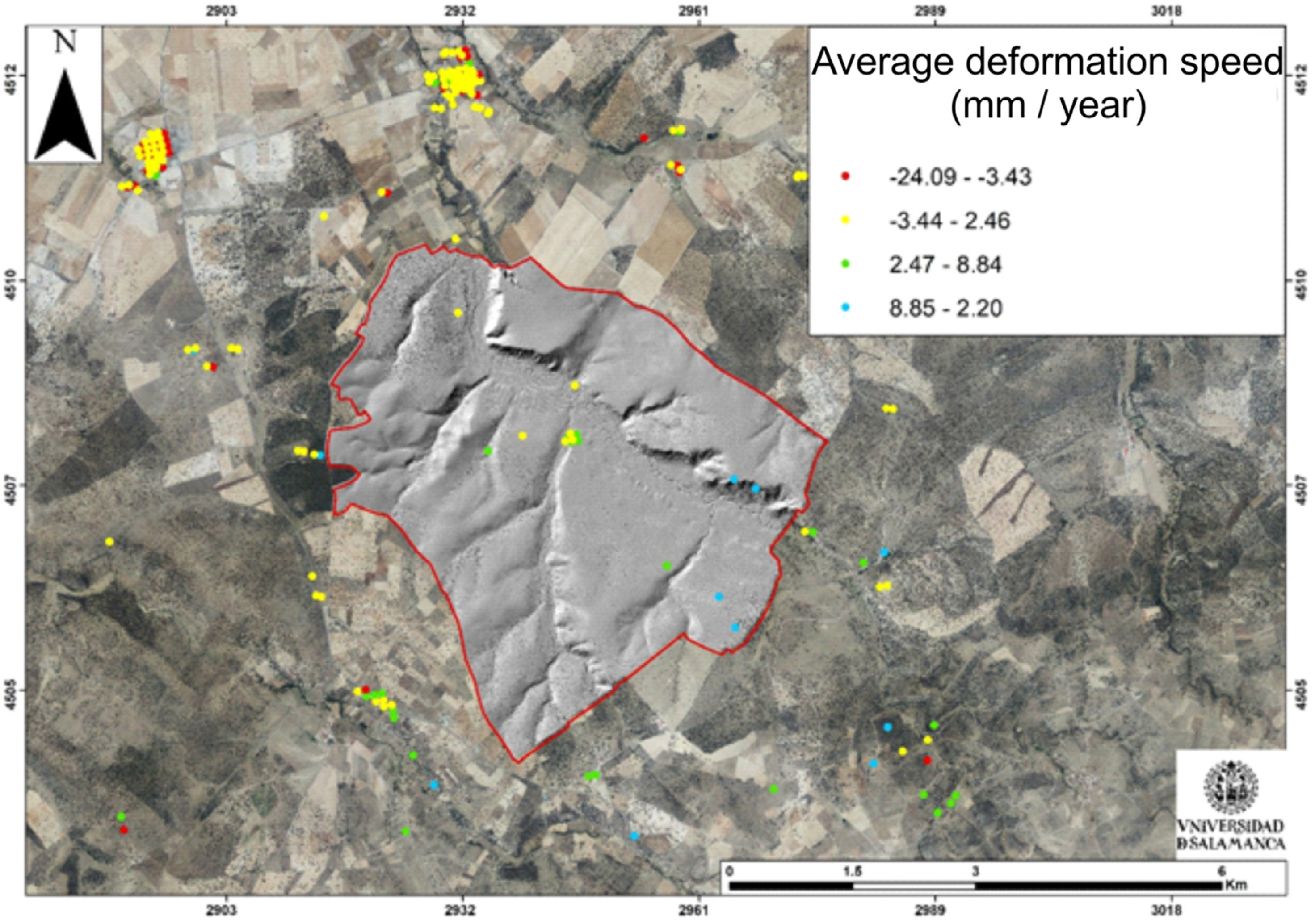
3.1. Analysis of Ground Deformation Velocities (mm/year)

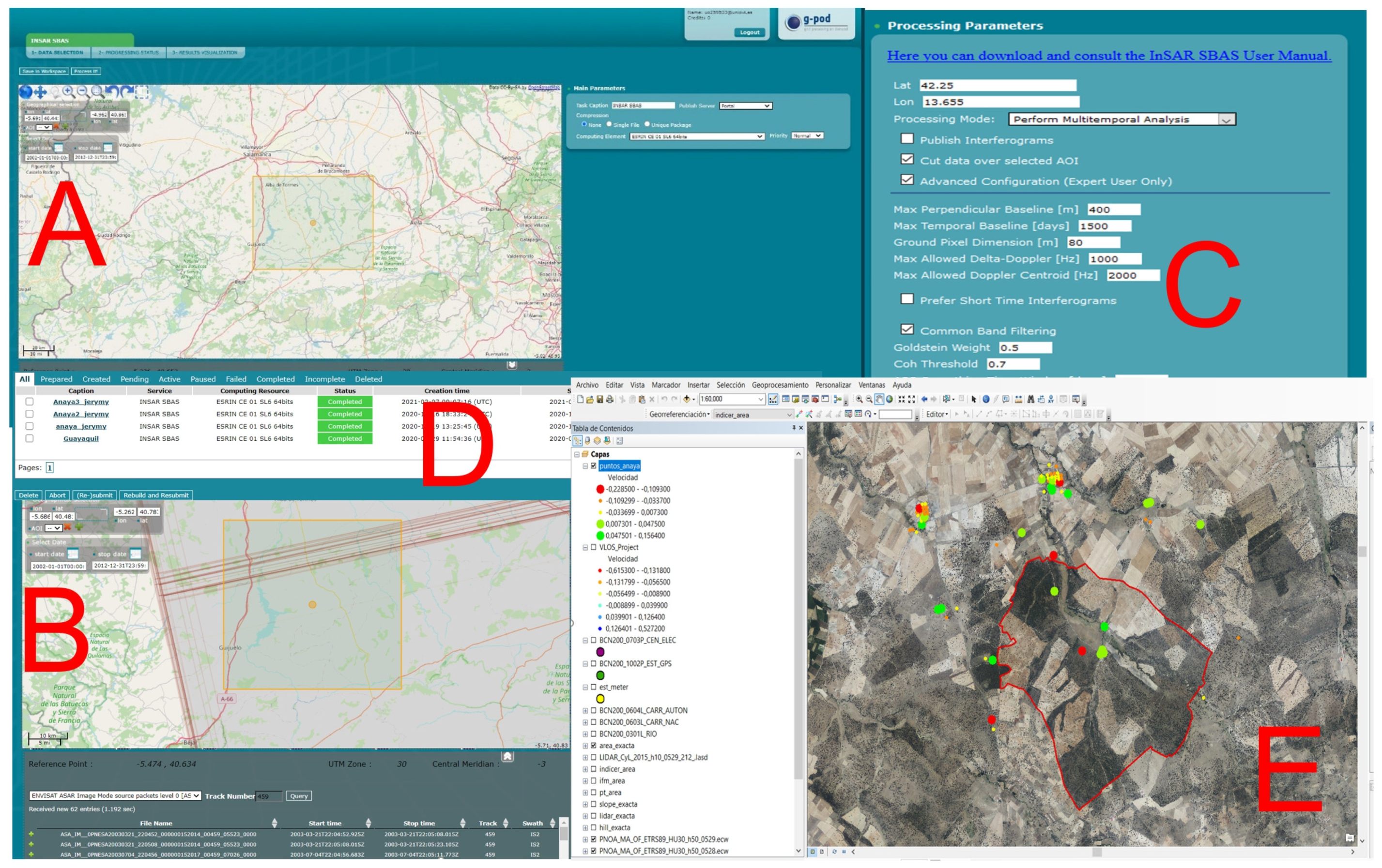
A series of points has been obtained from the application of the A-DInSAR technique of average ground deformation speeds in mm/year (Figure 7). Due to the limitations of the technique, it has been determined that the results obtained from are not valid and/or insufficient because the scale of the study area is too small for the application of tools of this style. In addition, the study area is located in areas with few essential urban reflectors for taking satellite data, which further limits its use. Finally, the presence of dense vegetation accentuates the difficulty of penetrating the satellite laser when collecting data, so this technique definitely contains numerous limitations for this type of study area. In any case, points with average ground velocities of −24.09 mm/year have been found, although very few points have been detected within the perimeter of interest. The positive data found in blue color can indicate the satellite’s approach to the ground, bulging or swelling of the ground or simply atmospheric noise, making this uncertainty invalidate this type of data obtained.

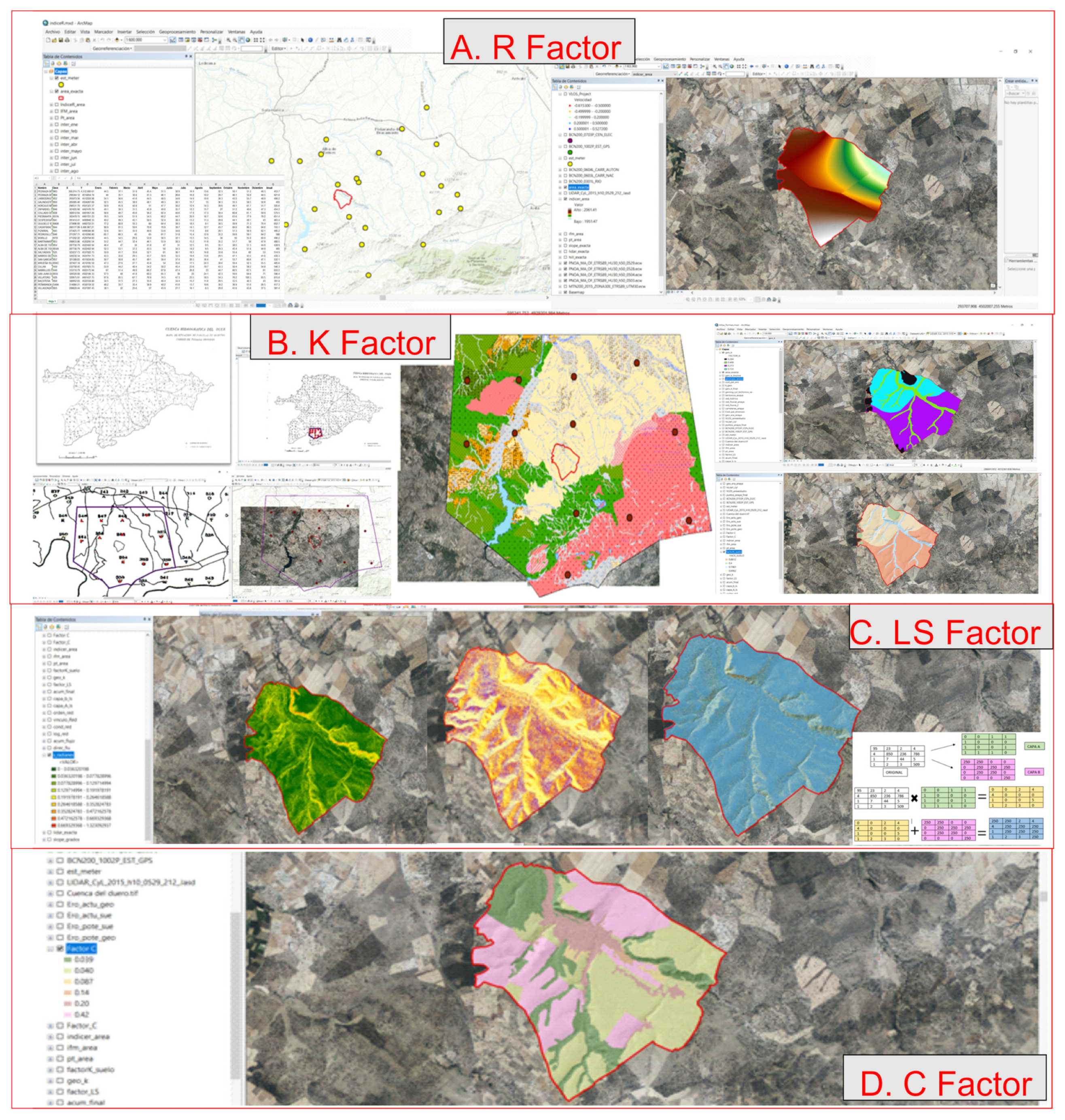
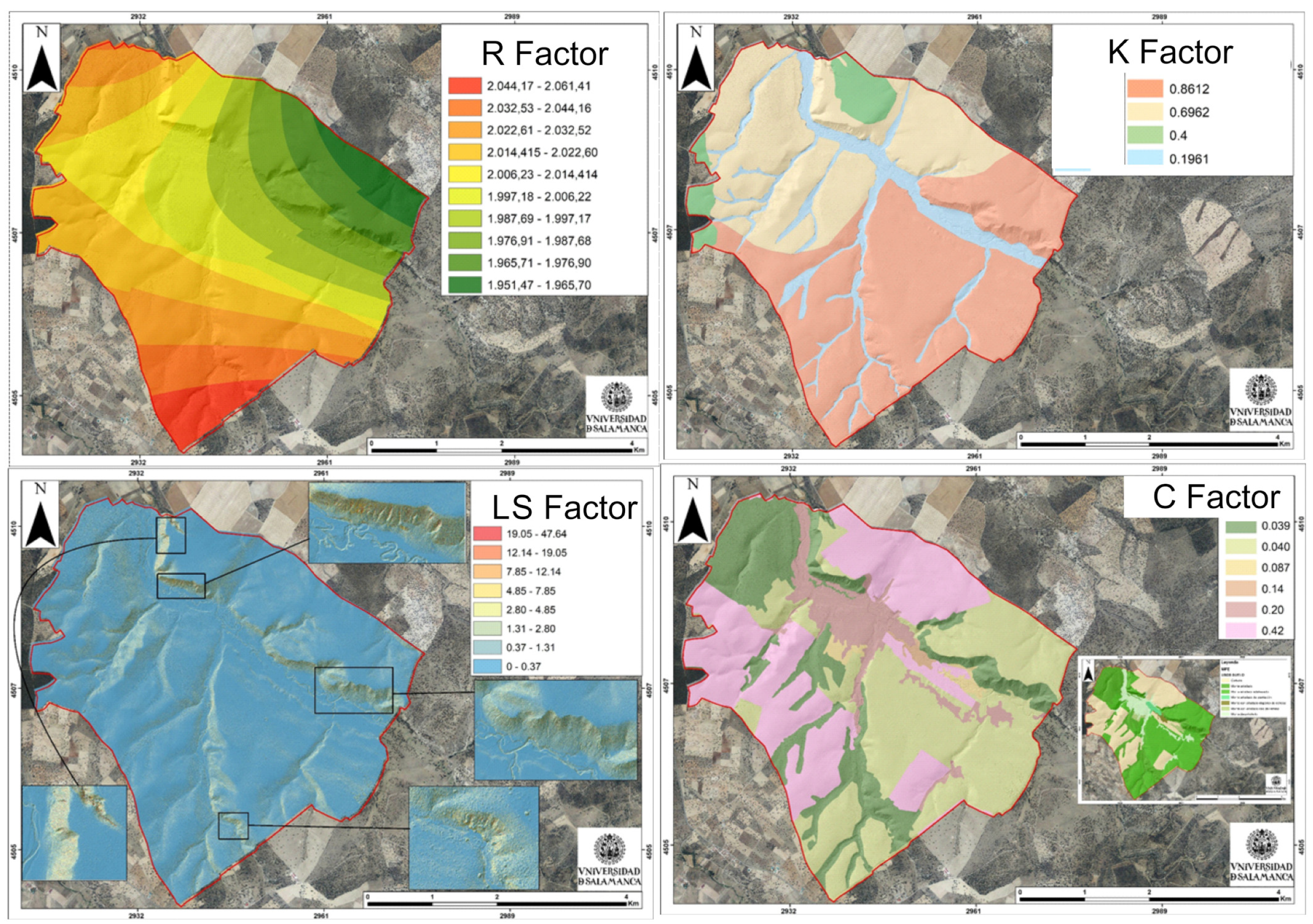
3.2. R Factor or Pluvial Erosivity

It can be seen that the pluvial erosivity values of the study area oscillate between 1951.47 MJ·mm/Ha year–2061.41 MJ·mm/Ha year. There is an increasing trend of the aggressiveness of the rain from the NE zone towards the W-SW, marked by a maximum located in the SW corner where the greatest pluvial erosivity occurs, registered with values in 2061.41 MJ·mm/Ha/year. This maximum is due to the fact that it is positioned on flat areas that contain a gentle slope, causing it to favor the flow of sediments dragged by the water due to precipitation, which the fall impact due to the splash effect easily disintegrates and unstable the sediment of the water ground. On the other hand, the plots with less rainfall erosivity, located to the NE, are located on the flat terraces of the main river, which due to their morphology receive less volume of lateral water and therefore suffer less erosion, since they transport less sediment, some of which can be decanted in times of lower energy, with values between 1.951–1.987 MJ·mm/Ha/year. These types of areas eventually receive rainfall varying its intensity. Ultimately, the key to the R factor is that its increase is due to the presence of areas with steep decline, which favors the flow of water and the dragging of sediment to act as the main erosive factor (Figure 8).

3.3. K Factor or Resistance to Erosion

This factor shows the erodibility or erodibility of the soil from physical properties, considering the lithology (

Table 1. Values of the K factor depending on the lithologies validated for the study area.

Station	Plot	K Factor	Litology
(1) 248A	45.29-SA	0.213	Arcosic sands beige/Arcosic with gravel
(2) 249	45.30-SA	0.284	Gravels at the base and predominant sands with gravels towards top (terraces)
(3) 252A	45.38-SA	0.499	Gravels and feldspathic sands (valley bottoms and floodplains)
(4) 253	45.39-SA	0.133	White coarse arkotic sands with sparse clayey intercalations

W (soil surface mostly with broad-leaved herbaceous plants without plant offal) and G (surface of turf soil with decomposing plant offal at least 2 inches deep).

) and validating our results with the cartography of erosive landscapes of the Duero River hydrographic basin.

This factor is directly related to the geological map of the studied plot, so the resistance to erosion varies depending on the existing lithology. For this specific case, it must be considered that the value of the K factor varies between 0–1, where 0 are conditions more susceptible to erosion and 1 condition are less susceptible to erosion. Values ranging from 0.133 to 0.499 Tm·Ha·h·MJ⁻¹·Ha⁻¹·mm⁻¹ are found, where the zone with the greatest resistance to erosivity is found on the alluvial deposits and valley bottoms since they contain granulometries of clay size which are compacted and adhere, that is, they coalesce, forming a film that is difficult to erode. On the other hand, the most vulnerable areas are those areas with sand-sized granulometries (almost the entire study area, except for the terraces and valley bottoms) which are easily transported by sheets of water causing significant erosion in their wake. The northern area of the study area can be highlighted as the one that suffers the highest soil erosion depending on the rocky substrate with a value of 0.133 Tm·Ha·h·MJ⁻¹·Ha⁻¹·mm⁻¹ as it contains granulometries of coarse sand with ridges, causing greater erosion due to its size. If we consider the existing soils on the lithological substrate and their analytical data of texture and structure from the samplings carried out in the study area. K values vary between 0 (condition least susceptible to erosion) and 1 (condition most susceptible to erosion) contrary to lithology. The resistance to soil erosion contains values ranging from 0.1961 to 0.8612 t·Ha·h·MJ⁻¹·Ha⁻¹·mm⁻¹, fluvisols-type soils being the most resistant to soil erosivity due to the fact that they are cohesive soils, with a greater amount of silts and clays, difficult to erode while passing of a sheet of water, showing values of 0.1961 t·Ha·h·MJ⁻¹·Ha⁻¹·mm⁻¹. On the other hand, the soils located on arches: fundamentally cambisols, are of less resistance to erosion, since they are detrital soils easily eroded by the flow of water, because the sand grains are not connected and are easily transported, being visualized values of 0.6962–0.8612 t·Ha·h·MJ⁻¹·Ha⁻¹·mm⁻¹ (Figure 8).

3.4. LS Factor

Both the length of the slope and its slope influence the erosion rates of the soils in our study area considerably, being the geomorphological aspects related to the forms of the relief one of the main factors that determine the emission of sediments catchment areas. Regarding the length of the slope, it is known the existence of a zone practically without erosion in the highest parts of the slope, the appearance of erosive phenomena of greater intensity in the middle part and sedimentation as the dominant process in the lower part of the slope, where in general its slope decreases. This distribution of erosion occurs in a generalized way on the slopes close to the channels through which the water flows from the study area. Observing the results obtained, it can be seen that soil losses per unit area increase with increasing length of the slope, being greater in its lower part, due to the fact that the runoff sheet accumulates downstream, increasing its drag force as it descends the slope by the action of gravity. On the other hand, on longer slopes the appearance of rills is more frequent, with which erosion rates are considerably increased, as the waters concentrate in these small channels, increasing their speed and transport capacity of the particles eroded soil. The L and S factors are dimensionless and the results obtained vary between 0–47.64, the areas with the greatest erosivity being those with the greatest slope and length of the slope located mainly in the north and northeast of the study area, the existing slopes being that there are between the terraces and the valley bottoms of the main stream. There are also secondary zones with significant erosion potential located to the south and west, caused by secondary channels generated from the main stream (Figure 8).

3.5. C Factor

In our study area, the analysis of the vegetation shows the indicated values (

Table 2. Determination of factor C for arboreal, shrub, mixed wooded formations and herbaceous plant covers.

Arboreal, Shrubby and Mixed Wooded Formations
Cover Type	Type of roof and average drop height of water drip	% Tree and shrub cover	Herbaceous cover and plant offal	% Herbaceous cover and plant offal	C FACTOR
Crops	Trees without low shrub understory (4 m height of fall)	25	W	0	0.42
Wooded mount	Trees without low shrub understory (4 m height of fall)	75	G	60	0.039
Wooded forest pasture	Trees without low shrub understory (4 m height of fall)	50	G	60	0.040
Mount with scattered trees of pasture	Trees without low shrub understory (4 m height of fall)	25	W	40	0.14
Sparse wooded mount of dehesa	Trees without low shrub understory (4 m height of fall)	25	W	60	0.087
Herbaceous Vegetation Covers
Cover Type	% coverage	Establishment or consolidation			C FACTOR
Plantation wooded mount	20	Very poorly			0.20
Treeless mount	20	Very poorly			0.20

). In this factor, stonyness must be considered, which is the proportional decrease in erosion due to the percentage of soil covered by fragments of rock or gravel. Vegetation cover is a determining natural element when studying soil protection against the erosive force of precipitation, since it not only controls the energy with which raindrops reach the soil surface, but also the speed of surface runoff.

The study area is covered mainly by permanent vegetation, causing that the calculated C values are only related to the coverage percentages of the fraction of the room covered by the vegetation, and the herbaceous vegetation, of lower height, varies the protection of the soil throughout the year as a consequence of management (tillage, pruning, etc.) or the development of the plant itself (leaf fall, flowering, etc.). It must be considered that the values of the C factor obtained express the relationship that exists between the annual average soil losses of a plot with a certain vegetation and the losses that that same plot would have under conditions of continuous fallow and tillage according to the maximum slope.

In our sector there is great variability in the values of factor C. The areas where there is a high density of vegetation cover and in contact with the ground, are the areas most resistant to water erosion caused by rainfall, since this cover acts of main protective shield, referring to sectors with values of the C factor of 0.42, 0.20 or 0.14 corresponding to crops, bare forest (formed by grasslands and/or grasslands) and scattered wooded forest of pasture. Being in contact with the ground, the height of fall of the raindrop is lower and therefore contains less erosive energy, which causes greater protection, on the other hand, this type of vegetation obstructs the flow of surface runoff drastically reducing its speed causing it to significantly reduce the erosive power of the water flow, causing the edaphic surface to suffer less damage. In addition, this type of vegetation may have plant remains provided by the existing cover in the study area, which cover the soil and therefore make it more resistant to water erosion, reducing the effect of aggressive rain. On the other hand, the sectors that contain values of the C factor of 0.087, 0.040 and 0.039 corresponding to wooded mountains, wooded forests pastures and wooded forests of thin dehesa formed by hardwood forests and a combination of vegetation mainly, contain less protection against water erosivity due to the fact that they are large vege-tations with crown heights and raindrops falling several meters, making the incidence of rain aggressiveness higher, since the raindrop falls with greater energy accentuating its erosivity. In addition, the speed of the flow of surface runoff through this type of vegetation is higher than in the previous case, since the arboreal permeability and without almost any plant barrier through the soil, cause them to have greater vulnerability to erosion generated by the flow of water.

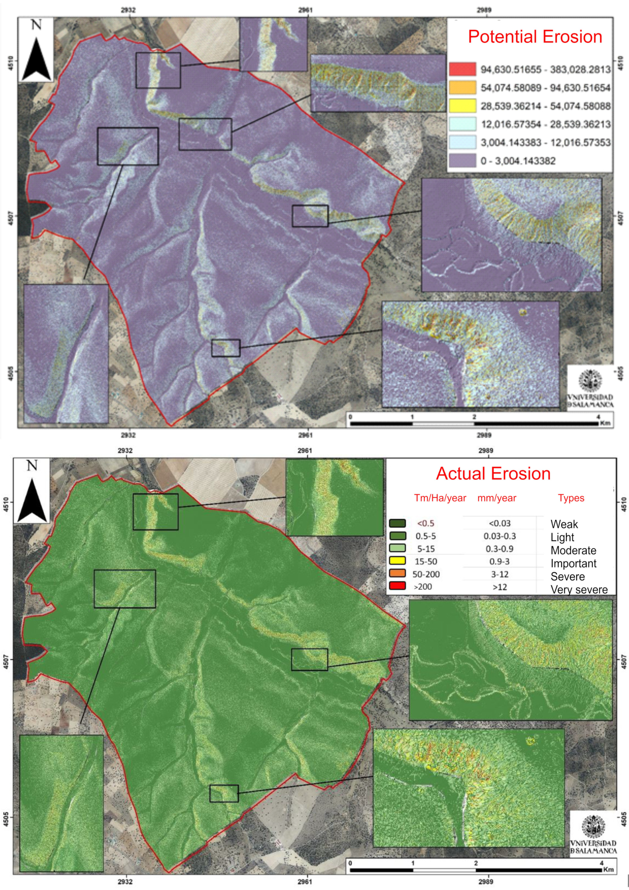
3.6. Potencial Erosión Risk

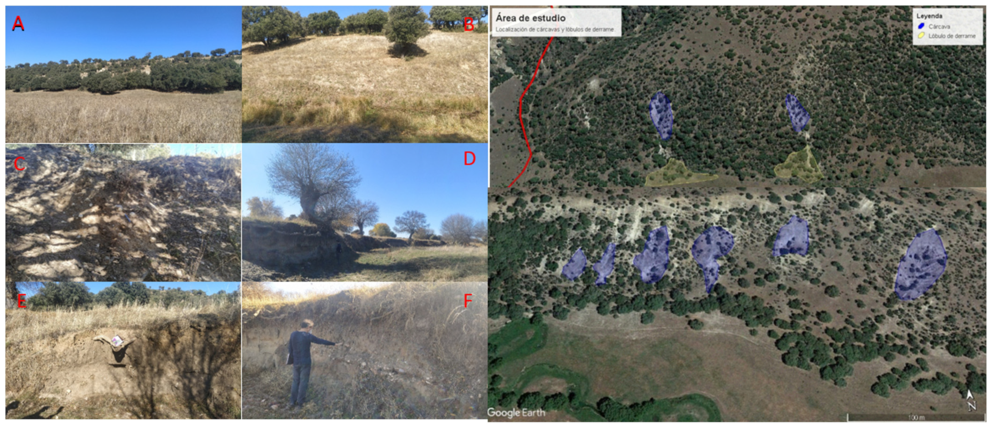
Mapping potential erosion (Figure 9) shows the susceptibility of this area to erosion, considering the existing conditioning factors. To generate the potential risk of soil loss, these factors of the physical environment that condition the erosion processes are multiplied, that is, the factor R, K and LS. Taking these factors into account, it is classified and mapped based on the erodability indices (lithology-soil science and slopes) and erosivity indices (rain aggressiveness). The results in our area show that areas near the main channel (Larrodrigo River) suffer greater processes of water erosion. The main erosive zones are located in the N-NE zone with values of 9,534.735–347,322.90 Tm/Ha/year, leaving certain significant erosive traces such as gullies and even ravines with their associated spill lobes. These areas with high potential for erosion are due to the fact that they contain the steepest slopes of the entire perimeter of interest with the presence of sand-type granulometries, which act as erosive agents when dragged by surface runoff. On the other hand, other areas with significant vulnerability to water erosion are located in secondary tributaries that originate from the main one that are positioned in the south-southwest part of the study area, focusing the erosion on the slopes formed on both sides of These secondary channels, although it contains less intensity due to the presence of a lower slope, exists. In the case of the areas with greater resistance to erosivity, they are distributed throughout almost the entire study area with values ranging between 0–1326.05 Tm/Ha/year, in horizontal flat areas where erosion hardly develops due to to the morphology of the terrain and the little influence that soil erosive agents have. In the field analysis, several videos have been made with drones that show the high degrees of incision of the erosive processes (see video gullies in Supplementary Material) (Supplementary Materials: Video S1: Badlands-gullies).

3.7. Actual Erosion Risk

In this section, the current erosion risk is analyzed and mapped (Figure 9), starting from the potential erosion risk and subtracting the protection offered by the vegetative cover based on its characteristics (height, density, stratification and spacing). territorial). The classification of the degrees of water erosion obtained with these thematic cartographies is regrouped in the intervals established by the Food and Agriculture Organization of the United Nations (FAO) expressed in Tm/Ha/year and mm/year.

The results of the current erosion show that the areas that suffer the greatest processes of water erosion fall mainly in areas close to the main stream that runs from top to bottom in the study area (Larrodrigo river), with current water erosion ranging from important- moderate to very severe or irreversible with values ranging between 5 → 200 Tm/Ha/year with soil losses ranging between 0.3 → 12 mm/year, mainly differentiating the N-NE and S-SW sectors of the study zone. These are sectors that contain high slopes where surface runoff flows at high speed, dragging sand and gravel, causing intense erosion and incision in its path. In addition, they contain vegetation that has little protective power, since they are wooded mountains with multi-meter crowns with hardly any vegetation on bare soils, further accentuating their erosive vulnerability. The rest of the study area corresponds to areas with great resistance to erosivity, since the morphology of its terrain with absence of slope, finer granulometries such as clays and its vegetation in contact with the ground makes it well protected to water erosion caused by rainfall, with values of <0.5–5 Tm/Ha/year with losses of >0.03–0.3 mm/year mainly, being a weak and/or slight soil loss.

4. Conclusions

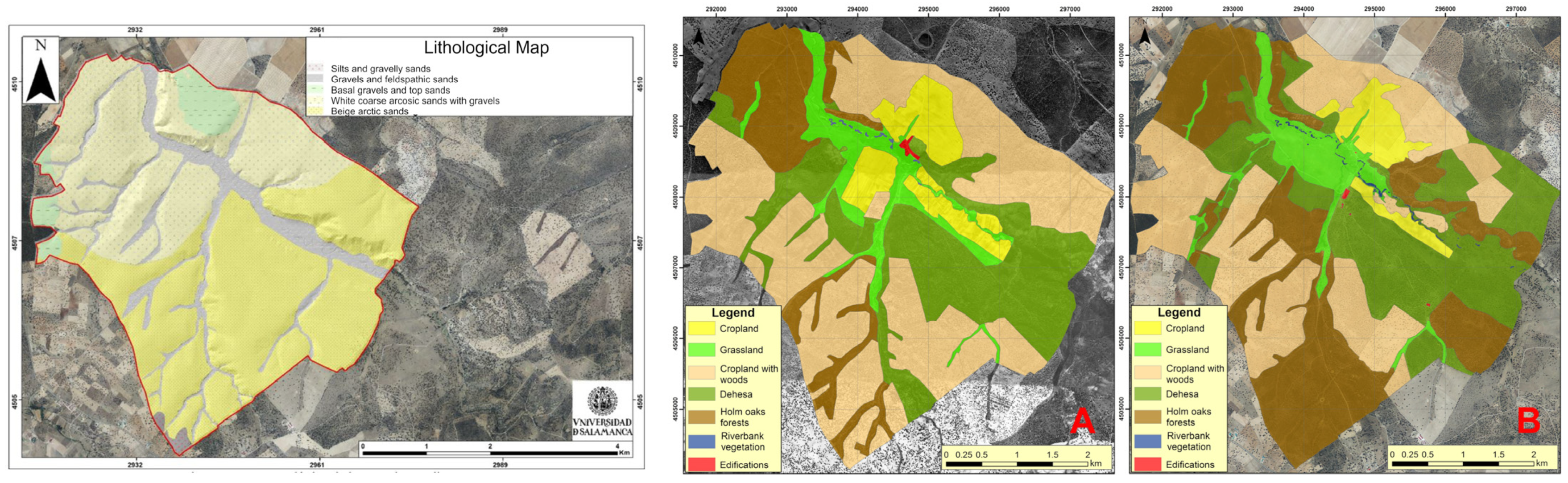
The modeling and automation of the RUSLE model with GIS allows a detailed and exhaustive multiparametric analysis that facilitates the analysis of the risk of water erosion in any territory where active processes are produced by sediment movements. The generation of a geodatabase, based on the determining components of the territory, has allowed obtaining the potential and actual erosion maps, being able to establish the volume of the problem in the study area, in such a way that soil losses are calculated and quantified by water erosion. Simultaneously, the combined use of A-DInSAR and GIS techniques was used to identify the possible movements of the sediment from differences between satellite images and observing the deformation speedb of the terrain associated with mass movements due to instability of slope and subsidence phenomena within the study area. It has clearly been shown that the use of this type of DInSAR techniques linked to the size or scale of the study area are not compatible when it comes to obtaining valid and consistent results, being more accurate in larger areas and where there is a greater number of receivers or urban helmets essential for taking satellite data. Two different sectors are defined by their erosive degree. The first presents levels that go from moderate to very serious or irreversible with values that oscillate between 5 → 200 Tm/Ha/ year with losses of the land of 0.3 → 12 mm/year. This sector corresponds to areas near the Larrodrigo river, encompassing the slopes that connect with the terraces positioned to the N and NE of the study area, with a high degree of water erosivity due to the presence of very high slopes and where the vegetation is scarce, generating erosive forms of great incision in the land (gullies) that put at risk the sustainable livestock and agricultural activity of this sector. The other sector corresponds to secondary channels perpendicular to the main one, located in the W and SW part.

According to the erosion rates observed among the different land uses, it should be noted that the main conversions in land use occurred between croplands with trees and open areas of pasture, which became holm oaks with dense areas shrubs, mainly the result of the lack of forest management, being observable in the southern and western areas of the studied sector. As a result, the current rate of erosion on the farm is lower due to the protection that the holm oaks and permanent pasture provide to the soil. The open areas dedicated to cultivation have higher rates than the holm oaks. On the other hand, the prairie areas present low rates of erosion, similar to holm oaks, the result of the dense herbaceous cover that covers them.

However, particularizing within each type of land cover, important differences were observed. The case for the use of the land of holm oaks stands out, in which erosion rates are usually minimal due to the protection provided by the vegetation and the smooth orography in which they are usually found. However, the wooded areas on the right bank of the Larrodrigo stream (also observable on a smaller scale in other smaller streams), with predominant land use of holm oaks, present the highest erosion rates, so the use of the soil Holm oak brings together the upper and lower extreme values of the erosion rate on the farm. These high rates of erosion in the escarpment areas are mainly due to their steep slope, which is further enhanced by a significant absence of herbaceous vegetation due to the absence of fertile soil, the loss of which has been accelerated by the trampling of the cattle found here over time.

The cartography of the potential and current erosion risk of water erosion allows to establish in a simple way, as applied in the methodology presented in this article, the classes of degrees of erosion obtained according to the FAO, expressed in Tm/Ha/year and mm/year. This thematic mapping constitutes in itself a low-cost non-structural measure that helps to identify the areas or sectors where the implementation of a soil management and conservation plan is necessary and urgent, such as management in the change of land use. land and reforestation, as well as detecting restoration measures and adaptation of land uses. In addition, it is possible to identify areas with high rates of sediment production that constitute areas susceptible to edaphic loss and to determine the location of sediment retention structures and other measures determining the true effect on anthropic activities of first need since the Soil is a resource that is difficult to remove at the speed with which it is lost, as shown in the ratios of the cartographies carried out.

References

1. Nájera González, O.; Bojórquez Serrano, J.I.; Flores Vilchez, F.; Murray Núñez, R.M.; Areli González García-Sancho, A. Riesgo de erosión hídrica y estimación de pérdida de suelo en paisajes geomorfológicos volcánicos. En México. Ministerio de Educación Superior. Cuba Instituto Nacional de Ciencias Agrícolas. Cultiv. Trop. 2016, 37, 45–55. [Google Scholar]
2. Morgan, R.P.C. Erosión y Conservación del Suelo; Ediciones; Mundi-Prensa: Madrid, Spain, 1997; 354p. [Google Scholar]
3. Morgan, R.P.C. A simple approach to soil loss prediction: A revised Morgan–Morgan–Finney model. Catena 2001, 44, 305–322. [Google Scholar] [CrossRef]
4. Martínez-Graña, A.M.; Goy, J.L.; Zazo, C. Cartographic procedure for the analysis of eolian erosion hazard in Natural Parks (Central System, Spain). Land Degrad. Dev. 2015, 26, 110–117. [Google Scholar] [CrossRef]
5. Lal, R.; Sobecki, T.M.; Iivari, T.; Kimble, J.M. Soil Degradation in the United States. Extent, Severity and Trends. Lewis Publ. 2003, 204, 5–9. [Google Scholar]
6. FAO. Erosion de suelos en américa Latina. In Proceedings of the Taller Sobre la Utilización de un Sistema de Información Geográfica (SIG) en la Evaluación de la Erosión Actual y de Suelos y la Predicción del Riesgo de Erosión Potencial. Santiago, Chile, 27 June–1 August 1992. 1993 92--3001-5. [Google Scholar]
7. Gustavsson, M.; Kolstrup, E.; Seijmonsbergen, A.C. A new symbol-and-GIS based detailed geomorphological mapping system: Renewal of a scientific discipline for understanding landscape development. Geomorphology 2006, 77, 90–111. [Google Scholar] [CrossRef] [Green Version]
8. Martinez-Grana, A. Estudio Geológico Ambiental Para la Ordenación de LOS espacios Naturales de “las Batuecas-Sierra de Francia”. Aplicaciones Geomorfológicas al Paisaje, Riesgos e Impactos; Universidad de Salamanca: Salamanca, Spain, 2010. [Google Scholar]
9. Ferretti, A.; Prati, C.; Rocca, F. Permanent scatterers in SAR interferometry. IEEE Trans. Geosci. Remote Sens. 2001, 39, 8–20. [Google Scholar] [CrossRef]
10. Berardino, P.; Fornaro, G.; Lanari, R.; Sansosti, E. A new algorithm for surface deformation monitoring based on small baseline differential sar interferogram. IEEE Trans. Geosci. Remote Sens. 2002, 40, 2375–2383. [Google Scholar] [CrossRef] [Green Version]
11. Mora, O.; Mallorquí, J.J.; Broquetas, A. Linear and nonlinear terrain deformation maps from a reduced set of interferometric SAR images. IEEE Trans. Geosci. Remote Sens. 2003, 41, 2243–2253. [Google Scholar] [CrossRef]
12. Sánchez-Sánchez, Y.; Martínez-Graña, A.; Santos-Francés, F. Remote Sensing Calculation of the Influence of Wildfire on Erosion in High Mountain Areas. Agronomy 2021, 11, 1459. [Google Scholar] [CrossRef]
13. Casu, F. SBAS-DInSAR Parallel Processing for Deformation Time-Series Computation. IEEE J. Sel. Top. Appl. Earth Obs. Remote Sens. 2014, 7, 3285–3296. [Google Scholar] [CrossRef]
14. Herrera, G.; Tomás, R.; López-Sánchez, J.M.; Monserrat, O.; Cooksley, G.; Mulas, J. Sistemas radar aplicados a la investigación de subsidencia y movimientos de ladera. Enseñanza de las Ciencias de la Tierra 2009, 17, 316–324. [Google Scholar]
15. Barra, A.; Solari, L.; Béjar-Pizarro, M.; Monserrat, O.; Bianchini, S.; Herrera, G.; Crosetto, M.; Sarro, R.; González-Alonso, E.; Mateos, R.M.; et al. A methodology to detect and update active deformation areas based on sentinel-1 SAR images. Remote Sens. 2017, 9, 19. [Google Scholar] [CrossRef] [Green Version]
16. Martinez-Graña, A.; Goy, J.; Zazo, C. Dominant soil map in ‘Las Batuecas-Sierra De Francia’ and ‘Quilamas’ nature parks (Central System, Salamanca, Spain). J. Maps 2014, 11, 371–379. [Google Scholar] [CrossRef]
17. Instituto Geológico Minero de España (IGME). Mapa Geológico de España 1:50.000. Alba de Tormes; Segunda Serie-Primera Edición; Ministerio de Industria y Energía: Madrid, Spain, 1982. [Google Scholar]
18. Instituto Geológico Minero de España (IGME). Mapa Geológico de España 1:50.000. Santa María del Berrocal; Ministerio de Industria y Energía: Madrid, Spain, 2008; ISBN 978-84-7840-747-7. [Google Scholar]
19. Wischmeier, W.H.; Smith, D.D. Predicting Rainfall Erosion Losses: A Guide to Conservation Planning; No. 537; Department of Agriculture, Science and Education: College Park, MD, USA, 1978. [Google Scholar]
20. Borrelli, P.; Alewell, C.; Alvarez, P.; Anache, J.A.A.; Baartman, J.; Ballabio, C.; Bezak, N.; Biddoccu, M.; Cerdà, A.; Chalise, D.; et al. Soil erosion modelling: A global review and statistical analysis. Sci. Total. Environ. 2021, 780, 146494. [Google Scholar] [CrossRef] [PubMed]
21. González del Tánago, M. La Ecuación Universal de Perdidas de Suelo. Pasado, Presente y Futuro. Ecología, n. 5; ICONA: Madrid, Spain, 1991; pp. 13–50. [Google Scholar]
22. Wischmeier, W.H. Use and Misuse of The Universal Soil Loss Equation. J. Soil Water Conserv. 1976, 31, 5–9. [Google Scholar]
23. Van der Knijff, J.M.; Jones, R.J.; Montanarella, L. Soil Erosion Risk Assessment in Europe; European Commission: Florence, Italy, 2000; p. 52. Available online: https://esdac.jrc.ec.europa.eu/content/soil-erosion-risk-assessment-italy (accessed on 20 October 2021).
24. Panagos, P.; Ballabio, C.; Poesen, J.; Lugato, E.; Scarpa, S.; Montanarella, L.; Borrelli, P. A Soil Erosion Indicator for Supporting Agricultural, Environmental and Climate Policies in the European Union. Remote Sens. 2020, 12, 1365. [Google Scholar] [CrossRef]
25. Garcia-Ruiz, J.M.; Lopez Bermudez, F. La Erosión del Suelo en España; Sociedad Española de Geomorfología (SEG), Ed.; Sdad. Coop. de Artes Gráficas: Zaragoza, Spain, 2009; ISBN 978-84-692-4599-6. [Google Scholar]
26. Flacke, W.; Auerswald, K.; Neufang, L. Combining a modified Universal Soil Loss Equation with a digital terrain model for computing high resolution maps of soil loss resulting from rain wash. Catena 1990, 17, 383–397. [Google Scholar] [CrossRef]
27. Meusburger, K.; Konz, N.; Schaub, M.; Alewell, C. Soil erosion modelled with USLE and PESERA using QuickBird derived vegetation parameters in an alpine catchment. Int. J. Appl. Earth Obs. Geoinf. 2010, 12, 208–215. [Google Scholar] [CrossRef]
28. Khaleghpanah, N.; Shorafa, M.; Asadi, H.; Gorji, M.; Davari, M. Corrigendum to “Modeling soil loss at plot scale with EUROSEM and RUSLE2 at stony soils of Khamesan watershed, Iran” [Catena (147C) (2016) 773–788]. Catena 2017, 151, 259. [Google Scholar] [CrossRef]
29. Gholami, V.; Booij, M.; Tehrani, E.N.; Hadian, M. Spatial soil erosion estimation using an artificial neural network (ANN) and field plot data. Catena 2018, 163, 210–218. [Google Scholar] [CrossRef]
30. Renard, K.G.; Foster, G.R.; Weesies, G.A.; McCool, D.K.; Yoder, D.C. Predicting Soil Erosion by Water: A GUIDE TO COnservation Planning with the Revised Universal Soil Loss Equation (RUSLE); US Government Printing Office: Washington, DC, USA, 1997; Volume 703. [Google Scholar]
31. Moore, I.D.; Burch, G.J. Physical Basis of the Length-slope Factor in the Universal Soil Loss Equation. Soil Sci. Soc. Am. J. 1986, 50, 1294–1298. [Google Scholar] [CrossRef]
32. Sanchez, Y.; Martínez-Graña, A.; Santos-Francés, F.; Yenes, M. Influence of the sediment delivery ratio index on the analysis of silting and break risk in the Plasencia reservoir (Central System, Spain). Nat. Hazards 2018, 91, 1407–1421. [Google Scholar] [CrossRef]
33. Terranova, O.; Antronico, L.; Coscarelli, R.; Iaquinta, P. Soil erosion risk scenarios in the Mediterranean environment using RUSLE and GIS: An application model for Calabria (southern Italy). Geomorphology 2009, 112, 228–245. [Google Scholar] [CrossRef]
34. AbdulKadir, T.S.; Muhammad, R.M.; Khamaruzaman, W.Y.; Ahmad, M.H. Geo-statistical based susceptibility mapping of soil erosion and optimization of its causative factors: A conceptual framework. J. Eng. Sci. Technol. 2017, 12, 2880–2895. [Google Scholar]
35. Esteves, T.; Kirkby, M.; Shakesby, R.; Ferreira, A.; Soares, J.; Irvine, B.; Ferreira, C.; Coelho, C.; Bento, C.; Carreiras, M. Mitigating land degradation caused by wildfire: Application of the PESERA model to fire-affected sites in central Portugal. Geoderma 2012, 191, 40–50. [Google Scholar] [CrossRef]
36. Martínez-Graña, A.M.; Goy, J.L.; Zazo, C. Water and wind erosion risk in natural parks. A case study in “Las Batuecas-Sierra de Francia” and “Quilamas” protected parks (Central System, Spain). Int. J. Environ. Res. IJER 2014, 8, 61–68. [Google Scholar]
37. Alcañiz, J.M. Erosión: Evaluación del Riesgos Erosivo y Practicas de Protección del Suelo; Universidad de Girona: Girona, Spain, 2008; ISBN 978-8496742-37-6. [Google Scholar]
38. Lal, R. Soil Erosion and the Global Carbon Budget; School of Natural Resources, The Ohio State University: Columbus, OH, USA, 2002. [Google Scholar]
39. Martinez-Graña, A.; Goy, J.L.; Cruz, R.; Forteza, J.; Zazo, C.; Barrera, I. Cartografía Del Riesgo De Erosión Hídrica Mediante SIG En Los Espacios Naturales De Candelario–Gredos (Salamanca, Avila). Edafología 2006, 13, 11–20. [Google Scholar]
40. Ganasri, B.; Ramesh, H. Assessment of soil erosion by RUSLE model using remote sensing and GIS—A case study of Nethravathi Basin. Geosci. Front. 2016, 7, 953–961. [Google Scholar] [CrossRef] [Green Version]
Figure 1. Situation map of Study area (left). The satellite image (right) shows the great importance of the conservation of the arboreal roots (dark green areas) scattered throughout a region in which bare soils are abundant (light brown color).
Agronomy 11 02120 g001
Figure 2. Left. Geological Map. Right: Changes in land use observed in the study area: 1956 (A) and 2020 (B) based on SIOSE (https://www.siose.es/) (accessed 20 October 2021).
Agronomy 11 02120 g002
Figure 3. Workflow.
Agronomy 11 02120 g003
Figure 4. Left. (A): Overview of spill cones associated with gullies. (B): Detail of front of fans. (C): Erosive tracks due to sediment flow. (D): Contrast of vegetation present in the study area. (E): Visualization of the material carried by the water flow. (F): Detail photo corresponding to (E). Right. Location in Google Earth of erosive marks such as gullies and their associated spill lobes.
Agronomy 11 02120 g004
Figure 5. (A). Selection of the study area for the subsequent search and processing of SAR images. (B). Choice of the track number and display of the images to be processed. (C) Parameters chosen for image processing. (D). Process control and processing status. (E) Displacement mapping obtained in the study area.
Agronomy 11 02120 g005
Figure 6. Calculation procedures for R factor (File A), K factor (File B), LS factor (File C) and C factor (File D).
Agronomy 11 02120 g006
Figure 7. Cartography of mean deformations of the terrain indicating with colors the different speeds obtained from the satellite difference analyzed between images.
Agronomy 11 02120 g007
Figure 8. Cartographies obtained from the different factors of the RUSLE in the study area (red border line).
Agronomy 11 02120 g008
Figure 9. Cartographies with the distribution of the potential erosion risk expressed in Tm/Ha/year (Top) and the actual erosion risk (Bottom).
Agronomy 11 02120 g009