Understanding the Temporal Variability of Rainfall for Estimating Agro-Climatic Onset of Cropping Season over South Interior Karnataka, India

Abstract

Annual, seasonal and intra-seasonal variations in rainfall affect crop production from land preparation to the realization of potential crop yield in a region. Particularly, the onset of the rainy season is most crucial for determining the sowing period. Statistical analysis (Modified Mann-Kendall aka MMK-test for trend and likelihood ratio test for shifting pattern) of 60 years rainfall of south interior Karnataka (SIK) inferred the presence of temporal variability in rainfall. There was a monotonic increase in rainfall of February, March, April, June and August months (a positive sign of MM-K (tau) value), with a negligible rate of change (Sen’s slope towards zero). Upon seasonal analysis, there was a significant increase in winter, pre-monsoon and monsoonal rainfall as compared to post-monsoonal rainfall (higher Sen’s slope for pre-monsoon), indicating a need for agronomic interventions for estimating an effective date of sowing for reducing risks of crop production. Further, the agro-climatic onset of cropping season was estimated by considering soil–crop–water relations. Earlier onset of cropping season was estimated based on thresholds of soil–crop–water relations, which highlights sowing of crops in advance (May 1st fortnight) instead of late (June 1st fortnight) to avoid crop losses due to early-season drought.

1. Introduction

Among several features of monsoonal regions of the world, seasonal variation of rainfall is the most distinguishing. About 80% of the annual rainfall in India occurs during the summer monsoon period, June–September [1]. The year-to-year variability in monsoon rainfall occasionally leads to extreme hydrological events (large-scale droughts and floods), resulting in a serious reduction in agricultural output and affecting the vast population (in excess of one billion) and the national economy [2]. A normal monsoon with an evenly distributed rainfall throughout the country is a bonanza, while an extreme event of flood or drought over the entire country or a smaller region constitutes a natural hazard. Hence the variation in seasonal monsoon rainfall may be considered a measure to examine climate variability/change over the Indian monsoon domain in the context of global warming [3].

Rainfall plays a dominant role in agricultural production and productivity, despite advancement in many technological fronts. The fourth assessment report (AR4) of the Inter-governmental Panel on Climate Change (lPCC) (2007) [4] indicated with very high confidence (90% probability of being correct) that human activities, since industrialization, have caused the planet to warm by about 1 °C and future climate change is likely to affect agriculture and increase the risk of hunger and water scarcity [5]. The intra-annual, inter-seasonal and intra-seasonal rainfall variations affect agriculture from land preparation to the realization of the potential yield of crops [6], and seasonal changes in rainfall patterns may alter the cropping pattern and cropping system [7].

Many attempts for prediction of monsoon onset have been made for different time scales using numerical prediction models [8]. Forecasting methods have so far been mostly based on statistical model approaches, which include averaged values of zonal asymmetric temperature anomaly [9], sea surface temperature, mean sea level pressure [8,10], tropospheric moisture buildup over areas south of the Indian peninsula [11], vertically integrated moisture budget (hydrologic onset and withdrawal index) [12], moist static energy [13], outgoing longwave radiation (OLR), wind fields [14] and, recently, critical transition precursor-based methods considering precipitation along with air temperature and relative humidity were considered to estimate the onset and withdrawal [15]. However, there are certain difficulties in the existing forecasting methods, in particular, of false monsoon onsets mostly related to non-monsoonal atmospheric circulation systems [16]. These limitations require improvements in the prediction skills for monsoon onset.

The subject area of climate change is vast; the changing pattern of rainfall is a topic within this field that deserves urgent and systematic attention since it affects both the availability of fresh water and food production [17]. Higher the rainfall or lower the rainfall or changes in its spatial and seasonal distribution would influence the spatial and temporal distribution of runoff, soil moisture and groundwater reserves and would affect the frequency of droughts and floods. Unlike irrigated agriculture, rainfed farming is usually diverse and risk-prone. Small variations in the timing and the quantity of rainfall have a potential impact on agricultural output [18]. Among the states, Karnataka is facing frequent drought conditions due to uncertainty in rainfall and spatiotemporal variation in different regions.

Due to these variations in rainfall distribution, Karnataka is experiencing extreme weather conditions such as drought or flood in different regions. Frequent drought and floods have caused heavy loss to crops and lives, while society loses its livelihood and rhythm of life, and people are forced to migrate for their sustenance. As rainfall is an unpredictable natural phenomenon, statistical analysis of its distribution patterns and quantum of rainfall plays an important role [19]. The statistical analysis of rainfall paves the way for help the government in agricultural planning and policymaking and for farmers in adopting the farm production practices, crop contingency planning, etc. [20].

In southern Karnataka, major soil types are sandy clay, some drought-tolerant crops such as pigeonpea, finger millet, sugarcane etc., are grown, but local varieties are not very productive. These low yields and their high variability, combined with the fast demographic increase, are the main cause of recurrent food crises. Many reasons explain the weakness and spatiotemporal variability of crop yields in these regions. One of the most important risk factors is the high spatial and temporal variability of rainfall across the region [21]; this is exacerbated by poor soil fertility [22]. The rainy season lasts from April to November and receives between 528 to 1374 mm of rainfall (average 914). Several climatic factors such as seasonal rainfall amount, intra-seasonal rainfall distribution and dates of onset/cessation of the rains influence crop yields and determine the agricultural calendar [23,24]. In particular, the onset of the rainy season appears to be the most crucial information for agricultural management [25,26] since it determines the planting period [27,28,29]. Traore et al. (2007) [30] emphasized differences between agro-climatic and farmers’ definitions of the onset of the rains. The agro-climatic approach defines the onset as the optimal date that ensures sufficient soil moisture during planting and early growing periods to avoid crop failure after sowing [23,29,31,32].

Traditionally, sowings begin as early as possible and coincide with the first substantial rainy event [33], which occurs generally around one month before the full establishment of the monsoon [34]. Since the monsoon season has not begun yet, the probability of a post-sowing dry spell is high, increasing the risk of a sowing failure. Farmers balance this risk, inducing a loss of seeds and an increase of labor devoted to re-sowing, with the beneficial nitrogen flush associated with the first rains [35,36,37]. Moreover, late sowings not only miss this flush but also shorten the growing season and increase weed pressure and weeding [38,39,40]. In this paper, an attempt is made to illustrate how rainfall determines the choice of sowing date and evaluates the relationship between sowing and onsets dates defined using agro-climatic approaches.

2. Materials and Methods

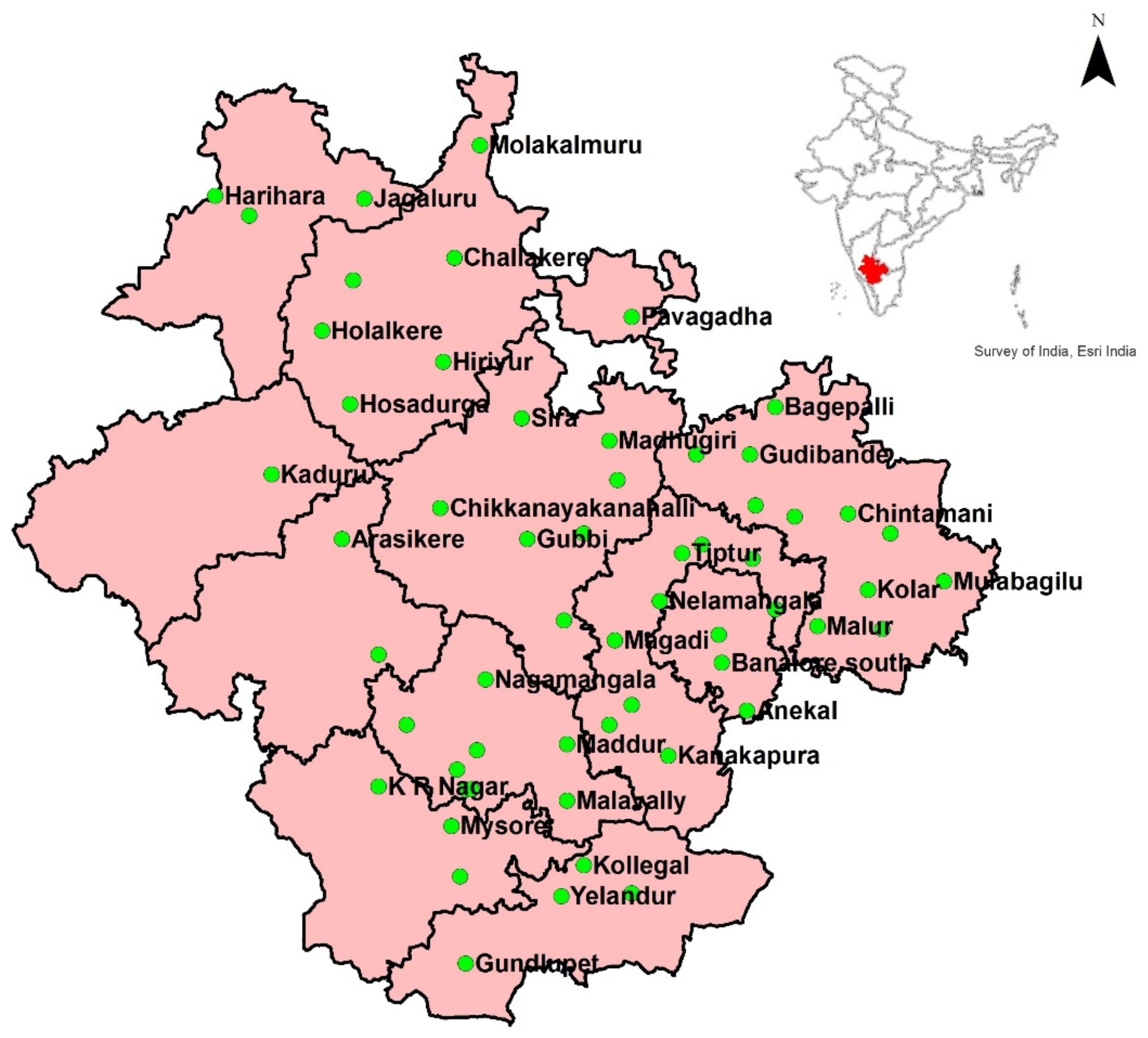
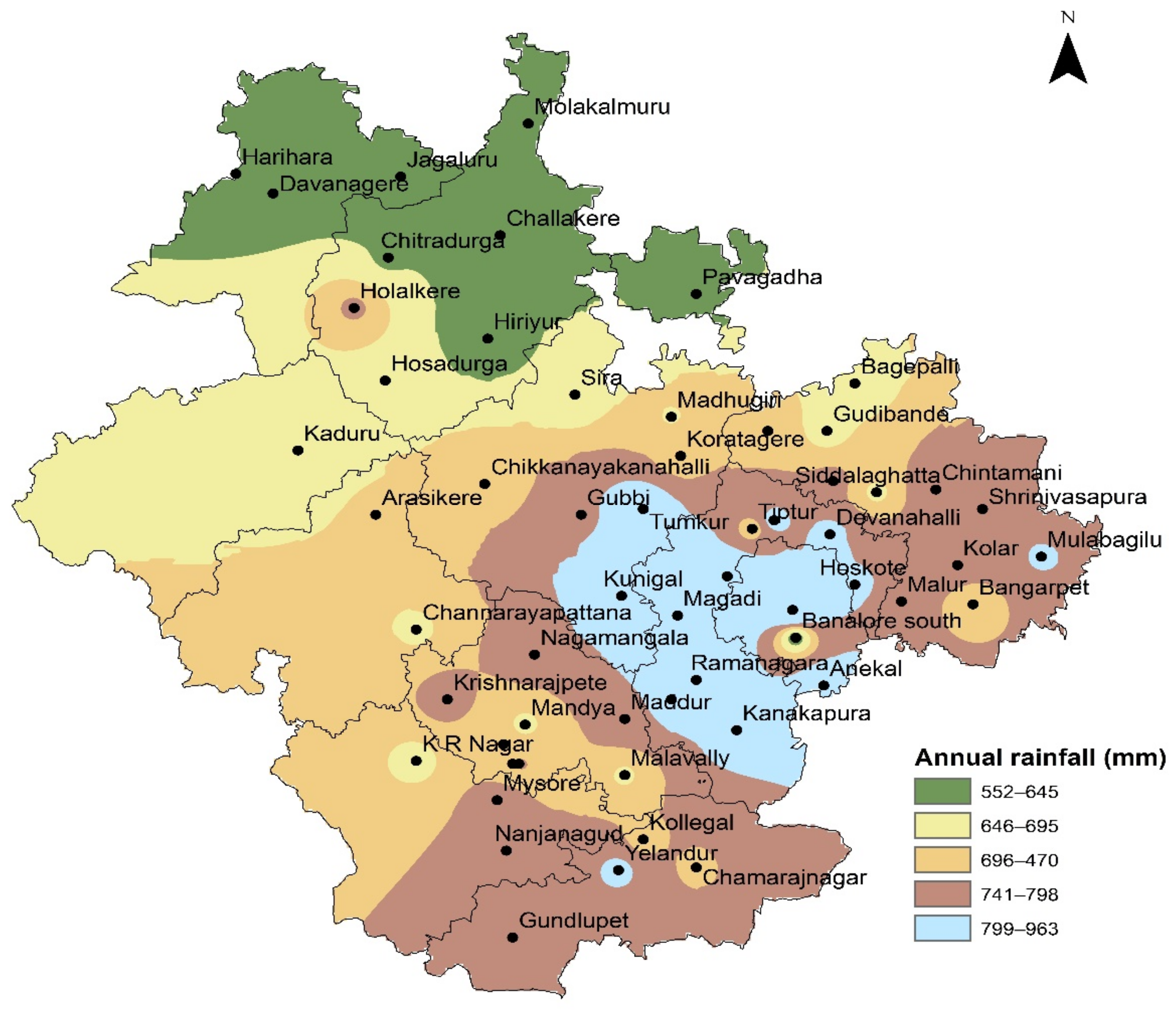
2.1. Study Area

Karnataka (located between 11.40°–18.27° N latitudes and 74.25°–78.50° E longitudes and covers an area of 19.1 M. Ha that accounts for 5.8% of the total area of the country) has tropical monsoon characterized by hot and moist summers and cool and dry winters [21]. There is a diversity in the climate of the state, influenced by geographical location, oceans, physical features, vegetation and monsoon winds. Hence, the annual temperature and distribution of rain are not the same all over the state. The state has a net cultivated area of 10.5 M Ha, net irrigated area of 3.49 M Ha and net rainfed area of 7.01 M ha [41].

Based on the common rainfall distribution pattern, Karnataka state is classified into four meteorological subdivisions, namely North Interior Karnataka (NIK), South Interior Karnataka (SIK, 13.18°–13.32° E and 75.82°–76.59° N), Coastal subdivision and Malnad subdivision. The study area, i.e., SIK subdivision, comprises 11 districts (

Table 1. Districts and blocks of SIK from where rainfall data was collected.

Zone	District	Blocks (Location of Rain Gauge)
CDZ	Chitradurga	Chitradurga, Hosadurga, Challakere, Molakalmuru, Holalkere, Hiriyuru
	Davanagere	Davanagere, Harihara, Jagaluru
	Tumakuru	Madhugiri, Pavaghadha, Sira, Chikkanayakanahalli
	Chikkamagaluru	Kaduru
EDZ	Tumakuru	Gubbi, Koratagere
	Bangalore (rural)	Devanahali, Doddaballapura, Nelamangala, Hosakote
	Ramnagara	Ramnagara, Magadi, Kanakapura, Channapattana
	Bangalore (urban)	Bangalore (north), Bangalore (south), Anekal
	Kolar	Kolar, Maluru, Bangarapete, Shrinivasapura, Mulabagilu
	Chikkaballapur	Chikkaballapur, Shiddalaghatta, Chintamani, Gudibande, Gouribidanuru, Bagepalli
SDZ	Mandya	Mandya, Madduru, Malavalli, S. pattana, Pandavapura, K R Pete, Nagamangala
	Mysore	Mysore, K R Nagar, T Narasipura, Nanjanagudu
	Chamrajnagar	Chamrajnagar, Yalanduru, Gundlupet, Kollegala
	Tumakuru	Tumakuru, Kunigal, Tipaturu
	Hassan	Channarayapattana, Arasikere

) viz. Bengaluru Urban, Bengaluru rural, Chamarajanagara, Kolar, Mandya, Ramanagara, Chikkaballapura, Chitradurga, Davanagere, Mysore and Tumkur (Figure 1). Within the zone, spatial variability in rainfall was observed (Figure 2) as challenging to make site-specific decisions to educate the farmers about the choice of sowing date in accordance with rainfall.

2.2. Meteorological Data

Long-term (from 1960 to 2019, 60 years) on-site observation data of daily rainfall (mm) for each block headquarters of South Interior Karnataka (SIK) was collected from All India Coordinated Research Project on Agrometeorology (AICRPAM), UAS, GKVK and Karnataka State Natural Disaster Monitoring Center (KSNDMC), Bengaluru (

Table 2. The location of rain gauges and spatial variability of annual rainfall over SIK.

Station	Lat. (°N)	Long. (°E)	RF (mm)	Station	Lat. (°N)	Long. (°E)	RF (mm)
CDZ (average annual rainfall 608.8 mm)
Chitradurga	14.23	76.29	641.7	Harihara	14.53	75.8	640.4
Hosadurga	13.79	76.28	687.7	Jagaluru	14.52	76.33	555.8
Challakere	14.31	76.65	620.9	Madhugiri	13.66	77.2	693.3
Molakalmuru	14.71	76.74	552.9	Pavagadha	14.1	77.28	596.2
Holalkere	14.05	76.18	750.5	Sira	13.74	76.89	666.0
Hiriyur	13.94	76.61	590.0	CK halli	13.42	76.6	715.4
Davanagere	14.46	75.92	626.3	Kaduru	13.42	76.6	715.4
EDZ (average annual rainfall 776.7 mm)
Gubbi	13.31	76.91	792.8	Anekal	12.7	77.69	860.1
Koratagere	13.31	76.91	792.8	Kolar	13.13	78.12	774.9
Devanahalli	13.24	77.71	815.5	Malur	13.13	77.94	745.5
Doddaballapur	13.29	77.53	819.2	Bangarpet	12.99	78.17	695.4
Nelamangala	12.72	77.28	874.0	Shrinivasapura	13.13	77.94	745.5
Hoskote	13.06	77.79	820.1	Mulabagilu	13.16	78.39	804.3
Ramanagara	12.72	77.28	874.0	Chikkaballapur	13.43	77.72	752.9
Magadi	12.95	77.22	925.2	Siddalaghatta	13.39	77.86	682.9
Kanakapura	12.54	77.41	813.9	Chintamani	13.4	78.05	781.1
Chanapattana	12.65	77.2	823.9	Gudibande	13.61	77.7	671.2
Bangalore north	12.97	77.59	962.6	Gouribidanur	13.61	77.51	717.3
Bangalore south	12.92	77.59	962.6	Bagepalli	13.78	77.79	648.5
SDZ (average annual rainfall 753.4 mm)
Mandya	12.56	76.73	683.0	Nanjanagud	12.11	76.67	776.4
Maddur	12.58	77.05	770.5	Chamarajnagar	11.55	76.56	787.6
Malavally	12.38	77.05	687.7	Yelandur	12.04	77.03	817.9
SR pattana	12.42	76.69	683.3	Gundlupet	11.80	76.69	758.1
Pandavapura	12.49	76.66	708.1	Kollegal	12.15	77.11	768.1
Krishnarajpete	12.65	76.48	768.2	Tumkur	13.33	77.11	864.6
Nagamangala	12.81	76.76	785.3	Kunigal	13.02	77.04	816.4
Mysore	12.29	76.64	776.2	Tiptur	13.26	77.46	711.2
K R Nagar	12.43	76.38	675.9	CR pattana	12.9	76.38	687.5
T Narasipura	12.42	76.71	763.0	Arasikere	12.9	76.38	687.5

). The rainfall was measured by rain gauges located at each block headquarters. Daily rainfall of all headquarters was averaged to get average zonal rainfall and summed into month-wise, seasonal and annual data to study trends and shifting patterns in rainfall over the zone. Further, the same data was utilized for the estimation of the onset date.

2.3. Analysis of Trend in Rainfall

For trend analysis, a parametric test is more commonly used, which assumes that the data is independent and normally distributed. However, real-world data may rarely satisfy these assumptions. To this end, more powerful nonparametric tests are employed to analyze the trend in the time-series data, especially rainfall data, which does not require the stringent assumption of a parametric test, and can also tolerate the effect of outliers in the data. Mann-Kendall’s (M-K) test is one of the most commonly and widely used nonparametric tests for estimating the trend in rainfall data [42].

2.3.1. Mann-Kendall (M-K) Test

Mann-Kendall trend (M-K) test is a non-parametric test, which is an alternative method to the parametric method of trend analysis. It is the most suitable test for detecting the trend for rainfall data. Since there will be high fluctuation present in the weather parameters, the non-parametric M-K test is useful as its statistic is based on the sign of differences, not directly on the values of random variables and therefore trend determined is less affected by the fluctuations and extreme rainfall values.

Test procedure:

Null Hypothesis (H0) = There is no presence of a monotonic trend in the rainfall data.

Alternative Hypotheses (H1) = There is a presence of a monotonic trend (either decreasing or increasing) in the rainfall data.

The Mann-Kendall statistics ‘S’ is given as: $\mathrm{S}={{\displaystyle \sum }}_{\mathrm{k}=1}^{\mathrm{n}-1}{{\displaystyle \sum }}_{\mathrm{j}=\mathrm{k}+1}^{\mathrm{n}}\mathrm{sign}\left({\mathrm{x}}_{\mathrm{j}}{-\mathrm{x}}_{\mathrm{k}}\right)$ where $sign\left(x_j-x_k\right)=\left\{\begin{array}{c}+1 if \left(x_j-x_k\right)>0\\ 0 if \left(x_j-x_k\right)=0\\ -1 if \left(x_j-x_k\right)<0\end{array}\right.$ and ${\mathrm{x}}_{\mathrm{j}}$ and ${\mathrm{x}}_{\mathrm{k}}$ are the sequential data values and for all $k,j\le n$ with $k\ne j$, and n is the length of the rainfall data set.

The mean and variance of S are given by: $\mathrm{E}\left(\mathrm{S}\right)=0$ and $\mathrm{Var}\left(\mathrm{S}\right)=\frac{1}{18}\left[n\left(n-1\right)\left(2n+5\right)\right]$

If ties are present in the data, then the variance of S is as follows:

$$Var\left(S\right)=\frac{1}{18}\left[n\left(n-1\right)\left(2n+5\right)-{{\displaystyle \sum }}_{i=1}^n{t}_i\left(i\right)\left(i-1\right)\left(2i+5\right)\right]$$

where $t_i$ is the number of ties of extending i [43].

Tau (τ) measures the strength of the monotonic relationship between $x_i$ and $x_{i+1}$. Kendall’s tau correlation coefficient is given by:

$$\tau =\frac{S}{n\left(n-1\right)/2}$$

If the sample size n > 10, the standard normal variate $z$ is computed:

$$z=\left\{\begin{array}{c}\frac{S-1}{\sqrt{Var\left(S\right)}} if S>0\\ \begin{array}{c} 0 if S=0\\ \frac{S+1}{\sqrt{Var\left(S\right)}} if S<0\end{array}\end{array}\right.$$

In a two-sided test for trends, H₀ is accepted if $\left|z\right|\le z_{\alpha }/2$ at the $\mathbf{\alpha }$ level of significance. A positive value of S indicates an ‘upward trend;’ likewise, a negative value of S indicates ‘downward trend’ and a zero value of S indicates ‘no trend.’

2.3.2. Modified Mann-Kendall (MMK) Test

Even though the M-K test is most commonly used test for detecting trends in rainfall data, it assumes that sample data should be serially independent [42]. However, it is well known from many previous studies that most rainfall time-series data exhibit serial correlation. The presence of positive autocorrelation in the data increases the probability of detecting trends even though actual data have no trends and vice versa. To this end, Yue and Wang (2004) [44] developed the Modified Mann-Kendall (MM-K) test, which eliminates the effect of serial correlation present in the time-series data on the M-K test statistic by correcting the variance using Effective Sample Size (ESS). The accuracy of the modified test in terms of its empirical significance level was found to be superior to that of the original Mann-Kendall trend test without any loss of power.

Therefore, the modified variance $V^{*}\left(S\right)$ using ESS is given by:

$$V^{*}\left(S\right)=V\left(S\right)·\frac{n}{n^{*}}$$

where n is the Actual Sample Size (ASS) of data, and $n/n^{*}$ is termed as the Correction Factor (C.F), and $n^{*}$ is the ESS, proposed by Yue and Wang [44] and computed by:

$$n^{*}=\frac{n}{1+2{\rho }_k{{\displaystyle \sum }}_{k=1}^{n-1}\left(1-\frac{k}{n}\right)}$$

where ${\rho }_k$ is the lag-k serial correlation coefficient, which can be estimated by the sample lag-k serial correlation coefficient ($r_k$) given by:

$$r_k=\frac{\frac{1}{n-k}{{\displaystyle \sum }}_{t=1}^{n-k}\left(x_t-{\overline{x}}_t\right)\left(x_{t+k}-{\overline{x}}_t\right)}{\frac{1}{n}{{\displaystyle \sum }}_{t=1}^n{\left(x_t-{\overline{x}}_t\right)}^2};\hspace{1em}{\overline{x}}_t=\frac{1}{n}{{\displaystyle \sum }}_{t=1}^n{x}_t$$

Next, the variance of M-K test is replaced by the modified variance, and the M-K test procedure proceeds to identify presence or absence of serial correlation in rainfall data.

2.3.3. Sen’s Slope Estimator

Sen’s slope estimator has been widely used for determining the magnitude of a trend. Sen’s slope estimator is a linear slope estimator that works most effectively on monotonic data. Unlike linear regression, it is not greatly affected by data errors, outliers, or missing data. Here, the slope ($T_i$) of all data pairs can be computed by:

$$T_i=\frac{x_j-x_k}{j-k} \mathrm{for} i=1,2,\dots ,n$$

where, X_j and X_k are considered as data values at time j and k (j > k), correspondingly. The median of these ‘n’ values of ‘Ti’ is represented as Sen’s estimator of the slope, which is given as:

$$Q_{Med}=\left\{\begin{array}{c} T_{\frac{N+1}{2}} if N is odd\\ \frac{1}{2}\left(T_{\frac{N}{2}}+T_{\frac{N+2}{2}}\right) if N is even\end{array}\right.$$

In the end, ‘T_med’ is computed by a two-sided test at 100 (1 − α) % confidence interval, and then a true slope can be obtained by this non-parametric test. A positive value of ‘Q_med’ indicates an upward or increasing trend, and a negative value of ‘Q_med’ gives a downward or decreasing trend in the time-series [45].

2.3.4. Shifting Pattern in the Rainfall Distribution

Many time-series are characterized by an abrupt shift in structure, such as sudden jumps in level or volatility. We consider change/shift point to be those time points that divide data set into distinct homogeneous segments. In practice, the number of shifting points will not be known. The ability to detect shifting points is important for both methodological and practical reasons, including the validation of an untested scientific hypothesis, monitoring and assessment of safety-critical processes and the validation of modeling assumptions.

Few non-parametric tests, such as the Standard Normal Homogeneity Test (SNHT), Buishand Range (BR) test and the Pettitt test, can be used to test the null hypothesis, values Y_i of the testing variables Y are independent and identically distributed, and the series is considered as homogeneous. Meanwhile, under the alternative hypothesis, SNHT, BR test and Pettitt test assume that the series consists of a break in the mean and considered heterogeneous. These three tests are capable to detect the year where the break occurs. As an alternative to these non-parametric tests, many parametric tests have been proposed by different authors, i.e., Bayesian approaches, Penalizing methods, Likelihood-Ratio estimate, etc. Among those methods, the Likelihood-Ratio method is a popular and most powerful one [42].

The potential for using the likelihood-based approach to detect shifting points was first proposed by [46], who derived the asymptotic distribution of the likelihood ratio test statistic for change in the mean within the sequence of normally distributed observations. In the present study, ‘changepoint’ package of R (ver. 3.6.2) was used to estimate the shifting pattern and point of shift in rainfall distribution.

Likelihood-Ratio Test

Let us consider that each ‘X_i’ is normally distributed with a mean ‘μ_i’ and common variance ${\mathsf{\sigma }}^2, \mathrm{i}=1,2,\dots ,\mathrm{n}$. The interest here is about the mean shift. The hypothesis of stability or no shift point (the null hypothesis) is defined as: $H_0: {\mu }_1={\mu }_2=\dots ={\mu }_n=\mu$ v/s $H_1: {\mu }_1=\dots ={\mu }_k\ne {\mu }_{k+1}=\dots ={\mu }_n$ where k is the unknown location of the shift point. The testing procedure depends on whether the nuisance parameter ${\sigma }^2$ is known or unknown [47].

When population variance is unknown:

Under H₀, the likelihood function is

$$L_0\left(\mu ,{\sigma }^2\right)=\frac{1}{{\left(\sqrt{2\pi }\sigma \right)}^n}{e}^{-{{\displaystyle \sum }}_{i=1}^n{\left(x_i-\mu \right)}^2}/2{\sigma }^2$$

and the Maximum Likelihood Estimators (MLEs) of $\mu$ and ${\sigma }^2$ are $\widehat{\mu }=\overline{x}=\frac{1}{n}{\displaystyle \sum }_{i=1}^n{x}_i$ and ${\widehat{\sigma }}^2=\frac{1}{n}{\displaystyle \sum }_{i=1}^n{\left(x_i-\overline{x}\right)}^2,$ respectively.

Under H₁, the likelihood function is

$$L_1\left({\mu }_1,{\mu }_n,{\sigma }^2\right)=\frac{1}{{\left(\sqrt{2\pi }\right)}^n}{e}^{-{{\displaystyle \sum }}_{i=1}^k{\left(x_i-{\mu }_1\right)}^2/2{\sigma }_1^2-{{\displaystyle \sum }}_{i=k+1}^n{\left(x_i-{\mu }_n\right)}^2/2{\sigma }_1^2}$$

and the MLEs of ${\mu }_1,{\mu }_n$ and ${\sigma }_1^2$ are: ${\widehat{\mu }}_1={\overline{x}}_k=\frac{1}{k}{\displaystyle \sum }_{i=1}^k{x}_i$, ${\widehat{\mu }}_n={\overline{x}}_{n-k}=\frac{1}{n-k}{\displaystyle \sum }_{i=k+1}^n{x}_i$ and ${\widehat{\sigma }}_1^2=\frac{1}{n}\left[{\displaystyle \sum }_{i=1}^k{\left(x_i-{\overline{x}}_k\right)}^2+{\displaystyle \sum }_{i=k+1}^n{\left(x_i-{\overline{x}}_{n-k}\right)}^2\right]$ respectively. Let, $S={\displaystyle \sum }_{i=1}^n{\left(x_i-\overline{x}\right)}^2$ and $T_k^2=\frac{k\left(n-k\right)}{n}{\left({\overline{x}}_k-{\overline{x}}_{n-k}\right)}^2.$

The likelihood procedure-based test statistic is then given by

$$V=\underset{1\le k\le n-1}{\max }\frac{\left|T_k\right|}{S}$$

Under H₀, $T_k~N\left(0,{\sigma }^2\right)$, $S_k^2={\displaystyle \sum }_{i=1}^k{\left(x_i-{\overline{x}}_k\right)}^2+{\displaystyle \sum }_{i=k+1}^n{\left(x_i-{\overline{x}}_{n-k}\right)}^2$ is distributed as ${\sigma }^2{\chi }_{n-2}^2$, and $T_k$ is independent of $S_k$; then $T_k/\left[S_k/\sqrt{n-2}\right]~{\chi }_{n-2}^2$. However, simple algebra shows that $V=T_k/S~t_{n-2}$. Asymptotic distribution of V is t-distribution with $n-2$ degrees of freedom as $n\to \infty$ [48].

Then the null hypothesis (that there is no shift point) is rejected in favor of the alternative (there is a single shift point) if $V>c$, where $c$ is some threshold value. This threshold value ‘c’ is usually obtained such that $\alpha =\mathrm{Pr}(V>c|H_0 is true)$ for some significance level $\alpha$. If the null hypothesis is rejected at some point k, then that point k is considered the rainfall pattern shifting point (year) and the mean rainfall for before and after shifting year is calculated.

2.3.5. The Estimation of the Agro-Climatic Onset of Cropping Season

Daily rainfall data records from each station falling under the respective block comprised by each zone were collected for analysis, a summary of zones under study, districts, blocks or stations falling under each zone is provided in Table 1, and meteorological stations used in the study along with their location and yearly rainfall amount is indicated in Table 2. The onset of cropping season is defined using various methods that fall into two distinct approaches: the meteorological point of view based on first rains and the agro-climatic one, which considers crop suitability [49].

(A) The Meteorological onsets

The first wet day after April 15th of a 3-day wet spell receiving at least 20 mm. Note that the 20 mm threshold corresponds roughly to the mean rainfall amount received in a 3-day wet spell (i.e., >1 mm).

(B) The agro-climatic onsets

Based on the Sivakumar agro-climatic onset concept [23] and the work of Marteau et al. (2009) [50], we define the agro-climatic onset date as the first wet day of a 3-day wet spell receiving at least 20 mm without any 10-day dry spell (<1 mm) in the following 20 days from 15 April.

The sowing date is defined as the day when the plant-available water in the soil is greater than 10 mm at the end of the day, followed by a 20-day period during which crop establishment is monitored. The juvenile stage of the crop is considered failed, triggering automatic re-sowing if the simulated daily total biomass decreases during 11 out of 20 days. Sowing date simulations are possible from 15 April to 31 August. Note that the ideal sowing date may not be “ideal” from an agro-ecological, agronomic, socio-economic point of view since it does not take into account nutrient dynamics, pests and diseases, or labor availability.

A user interphase by considering above the pre-requisites for estimating the agro-climatic onset of monsoon was developed using MatLab (Ver. 7.1). The MatLab code interface requires different inputs for simulating the agro-climatic onset. They are explained as follow.

• Start date (calendar date): An estimated date of meteorological onset of rainfall, used to start the simulation of agro-climatic onset.
• Rainfall threshold (mm): the minimum amount of rainfall required to sow the crop.
• Dry day threshold (mm): the minimum amount of soil moisture required to meet soil evaporation.
• Dry spell threshold (days): the maximum number of days that crop can sustain even after reaching the dry day threshold. That is, if the crop undergoes moisture stress even up to 10 days, there will not be considerable yield losses.
• Dry spell search period (days): this is decided based on the concept the ability of that particular crop to sustain after germination. If the dry spell occurs before the end of this search period, the model postpones the sowing date to the next moisture abundance period. If not, the first day of the search period will be considered.

After fixing all of the above ‘defining inputs,’ data is loaded to the model and run to indicate the dry and wet periods in the data matrix window and, finally, the onset date (both date and days after the start of the simulation).

2.3.6. GIS Mapping

ArcGIS, a widely used GIS software in research and development purposes, was employed in this study. Geo-referencing of administrative map of dry zones of South Interior Karnataka and digitization of district boundaries were carried out. Then, output data pertaining to agro-climatic onset dates were linked to the polygon map of the study area. Thematic maps pertaining to these parameters were generated using ArcGIS 10.2.2 software.

3. Results

3.1. Trend in Monthly, Seasonal and Annual Rainfall

For this aspect, non-parametric tests viz. Mann-Kendall (M-K) and Modified Mann-Kendall (MM-K) tests were employed using ‘modifiedmk’ package of R (ver. 3.6.2). Before the start of the analysis, the significance of the serial correlation coefficient was tested to check the presence of the serial correlation in all rainfall data series. This test revealed that most of the rainfall data series have a significant serial correlation. Therefore, to eliminate the effect of serial correlation on acceptance or rejection of Kendall Tau (τ), the Modified Mann-Kendall (MM-K) test for variance correction is used.

3.1.1. Trend in Month-Wise Rainfall

For month-wise rainfall data of the SIK subdivision, the M-K Tau value, Correction Factor (C.F), Sen’s slope estimator (Q) and p-values for M-K and MM-K tests are tabulated in

Table 3. Analysis of trends in monthly rainfall (1960–2019) in SIK.

Month	M-K Test			MM-K Test				Sen’s Slope
	Tau	P	Trend #	Tau	C.F	P	Trend #
January	0.02 NS	0.15	-	0.02 NS	0.1	0.05	-	0.00
February	0.08 NS	0.39	-	0.08 **	0.1	0.01	↑	0.003
March	0.15 NS	0.08	-	0.15 **	0.37	0.01	↑	0.08
April	0.09 NS	0.32	-	0.09 *	0.19	0.02	↑	0.16
May	0.06 NS	0.47	-	0.06 NS	0.4	0.31	-	0.16
June	0.17 NS	0.06	-	0.17 **	0.2	<0.01	↑	0.37
July	0.03 NS	0.25	-	0.03 NS	0.06	0.16	-	0.05
August	0.15 NS	0.1	-	0.15**	0.08	<0.01	↑	0.56
September	−0.07 NS	0.44	-	−0.07 NS	0.16	0.05	-	−0.38
October	0.02 NS	0.86	-	0.02 NS	0.19	0.7	-	0.08
November	−0.03 NS	0.75	-	−0.03 NS	0.09	0.29	-	−0.07
December	−0.04 NS	0.65	-	−0.04 NS	0.31	0.41	-	−0.03

# ‘-’ indicates ‘No trend’, ‘↑’ indicates increase in trend. * Significant at p = 0.05, ** significant at p = 0.01. ^NS Non significant.

. The M-K test statistic (τ) values were found to be non-significant at a 5% level of significance (p-values ≥ 0.05) for all the months, which indicates that there is no monotonic trend in month-wise rainfall data. This may be due to the influence of serial correlation in the month-wise rainfall data. Therefore, to overcome the effect of serial correlation, the MM-K test was employed. MM-K test statistic (Tau) values for April (0.09) were found to be significant (5% level of significance, p ≤ 0.05) but were significant at 1% level of significance (p ≤ 0.01) February (0.08), March (0.15), June (0.17) and August (0.15) months. Conversely, the remaining months, namely January (0.02), May (0.06), July (0.03), September (−0.07), October (0.02), November (−0.03) and December (−0.04), found to be non-significant. Significance and non-significance values of MM-K test statistic (Tau), respectively, indicate the presence and absence of a monotonic trend in the month-wise rainfall data for SIK subdivision. The positive sign of MM-K (Tau) value for February, March, April, June and August months indicated a monotonic increasing trend, and remaining months, viz., January, May, July, September, October, November and December have no monotonic trend in month-wise rainfall data. Sen’s slope values towards zero indicate a negligible rate of change in month-wise rainfall of the study area (Figure 3).

3.1.2. Trend in Seasonal Rainfall

For seasonal rainfall data of SIK subdivision, M-K Tau value, Correction Factor (C.F), Sen’s slope estimator (Q) and p-values for M-K and MM-K tests are tabulated in

Table 4. M-K and MM-K test statistic (Tau) and Sen’s slope estimate for the SIK subdivision for seasonal and annual rainfall (mm) data.

Season	M-K Test			MM-K Test				Sen’s Slope
	Tau	P	Trend #	Tau	CF	P	Trend #
Winter	0.07 NS	0.47	-	0.07 **	0.07	0.01	↑	0.02
Pre-monsoon	0.15 NS	0.1	-	0.15 **	0.32	<0.01	↑	0.58
Monsoon	0.11 NS	0.23	-	0.11 **	0.13	0.001	↑	0.92
Post-monsoon	−0.02 NS	0.84	-	−0.02 NS	0.12	0.57	-	−0.12
Annual	0.11 NS	0.21	-	0.11 **	0.09	<0.01	↑	1.47

# ‘-’ indicates ‘No trend’, ‘↑’ indicates increase in trend. ** significant at p = 0.01. ^NS Non significant.

. For SIK subdivision, M-K test statistic (Tau) values for all seasons were found to be non-significant at a 5% level of significance (p-values ≥ 0.05) for all the seasons, which indicates that there is no monotonic trend in seasonal rainfall data. This may be due to the influence of serial correlation in the seasonal rainfall data. Therefore, to overcome the effect of serial correlation, if any, the MM-K test was employed.

MM-K test statistic (Tau) values for winter, pre-monsoon, monsoon and post-monsoon (0.07, 0.15, 0.11 and −0.02) season found to be non-significant (p ≤ 0.05). However, employing a modified MM-K test identified a significant (p ≤ 0.01) increase in trends of SIK during winter, pre-monsoon and monsoon season (0.07, 0.15 and 0.11 tau values, respectively), but during post-monsoon, no trend was observed (0.57 Tau). Significance and non-significance values of the MM-K test statistic (Tau), respectively, indicate the presence and absence of a monotonic trend in the seasonal rainfall data for the SIK subdivision. The positive sign of MMK (Tau) value for the winter season is revealed that there is a monotonic increasing trend and negative sign for monsoon and post-monsoon revealed that there is a monotonic decreasing trend in seasonal rainfall data. In addition, the pre-monsoon season has no monotonic trend. Narayanan et al. (2016) [51] obtain similar results for seasonal and annual rainfall data using the MM-K test. Sen’s slope values towards zero indicate a negligible rate of change of rainfall for seasonal rainfall of SIK subdivision (Figure 4).

3.1.3. Trend in Annual Rainfall

MM-K test statistic (Tau) values for SIK (0.11) subdivisions were found to be significant at a 1% level of significance (p ≤ 0.01). This indicated presence and absence of a monotonic trend in the annual rainfall for the subdivision (Table 4).

3.2. Shift in Rainfall Distribution Pattern

To understand the shifting patterns (shifting point or year) in month-wise, seasonal and annual rainfall data of the SIK subdivision of Karnataka, the Likelihood-Ratio was computed by using the ‘changepoint’ package (in ‘R’) at a 5% level of significance. Before applying the Likelihood-Ratio test, the distribution of the data was examined using the Shapiro–Wilk test [52]. It was observed that the majority of data sets were following a normal distribution. So, this was taken into account while applying the Likelihood-Ratio test.

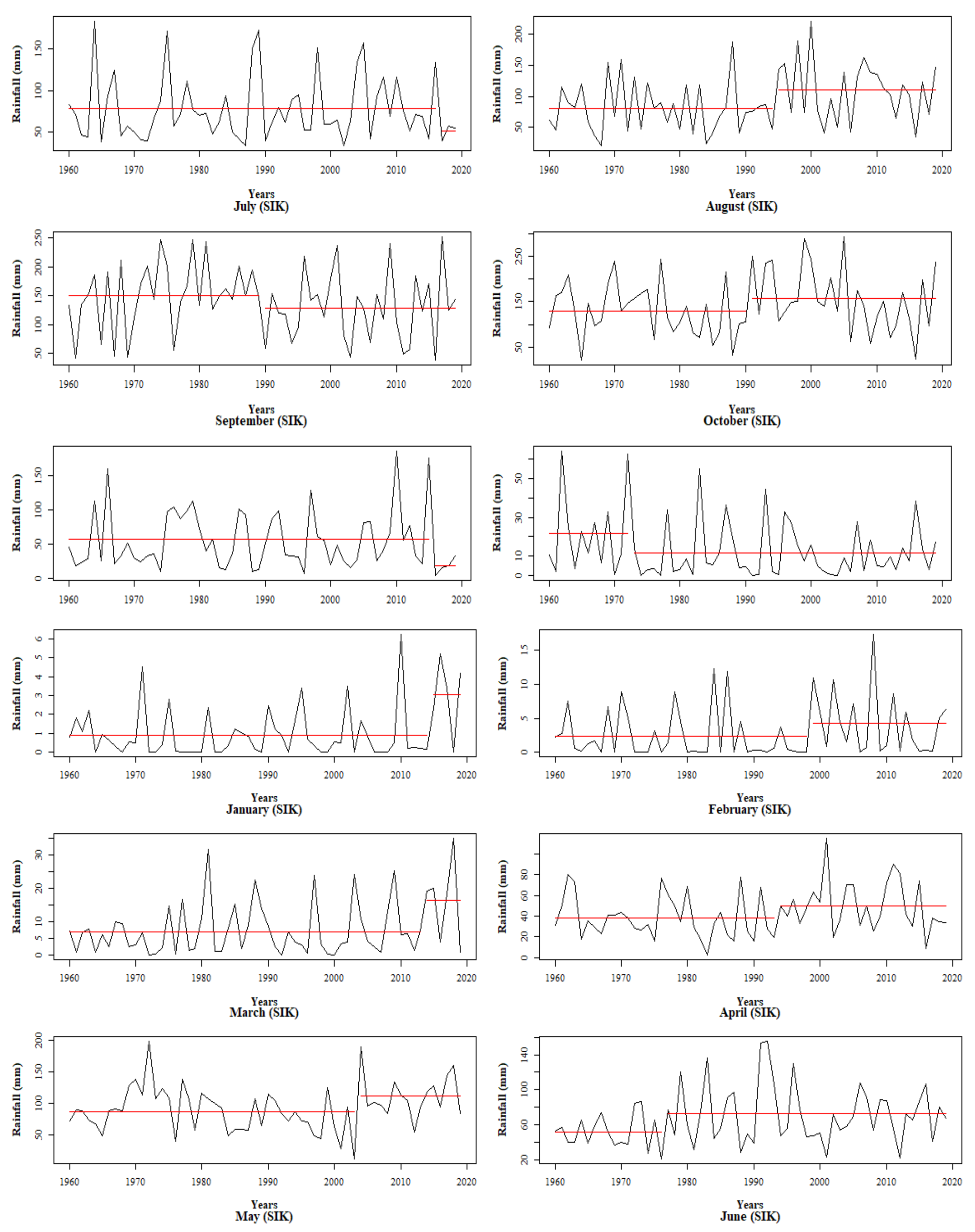
3.2.1. Shifting Pattern in Month-Wise Rainfall Distribution

For each month-wise rainfall data for the period of 60 years from 1960 to 2019 of the SIK subdivision, the shifting point (year) and the average month-wise rainfall (mm) before and after the shifting point (year) were computed and are illustrated in

Table 5. Shifting pattern of monthly rainfall (mm) over SIK.

Month	Shifting Year	Average RF (mm)		Change in RF (mm)	Shifting Nature #	Normal RF (mm)
		Before	After
January	2014	0.9	3.0	2.2	↑	1.8
February	1998	2.3	4.2	2.0	↑	3.5
March	2013	7.1	16.3	9.2	↑	5
April	1993	35.0	50.2	12.1	↑	41
May	2003	56.9	112.8	25.9	↑	96
June	1976	51.5	72.5	21.1	↑	64
July	2016	78.5	50.5	−27.9	↓	79
August	1994	80.0	109.6	29.6	↑	81
September	1989	151.0	128.9	−22.1	↓	135
October	1990	128.5	156.5	28.0	↑	146
November	2015	57.0	15.3	−38.7	↓	50
December	1972	21.5	11.4	−10.1	↓	14

‘#’ indicates ‘No trend’, ‘↑’ indicates increase in trend, ‘↓’ indicates decrease in trend.

along with the nature of shifting and normal rainfall (mm) of each month. The line graph of month-wise rainfall distribution along with rainfall shifting year and the average month-wise rainfall before and after shifting year are shown in Figure 3.

The shifting point (year) in month-wise rainfall was found in all the months for the SIK subdivision, i.e., January (2014), February (1998), March (2013), April (1993), May (2003), June (1976), July (2016), August (1994), September (1989), October (1990), November (2015) and December (1972). The average rainfall in the region was increased (Table 5) in the month of January (2.16), February (1.95), March (9.20), April (12.12), May (25.90), June (21.05), August (29.61) and October (27.97), whereas the average rainfall was decreased in the month of July (−27.93), September (−22.09), November (−38.72) and December (−10.11) as compared with before and after the shifting point in rainfall. Further, it can also be observed that the average rainfall in the month of January, February, March, April, May, June, July, August and October were below the normal rainfall before the shifting year, but it was increased after the shifting year, which was above the normal rainfall except for the month of July. Conversely, in the month of September, November, and December, the average rainfall was above normal rainfall before shifting year, but it was decreased after shifting year, which was below the normal rainfall.

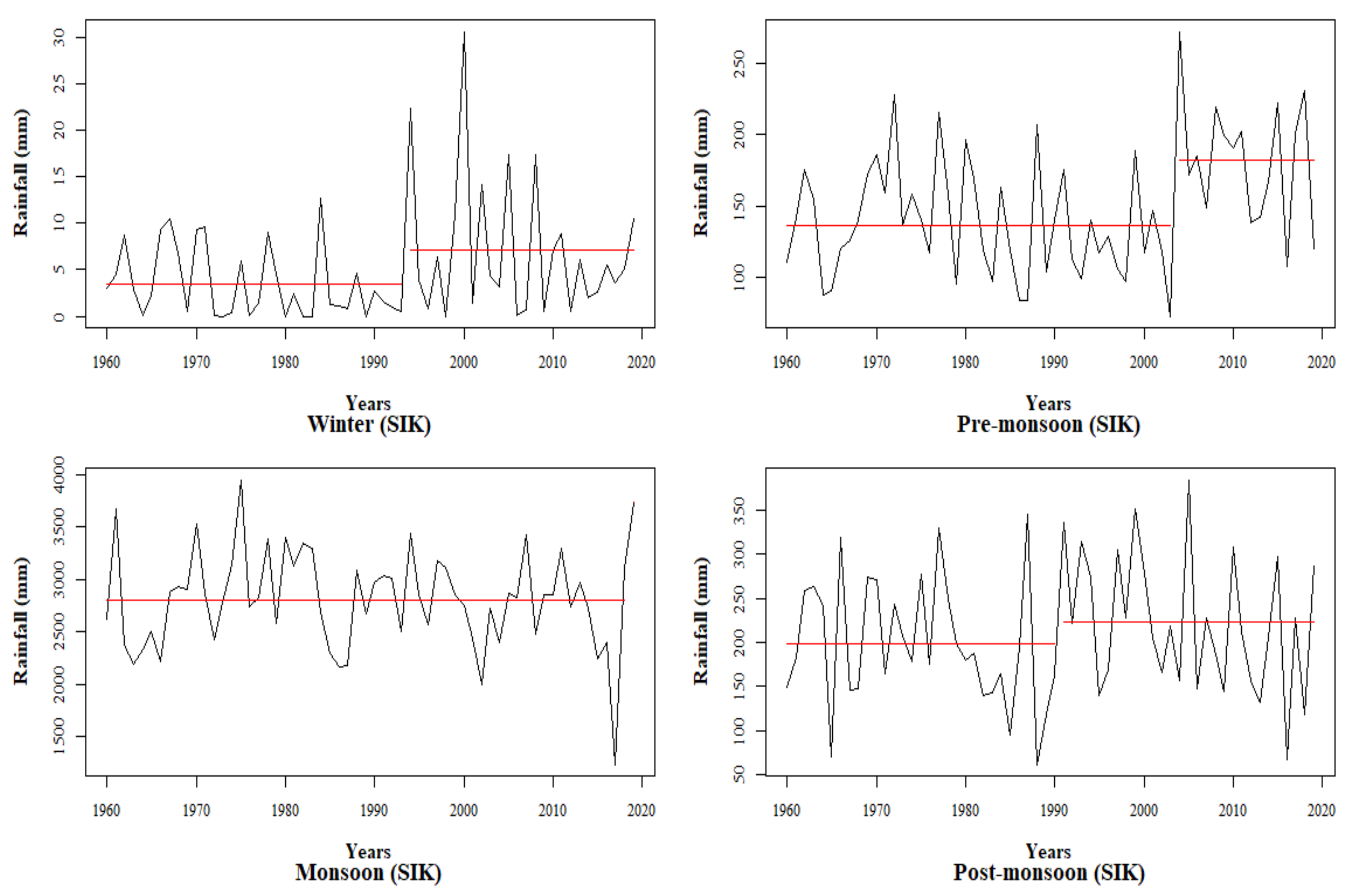
3.2.2. Shifting Pattern in Seasonal Rainfall Distribution

The shifting point (year) in seasonal rainfall was observed in all seasons viz., winter (1993), pre-monsoon (2003), monsoon (1970) and post-monsoon (1990). Results revealed that the average rainfall was increased for winter (3.69), pre-monsoon (45.71), monsoon (65.13) and post-monsoon (24.90) seasons as compared with before and after shifting point in rainfall (

Table 6. The shifting pattern of seasonal rainfall (mm) data of SIK.

Season	Shifting Year	Average RF (mm)		Change in RF (mm)	Shifting Nature #	Normal RF (mm)
		Before	After
Winter	1993	3.5	7.1	3.7	↑	5.0
Pre-monsoon	2003	136.5	182.2	45.7	↑	145.0
Monsoon	1970	322.7	387.9	65.1	↑	359.0
Post-monsoon	1990	198.0	222.9	24.9	↑	210.0
Annual	1968	662.0	753.2	91.2	↑	719.00

‘#’ indicates ‘No trend’, ‘↑’ indicates increase in trend.

). Further, the average seasonal rainfall in winter, pre-monsoon, monsoon and post-monsoon was below normal rainfall before shifting year, but it was increased after shifting year, which was above the normal rainfall (Figure 4).

3.2.3. Shifting Pattern in Annual Rainfall Distribution

As compared with before and after the shifting point in rainfall, the average annual increased for SIK (91.21 mm). Further, the average annual rainfall in the SIK subdivision was below normal rainfall before the shifting year and increased after the shifting year, which was above the normal rainfall. Inter-annual variability is a better (than mean value) and one of the most important indicators of the reliability of rainfall [53,54].

Thus, understanding the regional level of rainfall trends from past data is of importance for agriculture. In the rainfed condition, success or failure of crops is closely linked with rainfall patterns. Therefore, assessing rainfall variability has been an integral part of water resources planning and management [55]. Since there is a direct relationship between rainfall and agriculture, any small amount of change in the distribution pattern of rainfall would adversely affect the production and productivity of crops [56]. Hence, the study of change in the amount, the pattern of rainfall, and its influence on agriculture have become the most important concern for decision making on crop sowing and further activity.

In the dry lands of SIK, two different sowing strategies are used by the farmers: ‘dry seeding’ and ‘wet seeding.’ The first strategy consists of sowing before the rains, i.e., when the soil is still dry [57]. This practice tends to ease germination, reduces the time needed to prepare farmable land before the first rains. However, this strategy is risky since high soil temperatures associated with dry weather as well as scarce and erratic rainfall before the full installation of the monsoon, which is insufficient for full germination of the plant, may spoil the seeds [58]. As the temporal rainfall variability increased, this strategy is less used [59]. Most farmers now wait for a significant rainy event, usually check the rainfall amount by testing the soil moisture to a certain depth, and then sow the same day or the day after. In most parts of the region, the majority of lands are sown in 5 consecutive days after June’s first fortnight [60]. However, this practice does not eliminate the risk of sowing failure in case of a dry spell just after the sowing because of false onset of monsoon (a dry spell of ≥5 days in the 12 days following the potential start [61,62]. In order to overcome the lacunae of sowing by these farmers’ strategies, novel approaches were developed, one among them is the agro-climatic onset of monsoon proposed by Walter (1967) [31] and further developed by Sivakumar (1988) [23].

The agro-climatic approach defines the onset as the optimal date that ensures sufficient soil moisture during planting and early growing periods to avoid crop failure after sowing [23,29,31,32]. The date of onset of rains in this study is defined as that date after 1 May when rainfall accumulated over 3 consecutive days is at least 20 mm and when no dry spell within the next 30 days exceeds 7 days. This criterion is based on the observations on the establishment of various crops (pigeonpea, finger millet, groundnut, etc.) in the region. Further, the first occurrence of a long dry spell after a specified date could be used as the definition for the end of rain [63]. The date of the end of rain is taken as that date after 1 September, following which no rain occurs over a period of 20 days; this aspect will be worked out in our future studies. The developed MatLab interface requires different inputs for simulating the agro-climatic onset, as explained in

Table 7. Inputs required, fixed values and rationale behind the consideration of values for estimation of Agro-climatic onset.

Input.	Value Fixed	Rationale for Consideration
Start date	April 1	To take into account of pre monsoon showers in the region.
Rainfall threshold (mm)	20 mm	Sufficient for sowing of major dryland crops such as finger millet, pigeonpea and other crops [64].
Dry day threshold (mm)	2.5 mm	Minimum amount of soil moisture to meet the daily evaporation need of soil in study area (red sandy loams).
Dry spell threshold (days)	10 days	Maximum number of days that crop can sustain even after reaching the dry day threshold.
Dry spell search period (days)	20 days	Majority of dryland crops have ability to sustain up to 20 days with minor amounts of soil moisture.

.

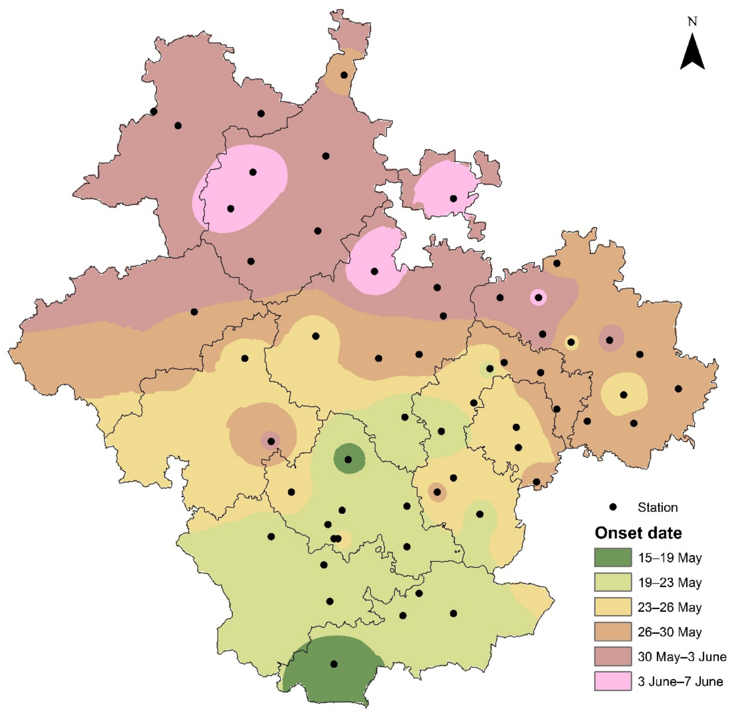
3.2.4. Agro-Climatic Onset of Cropping Season in SIK

For estimating the onset of the cropping season in the study zone, the SIK is divided into three dry farming regions (Table 1), viz., central dry zone (CDZ), eastern dry zone (EDZ) and southern dry zone (SDZ). Zone wise onset of monsoon are explained as below.

CDZ

A dry zone receives an average rainfall of 608.8 mm, and most of it is received during April and May as pre-monsoon showers. The simulation was carried out for all the stations coming under each block of four districts of the zone. We got different onset dates for each block since the variability of rainfall amongst them (Table 2). Among all the blocks, an earlier date of 9 May (

Table 8. The agro-climatic onset of monsoon over SIK (zones CDZ, EDZ and SDZ, subdivided into blocks) expressed in terms of days after the start date and actual date.

Block	DASD	ACOD	Block	DASD	ACOD
CDZ
Chitradurga	38	09-May	Harihara	34	04-June
Hosadurga	32	17-May	Jagaluru	32	02-June
Challakere	34	18-June	Madhugiri	35	05-June
Molakalmuru	30	21-May	Pavagadha	36	21-May
Holalkere	37	22-May	Sira	39	24-May
Hiriyur	32	17-May	Chikkanayakanahhalli	25	10-May
Davanagere	33	17-Jun	Kaduru	25	10-May
EDZ
Gubbi	29	14-May	Anekal	28	13-May
Koratagere	29	14-May	Kolar	23	24-May
Devanahalli	30	15-May	Malur	29	30-May
Doddaballapur	28	13-May	Bangarpet	28	13-May
Nelamangala	30	15-May	Shrinivasapura	28	13-May
Hoskote	30	15-May	Mulabagilu	30	15-May
Ramanagara	25	10-May	Chikkaballapur	34	04-June
Magadi	19	20-May	Siddalaghatta	26	10-June
Kanakapura	22	23-May	Chintamani	32	16-June
Chanapattana	29	30-May	Gudibande	36	06-June
Bangalore North	23	08-May	Gouribidanur	33	03-June
Banalore south	23	08-May	Bagepalli	30	14-June
SDZ
Mandya	22	23-May	Nanjanagud	22	23-May
Maddur	20	05-May	Chamarajnagar	19	20-May
Malavally	20	05-May	Yelandur	19	20-May
Shrirangapattana	19	20-May	Gundlupet	15	16-May
Pandavapura	20	05-May	Kollegal	26	11-May
Krishnarajpete	25	26-May	Tumkur	30	15-May
Nagamangala	17	18-May	Kunigal	19	20-May
Mysore	22	23-May	Tiptur	21	22-May
K R Nagar	22	07-May	Channarayapattana	32	17-May
T Narasipura	27	12-May	Arasikere	26	11-May

DASD: days after the start of the simulation, ACOD: the agro-climatic onset date.

) was predicted by the model (38 days after the start of the simulation. That is, 15 April). The average of all the dates simulated for each station indicated that 14 June will be the agro-climatic onset date (30 days after the start of the simulation. That is 15 May).

EDZ

This zone receives an average annual rainfall of 776.7 mm, and 19.2% (149 mm) of total rainfall is received during January–May, 52.1% (404 mm) during June–September and the remaining 28.7% during October–December (223 mm). Due to this temporal and spatial variability of rainfall, different onset dates were simulated by the model for different blocks coming under each district of the zone (Table 2). Among all the blocks, an earlier date of 8th May (23 days after the start of the simulation; 15 April as a start date) was predicted by the model for Bangalore north block (Table 8). In this zone, 13 June (28 days after the start of the simulation; 15 May as a start date) is said to be agro-climatic monsoon onset date after taking average of all the dates simulated for each station.

SDZ

An average annual rainfall of 753.4 mm is received by this zone. Of the 734 mm, 27.4% (201 mm) of the total rainfall is received during January–May, 41% (301 mm) during June–September and the remaining 31.6% (232 mm) during October–December. The variability of simulated agro-climatic onset dates was expected due to the spatio-temporal variability of rainfall across each station of the one. The earliest onset date 5th May (20 days after the start of the simulation; April 15th as the start date) was simulated at Maddur, Malavally and Pandavapura blocks of Mandya (Table 8). The zonal average of 23 May was determined (22 days after the start of the simulation; 1 May as the start date).

The agro-climatic onset was not the same for each zone due to spatial variability of rainfall along with temporal variability. Each station differed with respect to the onset date (Figure 5), indicating the need to educate farmers at block levels for decision making on sowing the crops.

4. Discussion

Analysis of daily rainfall data from 1960 to 2019 (60 years), an increasing trend of annual rainfall was observed over the SIK between 1960 and 2019, as shown in Figure 3 and Figure 4. During the study period, there were about 58% with normal annual rainfall, 21% with excess rainfall and 21% with deficit rainfall. Future projections of climate change using Global and Regional Circulation Climate Models with different IPCC emission scenarios indicate an increase of about 5%–10% in summer monsoon rainfall over India [65]. It is also projected that the number of rainy days may decrease by 20%–30%, which would mean that the intensity of rainfall is expected to increase. Extreme rainfall may also increase by the end of the year 2100. Another study shows a significant increasing trend in extreme rainfall events over central India during the last 50 years [66].

Several studies over the region reported that the Indian summer monsoon showed remarkable stability in spite of some decadal variations as well as large inter-annual variability. The long-term series of Indian Summer Monsoon Rainfall (ISMR) has no discernible trends, but decadal departures are found above and below the long-time average alternatively for 3 consecutive decades [67]. There is an increase in the occurrence of extreme rainfall events over northwest India in recent decades. An analysis of the long-term trends in individual monthly mean rainfall over India for the period 1870–2003 from linear fits produces negative slopes (average 0.09 mm/year) for June, July and September and a significant positive slope of similar value for August [15,68,69]. This envisages searching for alternative crop production practices.

The trend and shift in rainfall patterns in southern Karnataka imply early onset and cessation of monsoon. Under such conditions, by considering defining inputs such as rainfall threshold, dry day threshold, dry spell threshold etc., the date of onset is estimated as 15th May in most parts of the SIK. This emphasizes the advancement of sowing dates in the region for reducing crop losses due to early-season droughts. Early sown crop (May) has the benefit of 657 mm of mean rainfall with 38 rainy days and can grow up to 125 days [70]. This can be evidenced by higher yields of crops such as groundnut (2780 kg/ha) with early sowing (25 May) [71]. The yield of pigeonpea crop sown on the second fortnight of May was significantly higher (1149 kg/ha) as compared to June’s first fortnight (901 kg/ha) [72]. Therefore, sowing in this period can be considered as optimum for higher crop productivity. Any normal rainfed crops such as pulses, finger millet, paddy tanked or direct sown paddy and groundnut can be comfortably grown during this period. In the late sowing period, due to delayed rains, medium-duration crops (finger millet, sunflower, pulses) can be sown with the adoption of efficient intercrops. In the very late rainfall situation, only short-duration crops have to be preferred (cowpea, green gram, horse gram, field bean, vegetables) either for subsistence or for fodder purposes [73].

Further, there is a need for subjective tuning (namely amount of rainfall and length of the initial wet spell, length and intensity of post-onset dry spell, etc.) since the onset date is equivocal [41]. In the future, efforts should be made to estimate the cessation dates based on the agro-climatic approach based on other intra-seasonal characteristics of the rainy season, notably the wet or dry spells distribution, especially close to the end of the rainy season. Any medium-term or seasonal prediction of the timing or intensity of the monsoon’s withdrawal would thus have a critical impact on crop productivity too because of scarcity or abundance during maturity and harvest period [70,74].

5. Conclusions

The first rainy event with at least 20 mm of rainfall a generally been the stratagem to take up sowing of a monsoon crop in SIK. However, the germinating seedlings have to experience severe to lethal levels of moisture stress if the subsequent rainfall episodes are not sufficiently intense, often referred to as false onset of monsoon, which usually occurs later than the first wet spell [34]. A dry spell of more than seven days during the early stages of the crop growth leads to failure of the crop, necessitating re-sowing. Therefore, it is essential to take into account of rainfall threshold, dry day threshold, dry spell threshold and other edaphic variables in order to arrive at a perfect date of onset of monsoon to decisively plan the most profitable crop sowing schedules that would, in turn, reduce yield losses caused due to early-season drought stress.

References

1. Krishnan, R.; Zhang, C.; Sugi, M. Dynamics of breaks in the Indian summer monsoon. J. Atmos. Sci. 2000, 57, 1354–1372. [Google Scholar] [CrossRef]
2. Mccarthy, J.; Canziani, O.; Leary, N.; Dokken, D.; White, K. Climate Change 2001: Impacts, Adaptation, and Vulnerability. Contribution of Working Group II to the Fourth Assessment Report of the Intergovernmental Panel on Climate Change; Cambridge University Press: Cambridge, UK, 2001; pp. 19–25. [Google Scholar]
3. Khanday, M.Y.; Javed, A. Impact of climate change on land use/land cover using remote sensing and GIS in Chopal watershed, Guna, Madhya Pradesh (India). J. Envnt. Res. Dev. 2008, 2, 568–579. [Google Scholar]
4. IPCC. Summary for policymakers. In Climate Change 2007: The Physical Sciences Basis; Cambridge University Press: Cambridge, UK, 2007. [Google Scholar]
5. Subash, N.; Sikka, A.K.; Ram Mohan, H.S. An investigation into observational characteristics of rainfall and temperature in central northeast India: A historical perspective 1889–2008. Theor. Appl. Climatol. 2011, 103, 305–319. [Google Scholar] [CrossRef]
6. Vijaya Kumar, P.; Bal, S.K.; Subba Rao, A.V.M. All India Coordinated Project on Agrometeorology, Annual Report (2018–19); ICAR Central Research Institute for Dryland Agriculture: Hyderabad, India, 2019; pp. 1–144. [Google Scholar]
7. Delitala, A.; Cesari, D.; Chesa, P.; Ward, M. Precipitation over Sardinia (Italy) during the 1946–1993 rainy season and associated large scale climate variation. Int. J. Climatol. 2000, 20, 519–541. [Google Scholar] [CrossRef]
8. Indian Meteorological Department (IMD). 2015. Available online: http://www.imd.gov.in (accessed on 26 November 2020).
9. Prasad, V.S. Onset and withdrawal of Indian summer monsoon. Geophys. Res. Let. 2005, 32, L20715. [Google Scholar] [CrossRef]
10. Goswami, B.N.; Wu, G.; Yasunari, T. The annual cycle, intra seasonal oscillations, and roadblock to seasonal predictability of the Asian summer monsoon. J. Clim. 2006, 19, 5078–5099. [Google Scholar] [CrossRef]
11. Taniguchi, K.; Koike, T. Comparison of definitions of Indian summer monsoon onset: Better representation of rapid transitions of atmospheric conditions. Geophys. Res. Let. 2006, 33, L02709. [Google Scholar] [CrossRef]
12. Fasullo, J.; Webster, P.J. A hydrological definition of Indian Monsoon onset and withdrawal. J. Clim. 2003, 16, 3200–3211. [Google Scholar] [CrossRef] [Green Version]
13. Rajagopalan, B.; Molnar, P. Combining regional moist static energy and ENSO for forecasting of early and late season Indian monsoon rainfall and its extremes. Geophys. Res. Let. 2014, 41, 4323–4331. [Google Scholar] [CrossRef]
14. Wang, B.; Ding, Q.; Joseph, P.V. Objective definition of the Indian summer monsoon onset. J. Clim. 2009, 22, 3303–3316. [Google Scholar] [CrossRef] [Green Version]
15. Stolbova, V.; Surovyatkina, E.; Bookhagen, B.; Kurths, J. Tipping elements of the Indian monsoon: Prediction of onset and withdrawal. Geophys. Res. Let. 2016, 28, 3982–3990. [Google Scholar] [CrossRef] [Green Version]
16. Flatau, M.K.; Flatau, P.J.; Rudnick, D. The dynamics of double monsoon onsets. J. Clim. 2001, 14, 4130–4146. [Google Scholar] [CrossRef]
17. Dore, M.H.I. Climate change and changes in global precipitation patterns: What do we know? Environ. Int. 2005, 31, 1167–1181. [Google Scholar] [CrossRef]
18. Bhowmik, M.; Das, N.; Ahmed, I.; Debnath, J. Rainfall frequency analysis to predict flood in west Tripura district, Tripura, north-east India. Int. J. Geomat. Geosci. 2017, 7, 310–320. [Google Scholar]
19. Karim, T.H.; Keya, D.R.; Amin, Z.A. Temporal and spatial variations in annual rainfall distribution in Erbil province. Outlook Agric. 2018, 47, 59–67. [Google Scholar] [CrossRef]
20. Husak, G.J.; Michaelsen, J.; Funk, C. Use of the gamma distribution to represent monthly rainfall in Africa for drought monitoring applications. Int. J. Climatol. 2007, 27, 935–944. [Google Scholar] [CrossRef]
21. Venkatesh, H.; Shivaramu, H.S.; Rajegowda, M.B.; Rao, V.U.M. Agroclimatic Atlas Karnataka. 2016, p. 211. Available online: https://www.uasbangalore.edu.in/index.php/research-en/agrometerology-en (accessed on 21 January 2021).
22. Pulakeshi, H.B.P.; Patil, P.L.; Dasog, G.S.; Radder, B.M.; Bidari, B.I.; Mansur, C.P. Mapping of nutrients status by geographic information system in Mantagani village under northern transition zone of Karnataka. J. Agric. Sci. 2012, 25, 332–335. [Google Scholar]
23. Sivakumar, M.V. Predicting rainy season potential from the onset of rains in southern Sahelian and Sudanian climatic zones of West Africa. Agric. For. Meteorol. 1988, 42, 295–305. [Google Scholar] [CrossRef] [Green Version]
24. Maracchi, G.; Bacci, L.; Cantini, C.; Haimanot, M.T. Effect of water deficit in vegetative and post-flowering phases on pearl millet grown in controlled environment. Agric. Med. 1993, 123, 65–71. [Google Scholar]
25. Ingram, K.T.; Roncoli, M.C.; Kirshen, P.H. Opportunities and constraints for farmers of west Africa to use seasonal precipitation forecasts with burkina- faso as a case study. Agric. Syst. 2002, 22, 331–349. [Google Scholar] [CrossRef]
26. Barbier, B.; Yacouba, H.; Karambiri, H.; Zorome, M.; Some, B. Human vulnerability to climate variability in the Sahel: Farmers’ adaptation strategies in northern Burkina Faso. J. Environ. Manag. 2009, 43, 790–803. [Google Scholar] [CrossRef] [PubMed]
27. Steward, J.I. Principles and performance of response farming. In Climatic Risk in Crop Production. Models Management for the Semi-Arid Tropics and Sub-Tropics; Ford, W., Muchow, R.C., Bellamy, Z.A., Eds.; CAB International: Wallinford, UK, 1991. [Google Scholar]
28. Sivakumar, M.V. Empirical analysis of dry spells for agricultural applications in West Africa. J. Clim. 1992, 5, 532–539. [Google Scholar] [CrossRef] [Green Version]
29. Omotosho, J.B.; Balogun, A.A.; Ogunjobi, K. Predicting monthly and seasonal rainfall, onset and cessation of the rainy season in West Africa using surface data. Int. J. Climtol. 2000, 20, 865–880. [Google Scholar] [CrossRef]
30. Traore, S.B.; Alhassane, A.; Muller, B.; Kouressy, M.; Somé, L.; Sultan, B.; Oettli, P.; Ambroise, C.; Siéné, L.; Sangaré, S.; et al. Diop, M.; Dingkuhn, M.; Baron, C. Characterizing and modelling the diversity of cropping situations under climatic constraints in West Africa. Atmos. Sci. Lett. 2010, 12, 89–95. [Google Scholar] [CrossRef]
31. Walter, M.W. Length of rainy season in Nigeria. Niger. Geogr. J. 1967, 10, 123–128. [Google Scholar]
32. Omotosho, J.B. Onset of thunderstorms and precipitation over northern Nigeria. Int. J. Climtol. 1990, 10, 849–860. [Google Scholar] [CrossRef]
33. Bacci, L.; Cantini, C.; Pierini, F.; Marachi, G.; Reyniers, F.N. Effects of sowing date and nitrogen fertilization on growth, development and yield of a short day cultivar of millet (Pennisetum glaucum L.). Eur. J. Agron. 1999, 10, 9–21. [Google Scholar] [CrossRef]
34. Sultan, B.; Janicot, S. The West African monsoon dynamics—The “pre-onset” and “onset” of the summer monsoon. J. Clim. 2003, 16, 3407–3427. [Google Scholar] [CrossRef]
35. Birch, H.F. The effect of soil drying on humus decomposition and nitrogen availability. Plant Soil. 1958, 10, 1–31. [Google Scholar] [CrossRef]
36. Sparling, G.P.; Ross, D.J. Microbial contribution to the increased nitrogen mineralization after air-drying of soils. Plant Soil. 1988, 105, 163–167. [Google Scholar] [CrossRef]
37. Badiane, A.N. Le Statut Organique d’un Sol Sableux de la Zone Centre-Nord du Sénégal. Ph.D. Dissertation, Institut National Polytechnique de Lorraine, Lorraine, France, 1993. [Google Scholar]
38. Andrews, D.J. Effects of date of sowing on photosensitive Nigerian sorghums. Exp. Agric. 1973, 9, 337–346. [Google Scholar] [CrossRef]
39. Stoop, W.A.; Pattanayak, C.M.; Matlon, P.J.; Root, W.R. A Strategy to Raise the Productivity of Subsistence Farming Systems in the West African Semi-Arid Tropics. Proceedings Sorghum in the Eighties; ICRISAT: Patancheru, India, 1981; Volume 2, pp. 519–526. [Google Scholar]
40. Vaksmann, M.; Traoré, S.B.; Niangado, O. Le photo-périodisme des sorghos africains. Agric. Dév. 1996, 9, 13–18. [Google Scholar]
41. Agriculture in Karnataka. Economic Survey Report 2018–2019; Directorate of Economic and Statistics: Karnataka, India, 2019; pp. 2–5.
42. Kodandarama, S.R. Forecasting of Rainfall in Meteorological Subdivisions of Karnataka Using Non-Linear Statistical Models. Master’s Thesis, University of Agricultural Sciences, Bagalore, India, 2020; pp. 21–50. [Google Scholar]
43. Sonali, P.; Nagesh Kumar, D. Review of trend detection methods and their application to detect temperature changes in India. J. Hydrol. 2013, 476, 212–222. [Google Scholar] [CrossRef]
44. Yue, S.; Wang, C. The Mann–Kendall test modified by effective sample size to detect trend in serially correlated hydrological series. Water Res. Manag. 2004, 18, 201–218. [Google Scholar] [CrossRef]
45. Mondal, A.; Kundu, S.; Mukhopadhyay, A. Rainfall trend analysis by Mann-Kendall test: A case study of north-eastern part of Cuttack district, Orissa. Int. J. Geol. Earth Environ. Sci. 2012, 2, 70–78. [Google Scholar]
46. Hinkley, D.V. Inference about the change point in a sequence of random variables. Biometrika 1970, 57, 1–17. [Google Scholar] [CrossRef]
47. Chen, J.; Arjun, K.G. Parametric Statistical Change Point Analysis: With Applications to Genetics, Medicine, and Finance; Springer Science & Business Media: Berlin/Heidelberg, Germany, 2011. [Google Scholar]
48. Hawkins, D.M. Testing a sequence of observations for a shift in location. J. Am. Stat. Assoc. 1977, 72, 180–186. [Google Scholar] [CrossRef]
49. Marteau, R.; Benjamin, S.; Vincent, M.; Agali, A.; Christian, B.; Traore, S.B. The onset of the rainy season and farmers’ sowing strategy for pearl millet cultivation in southwest Niger. Agric. For. Meteorol. 2011, 151, 1356–1369. [Google Scholar] [CrossRef] [Green Version]
50. Marteau, R.; Moron, V.; Philippon, N. Spatial coherence of monsoon onset over western and central Sahel (1950–2000). J. Clim. 2009, 22, 1313–1324. [Google Scholar] [CrossRef] [Green Version]
51. Narayanan, P. Trend analysis and forecast of pre-monsoon rainfall over India. Weather 2016, 71, 94–99. [Google Scholar] [CrossRef] [Green Version]
52. Shapiro, S.S.; Wilk, M.B. An analysis of variance test for normality. Biometrika 1965, 52, 591. [Google Scholar] [CrossRef]
53. Semenov, M.A.; Porter, J.R. Climatic variability and the modelling of crop yields. Agric. For. Meteorol. 1995, 73, 3–4. [Google Scholar] [CrossRef]
54. Corte-Real, J.; Qian, B.; Xu, H. Regional climate change in Portugal: Precipitation variability associated with large-scale atmospheric circulation. Int. J. Climatol. 1998, 18, 619–635. [Google Scholar] [CrossRef]
55. Chakraborty, S.; Pandey, R.P.; Chaube, U.C.; Mishra, S.K. Trend and variability analysis of rainfall series at Seonath river basin, Chhattisgarh (India). Int. J. Appl. Sci. Eng. Res. 2013, 2, 425–443. [Google Scholar]
56. Adarsh, S.; Reddy, J.M. Trend analysis of rainfall in four meteorological subdivisions of southern India using nonparametric methods and discrete wavelet transforms. Int. J. Climatol. 2015, 35, 1107–1124. [Google Scholar] [CrossRef]
57. Ruth, K.; Darshini, R.; Tashinae, S. Local adaptation strategies in semi-arid regions: Study of two villages in Karnataka, India. Clim. Dev. 2015, 9, 1–15. [Google Scholar]
58. Ramachandrappa, B.K.; Thimmegowda, M.N.; Krishnamurthy, R.; Srikanth Babu, P.N.; Savitha, M.S.; Srinivasarao, C.H.; Gopinath, K.A.; Ravindra Chary, G. Usefulness and impact of agromet advisory services in eastern dry zone of Karnataka. Indian J. Dryland Agric. Res. Dev. 2018, 33, 32–36. [Google Scholar] [CrossRef]
59. Amrutha, H.R.; Shreedhar, R. Study of rainfall trends and variability for Belgaum district. Int. J. Res. Eng. Technol. 2014, 3, 148–155. [Google Scholar]
60. Rajegowda, M.B.; Muralidhara, K.S.; Murali, N.M.; Kumar, T.N.A. Rainfall shift and its influence on crop sowing period. J. Agrometeorol. 2000, 2, 89–91. [Google Scholar]
61. Davey, E.G.; Mattei, F.; Soloman, S.I. An Evaluation of Climate and Water Resources for the Development of Agriculture in the Sudano-Sahelian Zone of West Africa; WMO Publication: Geneva, Switzerland, 1976; p. 304. [Google Scholar]
62. Iyengar, R.N. Application of principal component analysis to understand variability of rainfall. Proc. Indian Acad. Sci. 1991, 100, 105–126. [Google Scholar]
63. Stern, R.D.; Dennett, M.D.; Garbutt, D.J. The start of the rains in West Africa. J. Climatol. 1981, 1, 59–68. [Google Scholar] [CrossRef]
64. Morris, R.A.; Zandstra, H.G. Land and climate in relation to cropping patterns in rainfed lowland rice. In Proceedings of the International Rice Research Conference, Los Banos, Philippines, 15 February 1975. [Google Scholar]
65. Shukla, P.R.; Sharma, K.K.; Amit, G. NATCOM Emission scenarios and Carbon Emissions projections for India. V&A Workshop Scenar. Future Emiss. 2003, 27, 1–16. [Google Scholar]
66. Goswami, B.N.; Venugopal, V.; Sengupta, D.; Madhusoodanan, M.S.; Xavier, P.K. Increasing trend of extreme rain events over India in a warming environment. Science 2006, 314, 1442–1445. [Google Scholar] [CrossRef] [Green Version]
67. Subash, N.; Singh, S.S.; Priya, N. Variability of rainfall and effective onset and length of the monsoon season over a sub-humid climatic environment. Atmos. Res. 2001, 99, 479–487. [Google Scholar] [CrossRef]
68. Rajeevan, M.; Bhate, J.; Jaswal, A.K. Analysis of variability and trends of extreme rainfall events over India using 104 years of gridded daily rainfall data. Geophys. Res. Let. 2008, 35, 1–6. [Google Scholar]
69. Patra, P.K.; Behera, S.K.; Herman, J.R.; Maksyutov, S.; Akimoto, H.; Yamagata, Y. The Indian summer monsoon rainfall: Interplay of coupled dynamics, radiation and cloud microphysics. Atmos. Chem. Phys. 2005, 5, 2181–2188. [Google Scholar] [CrossRef] [Green Version]
70. Ravindrababu, B.T.; Rajegowda, M.B.; Janardhana gowda, N.A.; Girish, J. Weekly, monthly and seasonal rainfall at Bengaluru in Karnataka. J. Agrometeorol. 2010, 12, 263–265. [Google Scholar]
71. Reddy, V.C.; Babu, B.T.R.; Yogananda, S.B. Growth and flowering behaviour of groundnut varieties in relation to sowing dates during kharif season. Curr. Res. 2000, 29, 163–165. [Google Scholar]
72. Sharanappa, K.; Shivaramu, H.S.; Thimmegowda, M.N.; Yogananda, S.B.; Prakash, S.S.; Murukannappa. Effect of row spacing, varieties and sowing dates on growth and yield of pigeonpea. Int. J. Curr. Microbiol. Appl. Sci. 2018, 7, 1125–1128. [Google Scholar]
73. Rao, C.S.; Gopinath, K.A. Resilient rainfed technologies for drought mitigation and sustainable food security. Mausam 2016, 67, 169–182. [Google Scholar]
74. Sridhara, S.; Gopakkali, P.; Nandini, R. Rainfall probability analysis for crop planning in Shivamogga block of Karnataka. J. Agrometeorol. 2016, 18, 168. [Google Scholar]
Figure 1. Study area and location of rainfall recording stations.
Agronomy 11 01135 g001
Figure 2. Spatial variability of rainfall over the study area (annual rainfall average of 60 years, 1960–2019).
Agronomy 11 01135 g002
Figure 3. Monthly rainfall distribution along with shifting pattern in SIK over the years (the change in the continuity of horizontal red line indicates the year from which shift in rainfall pattern was observed. The next line starting from above the breakage point indicates a positive shift, i.e., increase in rainfall and vice versa).
Agronomy 11 01135 g003
Figure 4. Seasonal rainfall distribution along with shifting pattern in SIK over the years (the change in the continuity of horizontal red line indicates the year from which shift in rainfall pattern was observed. The next line starting from above the breakage point indicates a positive shift, i.e., increase in rainfall and vice versa).
Agronomy 11 01135 g004
Figure 5. The variability of agro-climatic onset of monsoon over the study area.
Agronomy 11 01135 g005