Spatio-Temporal Analysis of Drought Variability in Myanmar Based on the Standardized Precipitation Evapotranspiration Index (SPEI) and Its Impact on Crop Production

Abstract

Drought research is an important aspect of drought disaster mitigation and adaptation. For this purpose, we used the Standardized Precipitation Evapotranspiration Index (SPEI) to investigate the spatial-temporal pattern of drought and its impact on crop production. Using monthly precipitation (Precip) and temperature (Temp) data from 1986–2015 for 39 weather stations, the drought index was obtained for the time scale of 3, 6, and 12 months. The Mann–Kendall test was used to determine trends and rates of change. Precip and Temp anomalies were investigated using the regression analysis and compared with the drought index. The link between drought with large-scale atmospheric circulation anomalies using the Pearson correlation coefficient (R) was explored. Results showed a non-uniform spatial pattern of dryness and wetness which varied across Myanmar agro-ecological zones and under different time scales. Generally, results showed an increasing trend for the SPEI in the three-time scales, signifying a high tendency of decreased drought from 1986–2015. The fluctuations in dryness/wetness might linked to reduction crop production between 1986–1999 and 2005, 2008, 2010, 2013 cropping years. Results show relationship between main crops production and climate (teleconnection) factors. However, the low correlation values (i.e., <0.49) indicate the extent of the relationship within the natural variability. However, readers are urged to interpret this result cautiously as reductions in crop production may also be affected by other factors. We have demonstrated droughts evolution and trends using weather stations, thus providing useful information to aid policymakers in developing spatially relevant climate change adaptation and mitigation management plans for Myanmar.

1. Introduction

The Intergovernmental Panel on Climate Change (IPCC) [1] stipulates that the worsening of global warming effects will lead to more extreme events such as droughts, floods, and heat waves. Evidence shows that some of these extreme events have already occurred in water-limited regions of the world [1].

As a result, drought has gained attention from academia and other stakeholders [2,3,4]. Drought is a natural disaster [2,5,6,7] that results in a negative impact on several sectors of society, such as, water resources [8], agriculture [8], ecosystems [9,10] and socio-economic impacts [9]. There are four types of droughts, namely, meteorological, hydrological, agricultural, and socio-economic droughts (see Mishra, and Singh, [3], Heim [11] and Yihdego et al. [12] for an extensive review). A specialized drought index is used to measure drought, mainly based on climate or environmental variables used as proxies [12]. Many drought indices have now been developed to detect or characterize droughts events and selecting a particular type of drought index would influence the outcome of a study [3,6,11,12]. The most widely used drought indices in the literature are the standardized precipitation index (SPI), Palmer drought severity index (PDSI) [13] and its variants (self-calibrated PDSI) [14,15,16,17,18]. However, by design, the SPI and PDSI possess some inherent limitations that makes their use in investigating, for example, agriculture droughts inappropriate. The SPI is multiscale by design (i.e., adapt to different timescales), however, uses only atmospheric water supply (i.e., precipitation) as a proxy to infer drought and does not account for atmospheric demand (i.e., evaporative demand) [19].

On the contrary, the PDSI is a simplified soil water balance model that incorporates both precipitation and evaporative demand but not a multi-scalar drought index [20]. Thus, making their use to investigate agriculture (i.e., crop yield and production response) due to drought difficult [21]. However, these limitations were addressed by the development of the standardized precipitation evapotranspiration index (SPEI) [22]. The following literature extensively summarizes recent SPEI based studies at a regional scale, temporal scale, types of datasets used and statistical method used [23,24,25,26,27,28,29,30,31,32,33,34,35,36]. Using different drought indices, most of these studies revealed that SPEI is most sensitive to drought conditions due to the evaporative demand component (as demonstrated in potential evapotranspiration (PET)) indicating SPEI importance as a favorable drought index. This further implies that the SPEI is more robust in revealing droughts due to rising temperature in the context of global warming.

Many studies, using different drought indices, have linked climate-driven factors to agricultural outcomes such as yields and production. In particular, agronomic studies uses these drought indices as tool to evaluate the potential effects of climate change on crop production [37]. If drought occurrences last longer then it may severely impact growth of crops and its impact on the global food production cannot be overemphasized [38].

Agriculture vulnerability to drought conditions has been widely studied. Indeed, there is evidence to show that these severe droughts have impacted crop production or yield thus, threatening regional food security in regions with rain-fed agricultural system. We refer readers to the following literature [references therein] developed different framework to investigate the link between drought and crop production at global scale [37,39,40], USA [41], Europe [42], Asian least developed nations [43,44], China [45], India [46], Australia [47], Africa [44,48].

Also, comparing the results of the different studies, one inevitably finds differences in results. It remains unclear if these differences between studies arise from the different periods of study or reflect uncertainty about the datasets used (e.g., in situ, reanalysis or satellite data).

From the literature, the potential influence of climate variability on crop production is mainly sensitive to rainfall and other inter-variable dependence such as temperature and evapotranspiration variabilities [49,50,51]. This is because crop production needs optimal precipitation and tolerable temperature ranges for growth and development [52], and drought variations may potentially reduce crop production and affect the agricultural systems of countries with no climate literacy or weak implementation strategy [50]. This remains an open question that this study tends to explore.

Therefore, this study fills the gap by contributing to the literature and providing insight into drought studies and its relationship with crop production in Myanmar. FAO [50] reports have mentioned Asia economy to be highly vulnerable to climate change. As agriculture sector still remains the largest employer in most Asia economies, and its sensitivity to varying hydro-climatic conditions (particularly in regions with no or weak agricultural irrigation systems) cannot be overlooked.

In this study, we employ the SPEI developed by Vicente-Serrano et al. [22] based on the added value of representing the multi-scale characteristic of SPI and the sensitivity of PDSI to changes in evaporative demand. In addition, we estimate the link between weather and crop production for the three crops with the largest production value in the Myanmar: rice, wheat, and corn.

Myanmar is one of the most vulnerable countries in the region due to her diverse agro-climatic conditions [49]. Past studies showed that Myanmar has experienced both precipitation and temperature changes over the last decade [53,54,55,56]. These changes have had implication on the length of wet season and influenced farmers decision to grow their crops. For example, few studies found high precipitation and temperature variability to impact crop productivity [49,57]. However, the effect of climate change on Myanmar on the crop production is less explored.

We acknowledge that declines in staple crop production are caused by several factors including agricultural management practices, quality of seeds used, technological investments, fluctuation in crop prices, research and development [56], etc. Nonetheless, this study focuses on climate-driven crop production variability in Myanmar′s major crops. The study outcomes may form a scientific basis to help design droughts mitigation and adaptation policies for different stakeholders in agriculture, water resources, and management, among others.

The present study aims at investigating the spatiotemporal variations, frequency of droughts and its possible connections with variations in SST and crop production anomalies using the SPEI at different time scales and seasons. In addition, it examines the difference between the SPEI based on the average of climatic parameters and the average of SPEI of all locations.

The remainder of this paper is organized as follows; provide a brief description of the study area and a summary of the methods and approaches used in Section 2. Section 3 provides the study results and discussion of findings. In Section 4. we provide the summary and conclusions of the study.

2. Materials and Methods

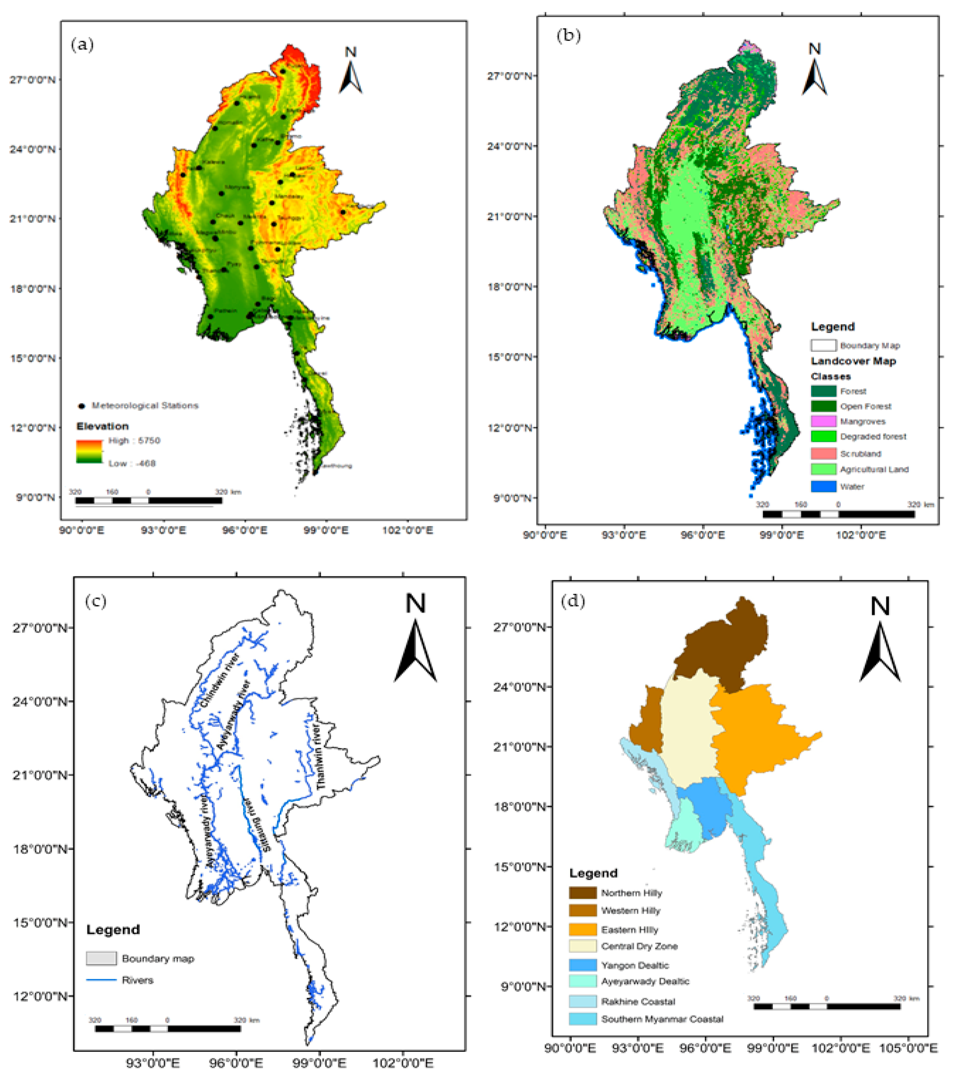
2.1. Study Area

Myanmar is situated in Southeast Asia. A variety of topography such as flat (central), hilly (north, northwest, and east), and coastal (west and south) covers the country. It is bounded by water (Bay of Bengal and the Andaman Sea) in the western part of the country with latitude 9°32′ N–28°31′ N and longitudes 92°10′ E–101°11′ E (Figure 1a–d).

Myanmar is characterized by precipitation a high spatio-temporal variability [53] as a result of its varying topography (Figure 1a) and vegetation cover (Figure 1b). The vegetation cover interacts with the atmosphere in complex ways to affect weather and climate [60]. Based on land use and land cover (LULC) from DIVA-GIS [58], seven dominant classes of LULC were found over Myanmar, namely forest, open forest, degraded land, scrubland, agriculture land, mangroves, and water (Figure 1b).

Myanmar has large rivers that crosses the country (Figure 1c). The figure presents the streamflow of four major rivers across Myanmar. The largest river is the Ayeyarwady (nearly 2170 km in length), which cuts through the country′s fertile lands, followed by the Thanlwin, Sittaung and Chindwin Rivers. Those rivers define Myanmar′s agriculture sector contribution to Gross Domestic Product [50]. This explains the important role of agriculture in the region. More than 65% of the population live in rural areas, and employed under the agricultural sector [51]. The agro-ecological zone map of Myanmar is shown in Figure 1d.

By contrast, temperature variability is low, both spatially and temporally. The highest temperature (34.3 °C) is recorded in April till June, and the lowest (14.4 °C) is recorded in December till February [54].

The precipitation variability and frequent water scarcity unfavorably impact Myanmar′s food security and socio-economic development agenda [61,62]. Moreover, atmospheric circulation drivers have been noted to influence Myanmar′s and its surrounding inter-annual precipitation variability. For example, the El Niño Southern Oscillation (ENSO) and Indian Ocean Dipole (IOD) events are linked to anomalous precipitation in the South East Asia region, leading to extreme floods and droughts, respectively.

2.2. In Situ Observation Data

We used the monthly mean precipitation and monthly mean temperature datasets of 39 meteorological stations spanning from 1986–2015. The data were collected from the Department of Meteorology and Hydrology, Myanmar. The location and specifics of each meteorological station are presented in Figure 1a and

Table A1. List of weather stations with the names and their corresponding geographic locations and elevations.

No.	Station Name	Latitude (°N)	Longitude (°E)	Elevation (m)
1	Bago	17.2	96.3	15
2	Belin	17.13	97.14	61
3	Dawei	14.06	98.13	16
4	Hinthada	17.4	95.25	26
5	Hkamti	26	95.42	146
6	Homalin	24.52	94.55	130
7	Hpa-an	16.45	97.4	9
8	Hsipaw	22.6	97.3	436
9	Kaba-Aye	16.46	96.1	20
10	Kalaywa	23.12	94.18	109
11	Katha	24.1	96.2	113
12	Kawthaung	9.58	98.35	46
13	Kengtung	21.18	99.37	827
14	Kyaukpyu	19.4	93.6	5
15	Lashio	22.56	97.45	747
16	Loikaw	19.41	97.13	895
17	Magway	20.07	94.55	52
18	Mandalay	21.59	96.06	74
19	Mawlamyine	16.3	97.37	21
20	Meiktila	20.5	95.5	214
21	Minbu	20.1	94.53	51
22	Mingladon	16.54	96.11	28
23	Monywa	22.06	95.08	81
24	Myeik	12.26	98.36	36
25	Myitkyina	25.22	97.24	145
26	Naungoo	21.12	94.55	61
27	Pathein	16.46	94.46	9
28	Pinlaung	20.08	96.46	1463
29	Putao	27.2	97.25	409
30	Pyay	18.48	95.13	58
31	Pyinmana	19.43	96.13	101
32	Shwebo	22.35	95.43	106
33	Shwegyin	17.55	96.52	12
34	Sittwe	20.08	92.53	4
35	Taunggyi	20.47	97.03	1436
36	Taungoo	18.55	96.28	47
37	Thandwe	18.28	94.21	9
38	Thaton	16.55	97.22	17
39	Yay	15.15	97.52	3

, respectively. The stations selection was selected based on their long-term temporal coverage, data homogeneity and data record’s completeness. The SST indices such as El Niño-3.4 index derived from the Climatic Prediction Center (CPC)′s, the Extended Reconstructed Sea Surface Temperature version 5 (ERSST v5) data [63]. The Dipole Mode Index (DMI) was derived from the Hadley Centre Global Sea Ice and Sea Surface Temperature (HadISST1.1) [64] were used in this study.

To perform impact of climate change on crop production, the annual crop data series for Myanmar 1986–2015 were downloaded from the Food and Agriculture Organization Statistical Databases (FAOSTAT) website [65] (accessed June 6 2021) to analyze crop production anomalies. For crop production data, we selected three crops for further analysis; namely, corn, wheat and rice. These crops have sufficiently large acreage across Myanmar and uniform distribution over the arable land and thus are comparable during the study period. Figure S2 presents total crop production for the three major crops with their corresponding total hectares grown from 1986–2015.

2.3. Methods

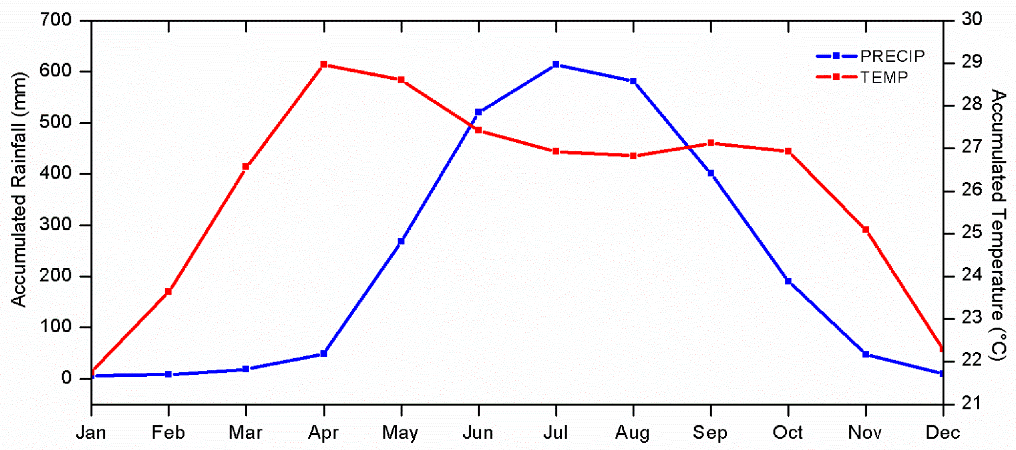
2.3.1. Precipitation and Temperature Climatology

This study calculates monthly accumulated precipitation and temperature from daily data 1986–2015. Seasonal and annual values are then calculated from the monthly data. The display of spatial maps was done in ArcGIS 10.3 (ArcGIS Desktop: Release 10.3) [66].

2.3.2. Calculation of SPEI

To estimate PET, the Penman-Monteith and Thornthwaite models are the two most widely used models. The former provides a better estimate due to its more comprehensive physics [4,14] but it is data intensive and requires more input data that are not usually readily available. The latter is simple as it requires mean monthly temperatures.

The Thornthwaite method (Equation (1); [67] was used as it can capture the main impact of increased temperatures on water demand. The calculation method of Thornthwaite is as follows; Potential evapotranspiration (PET) was calculated using Equation (1).

$$\mathrm{PET}=16K{\left(\frac{10T}{I}\right)}^m$$

(1)

where T is the monthly mean temperature (°C); I is a heat index calculated for the whole year; m is a coefficient depending on $I$, such that m = 6.75 × 10 − 7$I^3$ − 7.71 × 10 − 5 $I^2$ 2 + 1.79 × 10 − 2$I^2$ + 0.492; and K is a correction coefficient defined based on the latitude and month.

The difference between the precipitation (precip) and PET is computed using Equation (2) [22].

$${\mathrm{D}}_{\mathrm{i}}={\mathrm{Precip}}_{\mathrm{i}}-{\mathrm{PET}}_{\mathrm{i}}$$

(2)

D is the difference between the precipitation Precip and PET for the month i and PRECIP is the precipitation. The difference $D_{i,j}^k$ in a given month j of year i depends on the timescale k. For example, the accumulated difference for month i in a particular year i with a 12-month timescale is computed using Equation (3).

$$\begin{gathered} {\mathrm{X}}_{\mathrm{ij}}^{\mathrm{k}}={\displaystyle \sum }_{\mathrm{I}=13-\mathrm{k}+\mathrm{j}}^{12}{\mathrm{D}}_{\mathrm{i}-1,\mathrm{I}}+{\displaystyle \sum }_{\mathrm{I}=1}^{\mathrm{j}}{D}_{i,j}\mathrm{if}\mathrm{j}<{\mathrm{k}\mathrm{and}\mathrm{X}}_{\mathrm{i},\mathrm{j}}^{\mathrm{k}} \\ ={\sum }_{\mathrm{I}=\mathrm{j}-\mathrm{k}+1}^{\mathrm{j}}{\mathrm{D}}_{\mathrm{I},\mathrm{I}}\mathrm{if}\mathrm{j}\ge \mathrm{k} \end{gathered}$$

(3)

where ${\mathrm{D}}_{\mathrm{I},\mathrm{I}}$ (mm) is the PRECIP −PET difference in the first month of the year i. The water balance is normalized based on a log-logistic probability distribution to obtain the SPEI time series. The probability density function of a variable with a log-logistic distribution is expressed as Equation (4):

$$f\left(x\right)=\frac{\beta }{\alpha }{\left(\frac{x-\gamma }{\alpha }\right)}^{\beta -1}{\left[1+\frac{x-\gamma }{\alpha }\right]}^{-2}$$

(4)

where α, β, and γ are the scale, shape, and origin parameters, respectively, for D values in the range $\gamma <D<\infty$. Thus, the probability distribution function of series D f(x) is given by the following Equation (5).

$$f\left(x\right)={\left[1-\frac{\alpha }{x-\gamma }\right]}^{-1}$$

(5)

The SPEI was estimated in an R statistical software [68].

Drought was analyzed with SPEI at 3, 6, 12-month timescales [19].

To better understand the extent and intensity of drought, the drought frequency (F) value was used. The F-value was calculated using the following Equation (6).

$$F_i=\frac{n}{N}\times 100\%$$

(6)

where, n is the number of drought years at the station, N is the total number of years for the precipitation data, and i represents the meteorological station.

2.3.3. Standardized Anomaly Estimation

We estimated the standardized anomaly for precipitation, temperature and the three different crops production in Myanmar based on Equation (A6) in Appendix A.3.

2.3.4. Statistical Analysis

Mann–Kendall test [69] was used to determining trends and rates of change. The formula and estimation procedure are presented in Equations (A1)–(A4) in Appendix A.1. In addition, we used the least square method Equation (A5) to compute the linear trend in precipitation and temperature anomalies. We also performed a correlation analysis Equation (A6); Appendix A.2) to describe the relationship between SPEI and remote drivers (i.e., ENSO and IOD).

In addition, performed a correlation analysis to assess the link between annual SPEI and crop production across multiple years. We also analyzed using seasonal SPEI to investigate its impact on crop production since Myanmar has two crop growing seasons. We selected May-June-July (MJJ), August-September-October (ASO), and MJJASO as seasons to study its effect on crop production.

Statistical analysis was performed using R and Python softwares [68]. Many hydro-meteorological studies have adopted this kind of approach [70,71,72,73].

3. Results

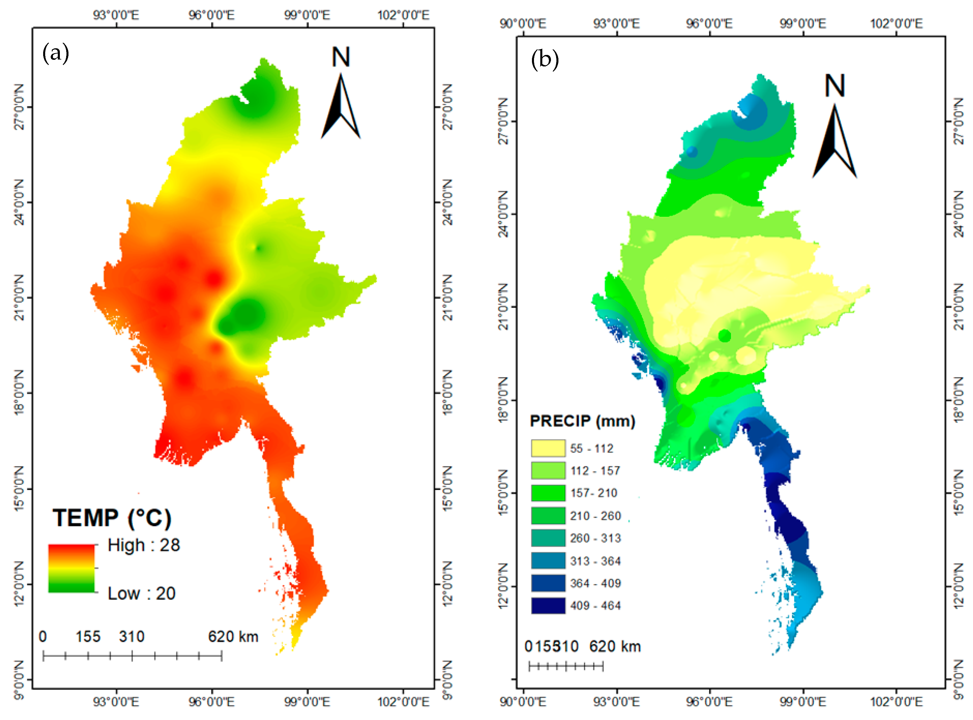
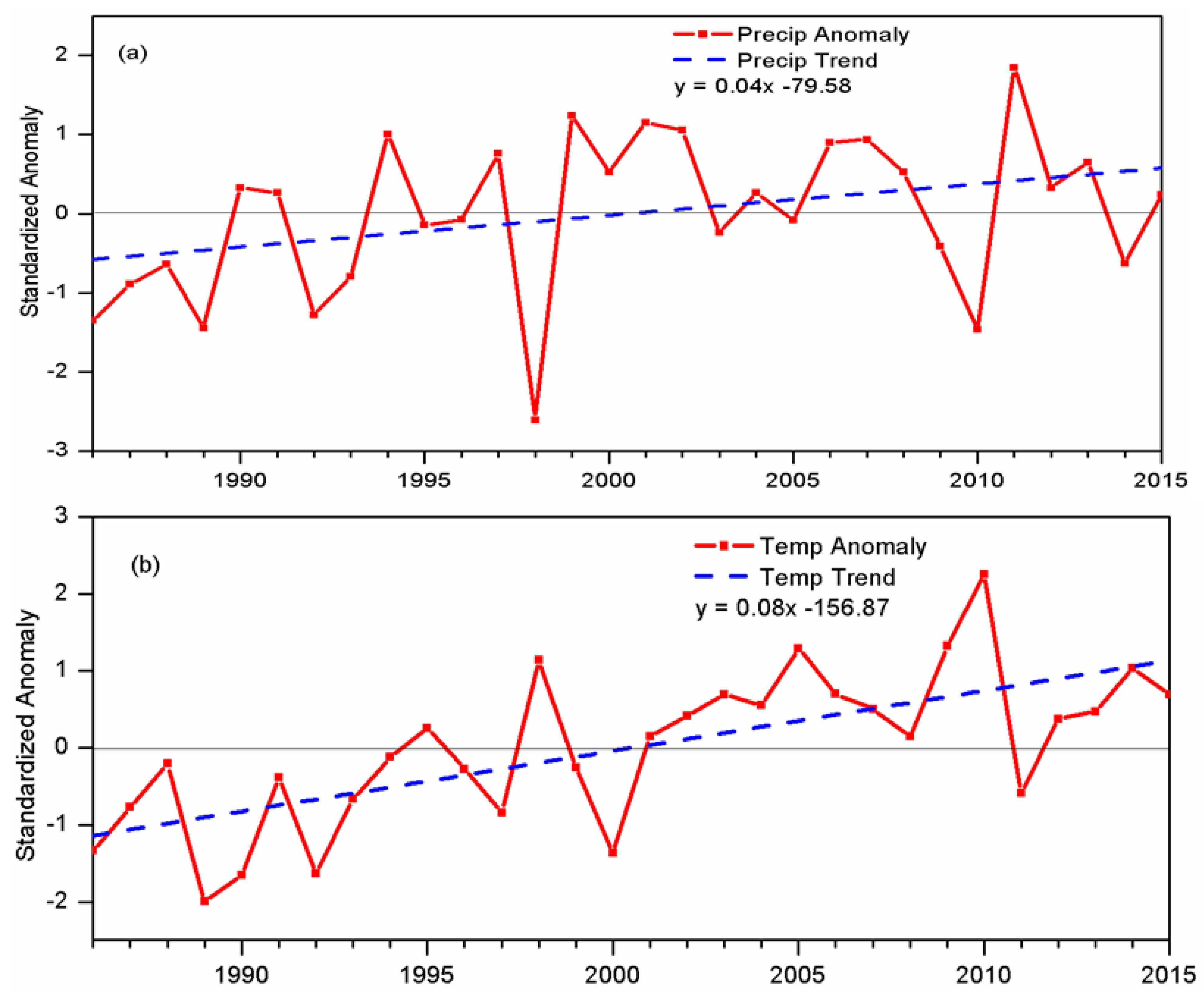
3.1. Climatology and Linear Trend of Temperature and Precipitation

Figure 2 presents the long-term spatial distribution (1986–2015) annual mean of Temp and Precip. Temp has a bi-modal distribution with warmer temperatures on central, Rakhine coastal, Yangon deltaic, Ayeyarwady deltaic and southern Myanmar coastal and cooler temperatures on the north hilly and eastern hilly (Figure 2b). The results of Temp explain the country received the coldest place on north hilly and eastern hilly while hottest place on central, Rakhine coastal, Yangon deltaic, Ayeyarwady deltaic and southern Myanmar coastal (Figure 2b).

The Mean annual Temp of north hilly and eastern hilly shows (20 °C) and central, Rakhine coastal, Yangon deltaic, Ayeyarwady deltaic and southern Myanmar coastal explains (28 °C) (Figure 2b). Spatial distribution of Precip explains lowest Precip (central dry zone to eastern-hilly zones) while highest Precip (Rakhine coastal and southern Myanmar coastal) (Figure 2a). The annual Precip (Figure 2a) ranges from about 55 mm < Precip < 112 mm (central dry zone to eastern-hilly zones) and ranges from about 409 mm < Precip < 464 mm (Rakhine coastal and southern Myanmar coastal).

On the other hand, Precip and Temp follows the topography. The hilly region received less Temp and coastal and central dry zone received high Temp. The Rakhine coastal and southern Myanmar coastal received highest Precip due to the modulated by summer monsoon season over Southeast Asia.

Also, the PET results indicate that the effect of PET is an important hydro-climatic variable in the Myanmar (Figure S1). The PET values are linked with the Precip and Temp distribution in the region. The spatial pattern of PET (Figure S1a) results shows the north hilly and eastern hilly receive low PET values. However, central, Rakhine coastal, Yangon deltaic, Ayeyarwady deltaic and southern Myanmar coastal show high PET. Figure 3 shows the annual variation in Temp and Precip over Myanmar from 1986–2015. We observed that the Temp pattern is bi-modal, with the highest peak in April (summer season) and the second in October (late monsoon period). Moreover, a unimodal precipitation pattern corresponding to the summer monsoon season from May-October is observed. The highest Precip peak is found in June-July-August. Overall, we found a distinctive characteristic in spatial Temp and Precip patterns (Figure 3). When the Precip is high as oppose Temp is low in the region. It is modulated by Indian monsoon season over Myanmar. In addition, the estimated values in temporal PET patterns (Figure S1b) are largely associated with the Precip, Temp and other hydro-climate and teleconnections variabilities in the region.

In addition, we plotted the inter-annual variation in precipitation and temperature standardized anomalies from 1986 to 2015 (Figure 4). The result showed both temperature and precipitation exhibited an increasing trend.

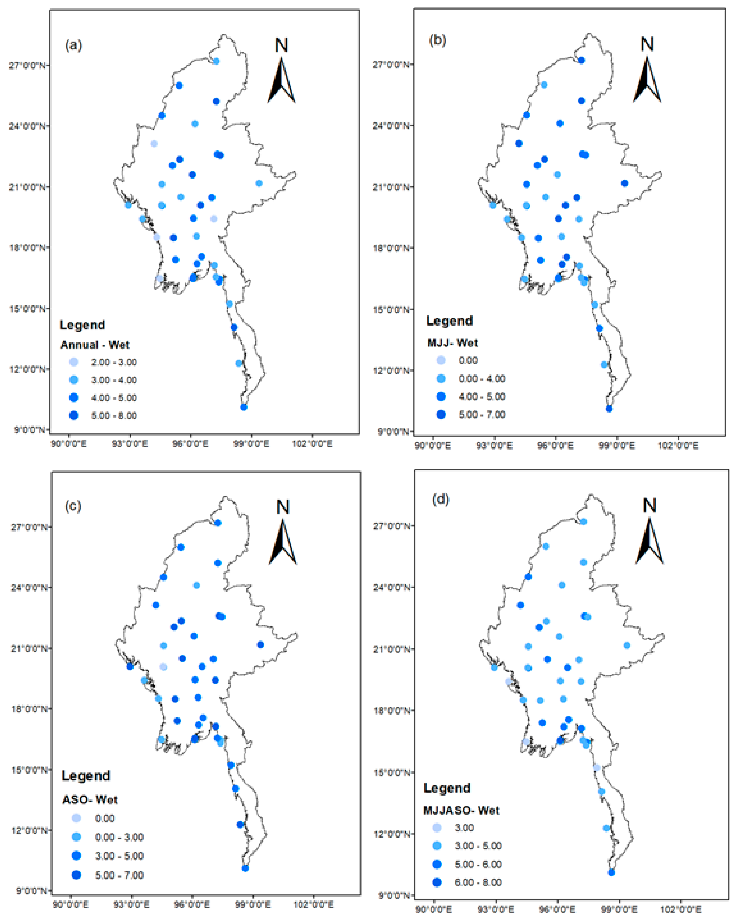
3.2. Spatial–Temporal Trends of Wetting and Drying

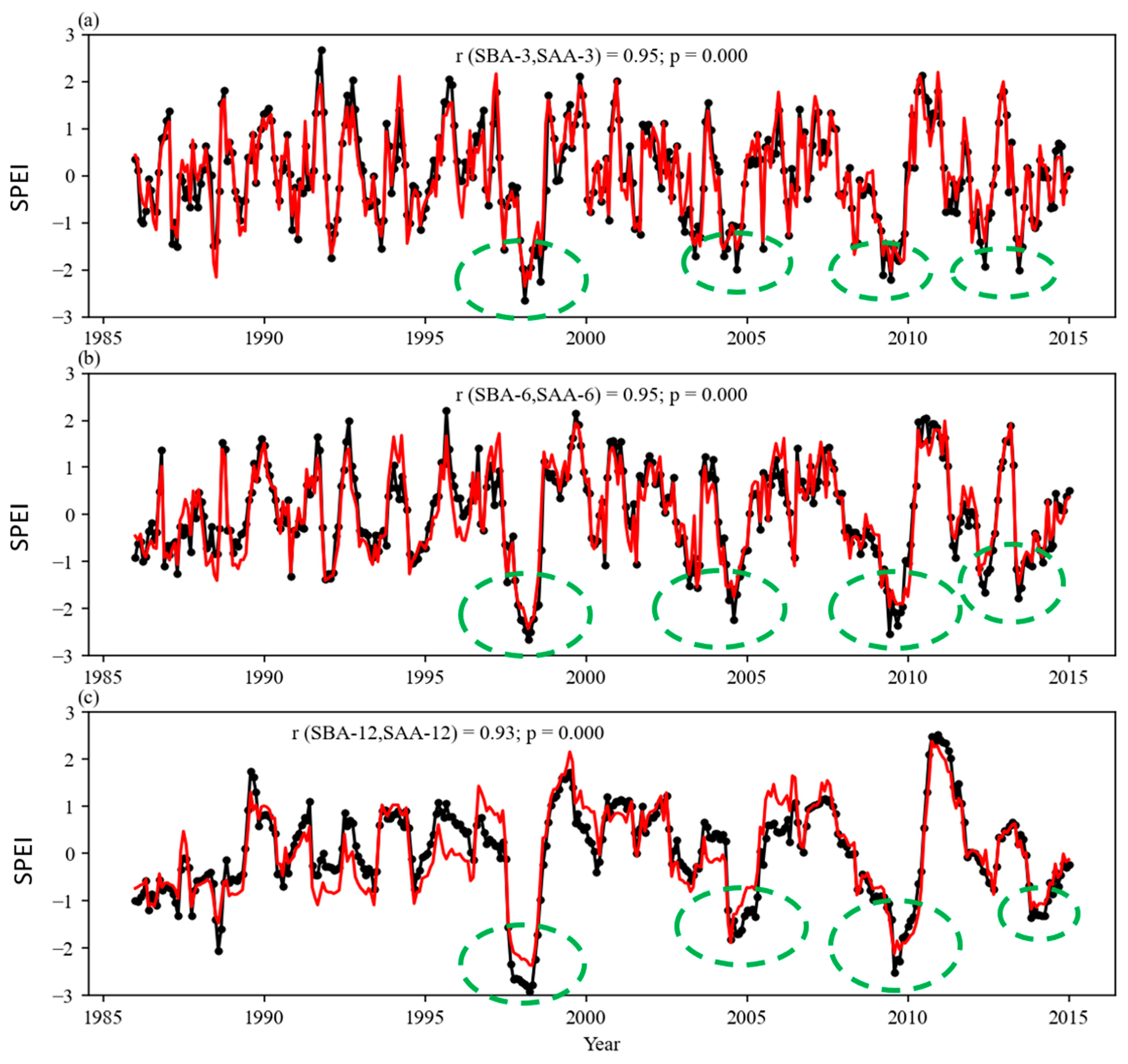
3.2.1. Temporal Variations in Wetting and Drying Trends

Figure 5 describes the area average of SPEI (SAA) and SPEI based on area average of climatic parameters (SBA) over the period of study (1986–2015). The SAA was obtained by averaging SPEI of each location, while SBA is directly obtained after averaging the monthly precipitation and temperature before calculating the SPEI over Myanmar. The SAA was standardized to unit before calculating its interdependence with SBA. Significant and positive correlation coefficients are obtained between SAA and SBA for the three-time scales, i.e., 3-, 6- and 12-months. This means that area average of climate variables is useful to characterize the drought condition over Myanmar, which is in line with Barren et al., [74].

Overall, the temporal patterns for SPEI-3, SPEI-6 and SPEI-12, and the patterns for years with dryness and wetness are similar however differences in their relative magnitudes can be noted. It is found that short-term climate conditions (SPEI-3 and SPEI-6) in Figure 5a,b are closer to each other than that of long-term climatic conditions (SPEI-12).

From Figure 5a, it is observed that the SPEI-3 and SPEI-6 and SPEI-12 showed 1998 as the extreme drought year. Meanwhile, the magnitude of drought intensity are higher as the time scale increases.

Table 1. Classification of SPEI over Myanmar during 1986–2015.

Classes	Category	SPEI-3 (%)	SPEI-6 (%)	SPEI-12 (%)
$\ge 2$	Extremely wet	1.4	0	1.72
1.5 to 1.99	Very wet	4.47	5.91	3.44
1.00 to 1.49	Moderately wet	11.73	13.24	11.46
0.00 to 0.99	Mildly wet	31.84	29.86	30.94
0.00 to −0.99	Mild drought	32.12	34.93	38.97
−1.00 to −1.49	Moderate drought	11.73	10.14	7.16
−1.5 to −1.99	Severe drought	4.75	4.79	3.15
$\le -2$	Extremely drought	1.4	1.13	3.15

shows the classification of SPEI′s (in terms of intensities) over Myanmar from 1986 to 2015. The SPEI-3 showed the highest occurrence of droughts, followed by SPEI-6. SPEI-12 showed the lowest percentage of extreme droughts. Between 1986 and 2015, it is found that SPEI-3 show dominant severe droughts over very wet conditions. Meanwhile, the SPEI-6 show a dominant very wet conditions over severe droughts.

Concerning the SPEI-12, a high occurrence of extreme drought is observed, while a low occurrence of extreme wet condition is evident.

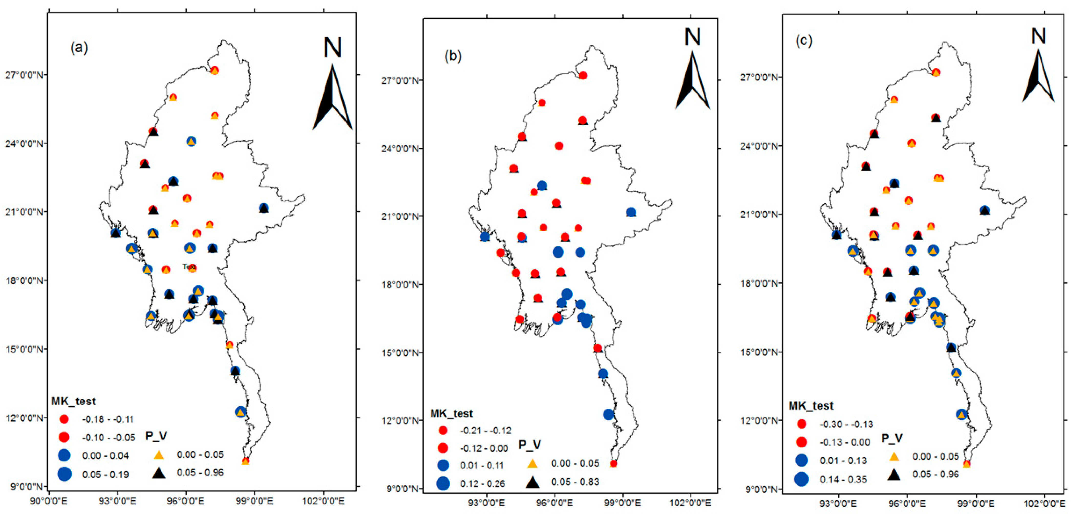
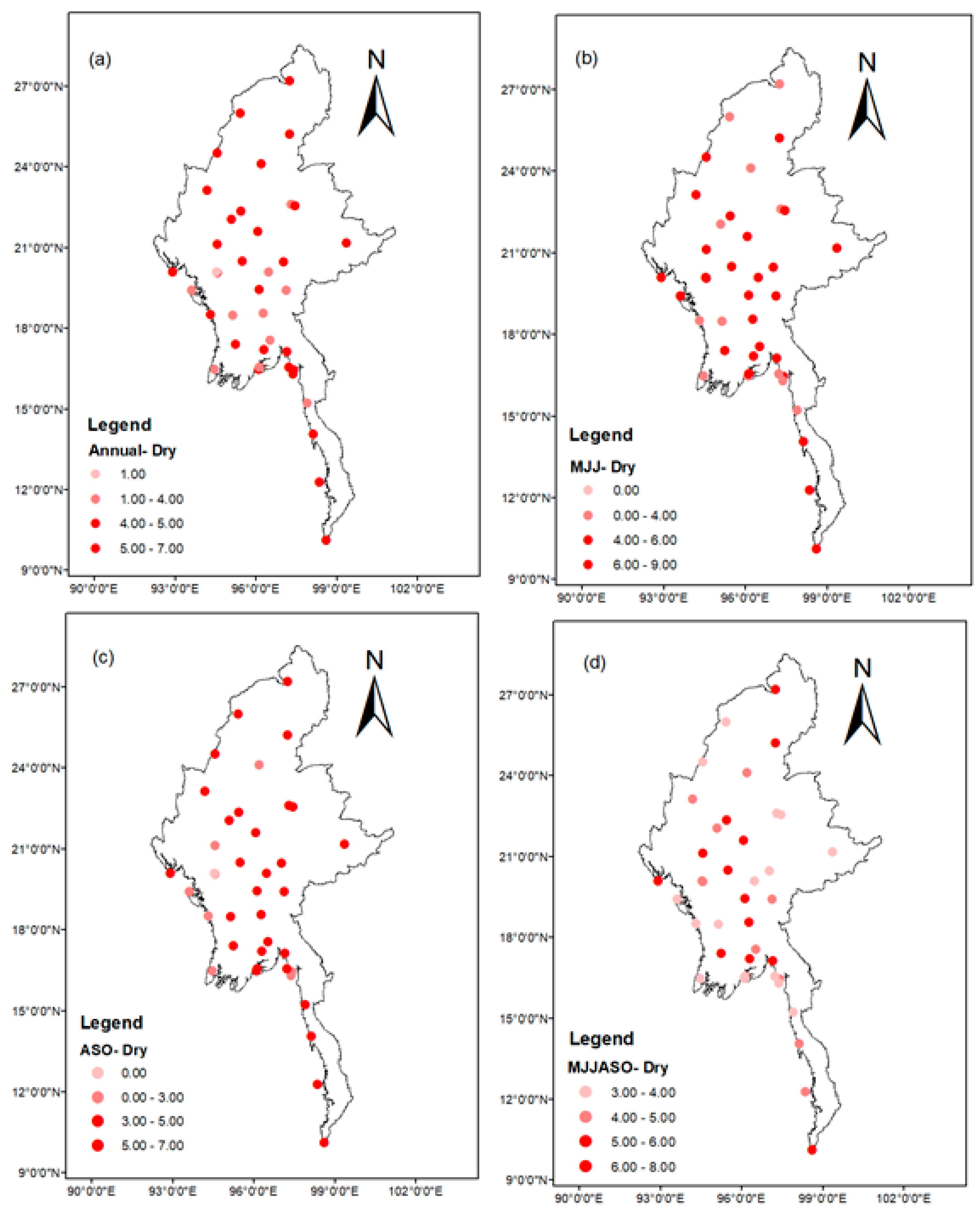
3.2.2. Spatial Variations in Wetting and Drying Trends

The monotic trend analysis of SPEI at 3, 6, 12-months was examined using the Mann–Kendall test at 5% significance level [69]. Figure 6 shows the precipitation trends from 1986 to 2015. These results help us understand the spatial distributions of individual station linear trends for different SPEI during the study period.

Results of SPEI-3 show increasing trends mainly in the western hilly, deltaic (along the coastal region), and central and east parts (Figure 6a). We observed that few stations located in the central dry area show increasing and decreasing trends. On the contrary, stations located in the northern hilly zone show a decreasing trend (Figure 6a).

The spatial pattern of the SPEI-6 shows increasing trends at many stations in the deltaic zone (but not significant at both 5 and 10%, except for few stations). We observe larger increasing trends in the southern-most portion of the deltaic zone.

Notably, in the central hilly and western hilly, many stations showed a mixed spatial pattern of increasing and decreasing trends. The SPEI-6 results for the northern hilly area are similar to SPEI-3, with the stations showing decreasing trends. SPEI-12 denotes long-term droughts (Figure 6c). The SPEI-12 results are similar to SPEI-6 but with statistically significant results across Myanmar. Moreover, the highest increasing trends are shown for long-term droughts.

We quantitively evaluated the spatial variability of drought frequency across Myanmar in the different SPEI by computing the SPEI frequency distribution for the annual and seasonal basis to understand the regional wetting and drying conditions. We obtained the drought frequency at each station and based on a spatial analysis method, interpolated the results to obtain different drought frequencies at a country-level. Figure 7 and Figure 8 presents the spatial distribution of drought frequency for the three different levels of drought for 1986–2015.

We observed that the western hilly areas and patches in the deltaic eco-zones along the coastal region showed the highest frequency of dry spells as compared with wet spells in the same period. The findings showed similar spatial distributions for different seasons but with varying values (Table 1).

Taking MJJ as an example, fewer dry spells than wet spells persisted with varying frequencies (Figure 7b and Figure 8b). In ASO, the frequency of dry spells is found in nearly the entire country, with deltaic, western, and eastern hilly zones showing a more pronounced frequency of dry spells. In contrast, wet spells in ASO (Figure 8c) showed similar spatial patterns to Figure 7c (MJJ wet spells), but with significant frequency values. In the monsoon season, the frequency of dry spells was high (4–7 times) in most areas from deltaic, western, and eastern hilly zones compared with wet spells in both space and time.

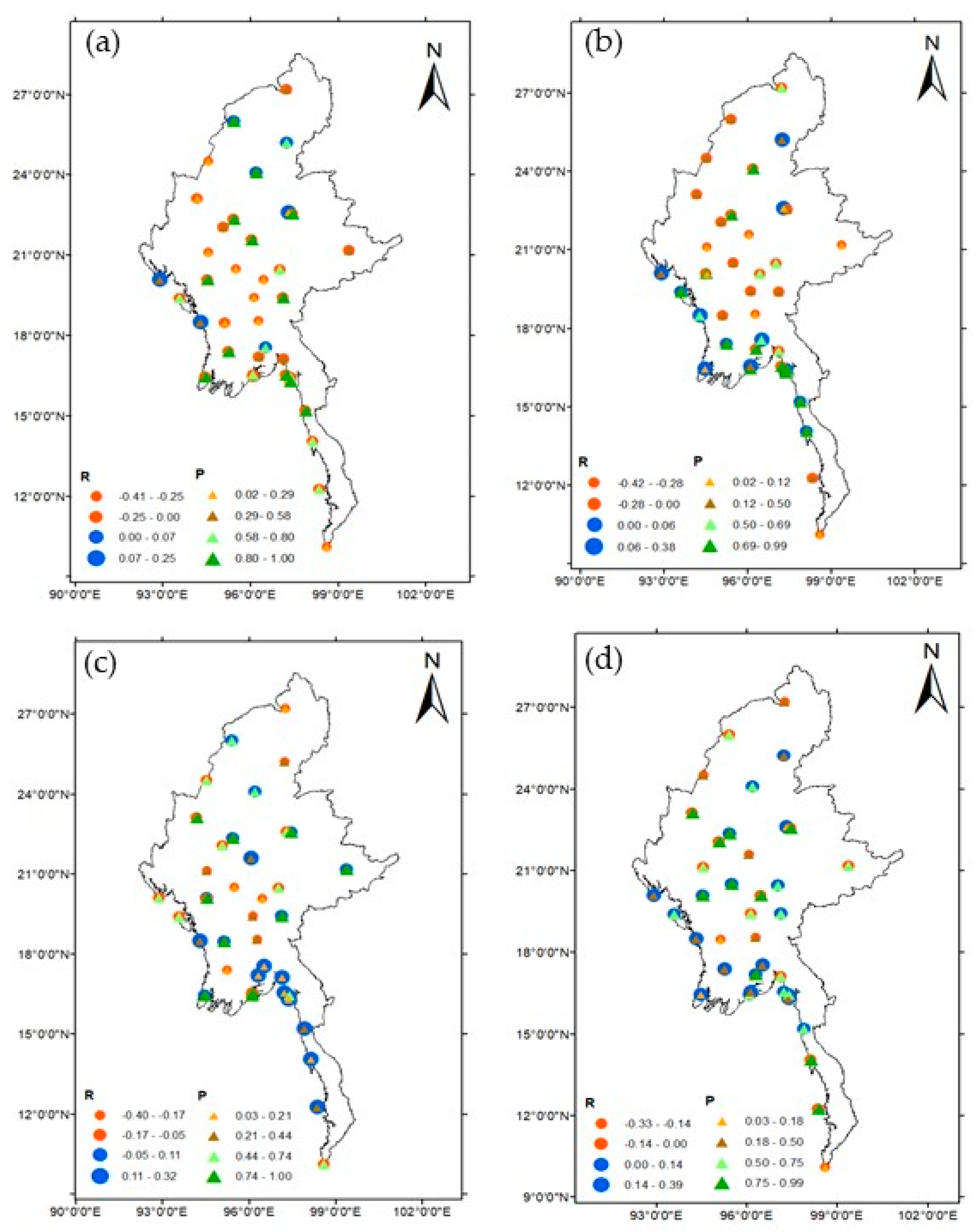
3.3. Correlation Analysis of SPEI and Its Key Mechanisms

To understand the underlying remote drivers contributing to the drought evolution across Myanmar, we examine the link between droughts evolution and some key atmospheric circulation drivers. Here, we focused on two drivers, namely, El Niño-Southern Oscillation (ENSO) and Indian Ocean Dipole (IOD), based on a recommendation from past studies [75], to understand the spatial and temporal dynamics.

To calculate the spatial pattern, correlation analysis was performed at annual and seasonal scales. Figure 9 and Figure S1 present correlation and their significance between droughts, ENSO and IOD, respectively.

In Figure 9a, we observe the correlation coefficients between SPEI the annual values and Niño-3.4 index. The correlation results were positive and significant (i.e., ≥ 0.58, p < 0.05) mainly in the deltaic zone along the coastal region.

Figure 9b–d show station correlation for individual seasons. In general, the spatial patterns for annual and August-October (ASO) show similar patterns but differences in levels of significance. However, we observed that the spatial patterns for MJJ and the entire monsoon season (MJJASO) were similar in both magnitude of correlation coefficients and significance levels.

The western hilly and central dry eco-zones showed lower but negative correlation values for annual (i.e., ≥0.25, p < 0.05) followed by ASO (≤0.42, p < 0.05) and mixed results in the northern and eastern hilly eco-zones. The mixed results in those regions range from high positive (and highly significant) to moderately negative (significant).

In Figure S1a–d, the correlation coefficients between annual (Figure S1a) and seasonal SPEI (Figure S1b–d) and IOD are similar (in R-values) but with opposite signs of the significance level. In particular, we observe that eco-zones with highly significant values in ENSO showed low to moderate values for IOD in annual and different seasons.

Secondly, we performed correlation at each station with ENSO and IOD on an annual scale to understand the temporal dynamics.

Table 2. Temporal correlation between seasonal precipitation and ENSO, and IOD during 1986–2015.

	ENSO	IOD
Annual	−0.13 (0.493)	0.43 (0.017)
MJJ	−0.07 (0.695)	0.35 (0.060)
ASO	0.16 (0.384)	0.46 (0.011)
MJJASO	0.05 (0.811)	0.44 (0.014)

Probability values are shown in parentheses.

shows the correlation (R) between SPEI and ENSO and IOD.

The results show that the SPEI influence was mainly explained by ENSO and IOD episodes. We observe that an overall weak correlation value (no significant level) concerning ENSO (≥0.15, p > 0.05) while in IOD results (≥0.46, p < 0.05), the correlation coefficient results moderate and statistically significant at 5% level. Generally, the SPEI influence was mainly explained by changes in IOD in the region since the correlation values were reported at 0.46 of SPEI variations (Table 2).

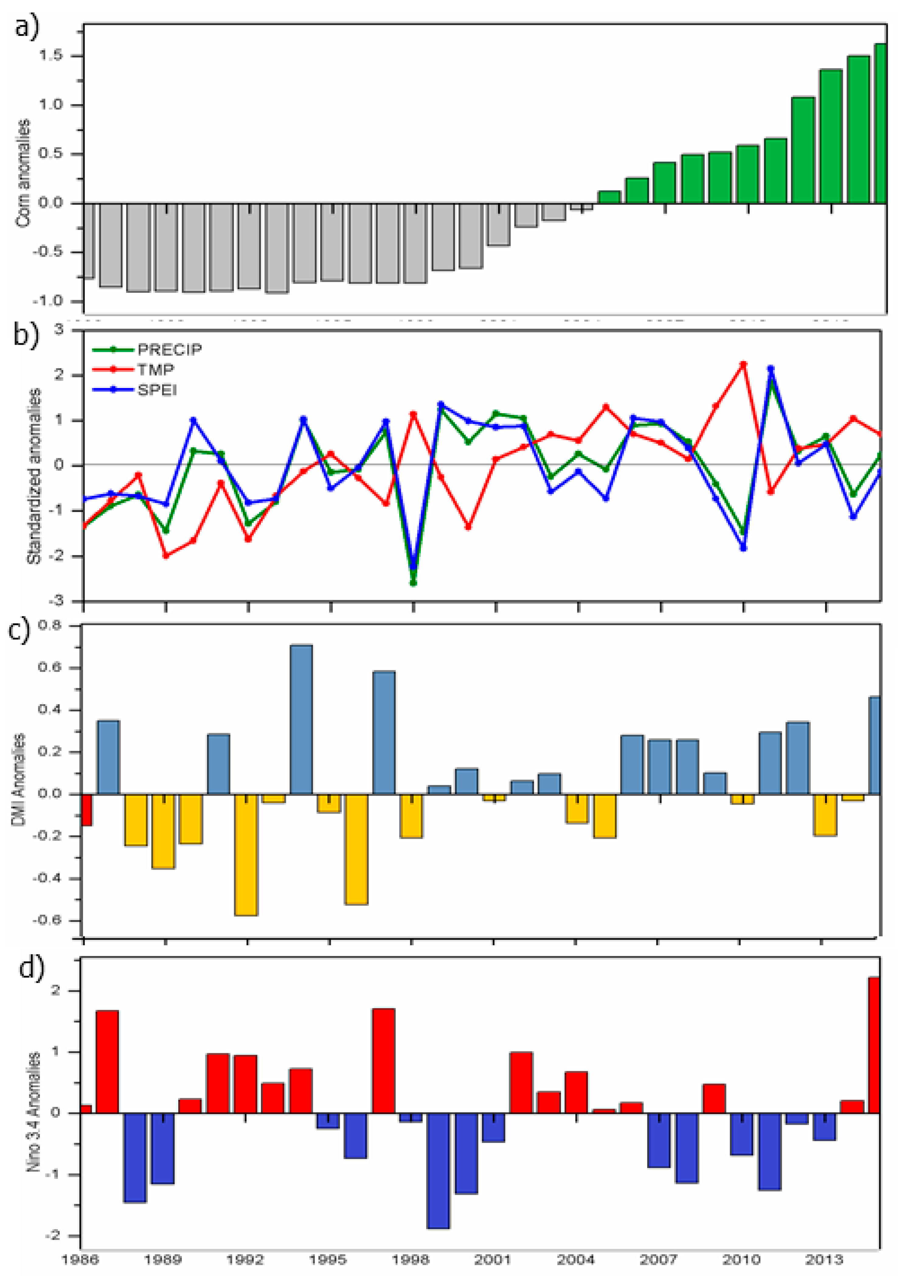
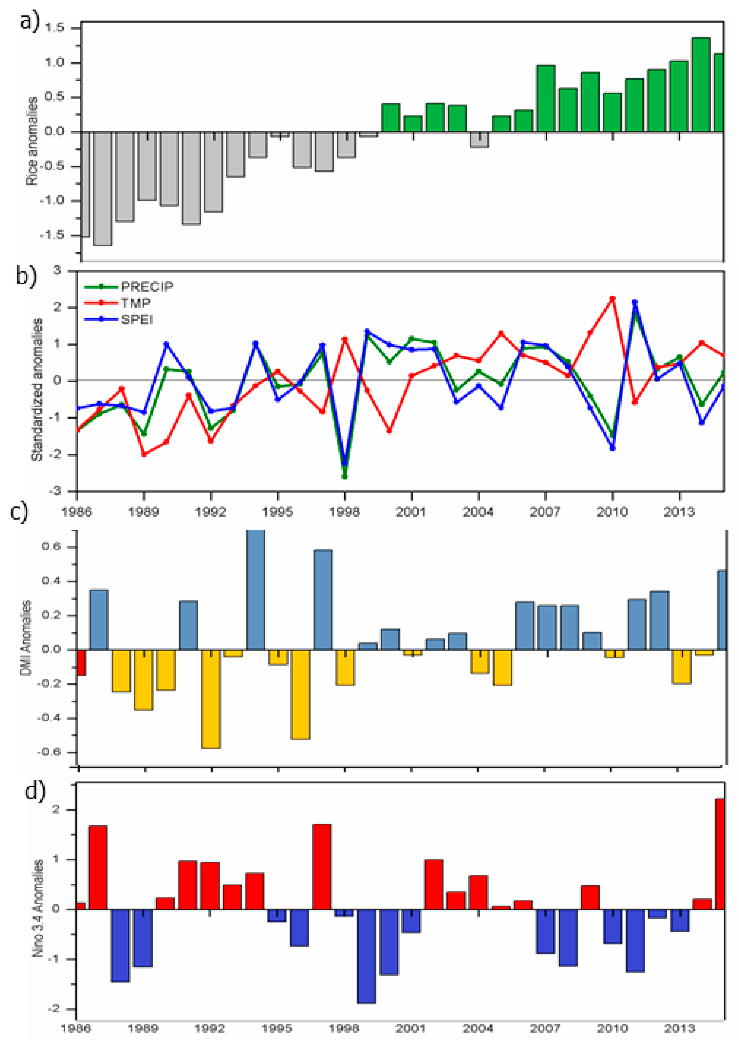
3.4. Crop Productions and Its Influencing Factors

To describe the major agriculture characteristics of Myanmar, we present the temporal distribution of the three major crops grown in Myanmar. The crop annual statistics data were downloaded from the FAOSTAT database [65]. The annual distributions of the major three crops grown in Myanmar from 1986 to 2015 are presented in Figure 10.

Figure 10a presents the production and total area statistics of rice in Myanmar. Generally, from 1986 to 2015, rice shown a steady increase in production (Figure 10, red line graph) and a corresponding increase in rice area grown (Figure 10, bar graph). We observe steady rice production (area grown) move from 7075 × 10³ MT (4603 HA) in 1986 to 13,200 × 10³ MT (7040 HA) in 2015.

On the other hand, corn production (area grown) rose from 303 × 10³ MT (229 HA) in 1986 to 2450 × 10³ MT (585 HA) in 2015 in Figure 10b. On the contrary, wheat production (area grown) decreased from 206 × 10³ MT (131HA) in 1986 to 95 × 10³ MT (62HA) in 2015 in Figure 10c.

The result in Figure 10 makes rice as the first extensive crop grown followed by corn production in Myanmar (Figure 10a). This result is not surprising as rice production the most geographically ubiquitous crop in Myanmar (as well as south and southeast Asia). In addition, the Figure 10b result makes corn is the second major crop grown in Myanmar from 1986 to 2015 consistent with FAO reports [76].

In addition, to understand possible climate changes implications on crop production, we conducted two separate analyses; the composite and correlational analysis. Reasons for selecting these two analyses is well articulated in [4,77]. Here, the study explored how to combined historical observations of crop production and weather and climate variables to explains crop production. The period of our analysis was based on annual timescales from 1986 to 2015 consistent with the period of weather station acquired.

For ease of comparison, the study made a composite of annual SPEI (in Figure 5c), precipitation (Figure 4a), temperature (Figure 4b) anomalies to present as shown in Figure 10b, Figure 11b and Figure S3b while the remaining figures were new information.

Figure 11 shows the composite analysis of rice production anomalies with multiple influencing factors (i.e., SPEI, precipitation anomalies, temperature anomalies, teleconnections).

Generally, we observed a significant decrease in crop production from 1986 to 1999 for rice (Figure 11a), corn (Figure 12a) and Wheat (Figure S3a) as compared to 2000–2015. However, we observed that two contrasting periods stood out (i.e., 1986–1999 and 2002–2015) consistent to relatively, the period of dryness (wetness) from 1986–1999 (2000–2015) in Figure 4a and Figure 5c.

From both Figure 4a and Figure 5c we observed similar dryness periods (1986–1989, 1992/3, 1995/6, 1998, 2003–2005) varying from mild to moderate drought (with values <−1.5) and relatively wetness periods in the remaining periods. The most severe drought event on record occurred from 1998, 2005, 2008, 2010, 2013 in Figure 5 corroborates with the period of crop production reduction (Figure 11, Figure 12 and Figure S3).

Also, Figure 11b,c, Figure 12b,c and Figure S3b,c) showed the composite analysis of El Niño episodes (2001, 2002, 2003) and La Niña episodes (2010–2013 which occurred over three conservative ENSO years within the period 1986 to 2015, which has implications on atmospheric water supply (i.e., precipitation) and heat stress (temperature rise) over the regions. This result is consistent with the previous literature [78,79]. Similar results across the globe are reported in the IPCC AR4&5 reports [1,80] with a corresponding threat to different sectors of the society (e.g., agriculture, economic and social)

In addition, crops growth is sensitive to different aspects of the climate and under the current warming climate, this study explored the relative importance of different climatic factors on the three-crop production across Myanmar. We conducted correlational to helps us to understand which specific crop types were significantly exposed to dryness and wetness conditions following similar analysis in [81]. The main difference in our study analysis from [71], is the including of multiple datasets (i.e., long term (annual) and short (i.e., seasonal (MJJ, ASO and MJJASO)).

The selection of the seasons was done following the three cropping seasons (summer, monsoon, and winter) of Myanmar. The summer season goes February–May, while monsoon is normally June-September, and winter is October–January [49,82]. In

Table 3. Correlation coefficients between crop production anomalies (CPA) and climate and teleconnection variables from 1986–2015.

Stat. Index	CPA	SPEI (Annual)	SPEI (MJJ)	SPEI (ASO)	SPEI (MJJASO)	PRECIP	TEMP	ENSO	IOD
R	Corn	0.280	0.320	0.390	0.170	0.46 *	0.42 *	−0.151	+0.203
	Wheat	0.020	0.160	−0.03	0.110	0.09	0.31	−0.249	−0.133
	Rice	0.050	−0.040	0.120	−0.040	0.001	−0.09	−0.156	−0.004
	AVG	0.117	0.147	0.160	0.080	0.046	0.110	−0.185	0.022

* The following denotes the anomalies of CPA = crop production; TEMP = temperature; Precip = precipitation; R = correlation co-efficient; AVG = Average.

, we presented the correlation results of crop anomalies with the multiple datasets.

From Table 3, the results showed that the relative importance of each of the climate variables vary in their response to crop production anomalies. We observed that the correlation values ranging from −0.009 to 0.460 (Table 3). Although the R values were relatively low this does not mean that climate variables in Myanmar do not have a trend, but just that the trend stays within the limits of natural variability during the time range of our analysis. This assertation is consistent studies conducted at global scale [83] and regional scales [46,84].

Generally, we found that SPEI (annual) the accounted for 0.12 of the combined effect on the three-crop production variability. This suggest that over the period, the variations of these three-crop production are explained by changes in SPEI in the region. However, the individual coefficient values varied considerably with Corn (R = 0.280) showed higher variability, followed by Rice (R = 0.02) and Wheat (0.02).

On the other hand, when we examined the shorter time scales drought indices (MJJ, ASO), we observed that the average value increased in MJJ (R = 0.147) and ASO (R = 0.160) for the three crops but lower for MJJASO (R = 0.080) suggesting that the crops are most slightly correlated in MJJ and ASO than on longer time scales. This result corroborates with previous studies that suggest that shorter time scale is appropriate for agricultural drought monitoring [85].

Also, we found among the three crops, corn production anomalies increase in MJJ (R = 0.320) and ASO (R = 0.390) but lower in MJJASO (R = 0.170). The results for MJJ and ASO for corn production are not surprising these months are the most critical cropping months (i.e., the early monsoon season) which correspond to the corn planting to early reproductive stage (tasseling/silking) in Myanmar cropping calendar. The result is consistent with previous studies in the region [82] as the phenology of these crops explains why their anomalies correlate most closely with MJJ than the rest. This result is consistent with findings of [69,71,72].

On the contrary, wheat showed that positive correlation in MJJ (R = 0.160) and negative R = −0.03 in ASO. The ASO is late monsoon season in Myanmar and correspond to harvesting time for wheat. Rice result showed that negative correlation in MJJ (R = −0.04) and positive R = 0.12 in ASO.

We observe precipitation, and temperature anomalies show the highest correlation with corn production anomalies, followed by Wheat and Rice (Table 3).

The PRECIP positive relationship was considerably weaker (R = 0.046) than in TEMP (R ≤ 0.110) (Table 3) in the region suggesting that TEMP is a limiting driver of crop production anomalies than PRECIP in the region.

Crops are known to be impacted by precipitation and temperature variability [86]. Table 3 shows corn production anomalies showed the highest correlation values (in both PRECIP and TEMP) than Wheat and Rice. Note that rice shows a negative but weaker correlation of with TEMP (Table 3, R = −0.09). Similar results were shown for corn for SPEI at both annual and seasonal scales (Table 3). This result is not surprising as corn is sensitive to water stress (i.e., both water supply and demand, respectively) at five main phenological stages of corn growth, although their sensitivity varied at each stage [87].

In Table 3, the results of wheat showed responds to TEMP (R = 0.34) than PRECIP (R = 0.09). These results suggest respond to heat stress (i.e., TEMP) than PRECIP. This result finding is in line with Semenov and Shewry [88]. In addition, the wheat relationship with TEMP is not surprising as this result is consistent with a study by Lobell et al. [46] in India.

Generally, crops responds to TEMP, when coincides with flowering, impacting the ageing of leaves and accelerates crops towards maturity consistent with [46,79]. Schelenker and Roberts [84], found high TEMP influences crops yields in the US. TEMP may be a more significant driver of crop production than precipitation. However, more detailed analysis is needed to understand this mechanism at field scale. Further studies should use longer time period and/or gridded datasets to confirm this analysis

ENSO and IOD play key role in the crop production cycle. Results of CPA with ENSO and IOD is shown in Table 3. ENSO and IOD had a significant positive correlation coefficient (R) with corn (R = 0.203) but negative with wheat (R = −0.133) and rice (R = −0.004), respectively. This result agrees well with that ENSO and IOD cycle impacts crop via controls on precipitation. This result corroborates with previous studies that suggest ENSO and IOD cycles impacts crop productions [89,90]. We acknowledge that quantifying and comparing the relationship between drought losses across time is challenging as crop productions is not controlled only by weather and climate factors but by other factors such as scientific and technological advances (e.g., improvements in plant genetics, fertilizer, pesticides, and irrigation facilities). In addition, the spatial sampling of the meteorological stations could explain the low correlation values. For example, the meteorological stations at a given point is not as representative of the entire area. The spatial sampling of the localized rain cells may occasionally poorly capture precipitation event to influence the correlation results. This assertation is consistent with [91]. We recommend future studies may consider using gridded datasets to examine this phenomenon. However, overall, this study has demonstrated that the fluctuations of crop production may be explained by weather and climate factors.

4. Summary and Conclusions

The long-term spatial distribution (1986–2015) annual mean of Temp and Precip was analyzed. Overall, the Precip and Temp follows the topography. The hilly region received less Temp and coastal and central dry zone received high Temp. The Rakhine coastal and southern Myanmar coastal received highest Precip due to the modulated by summer monsoon season over Southeast Asia. The annual variation in Temp and Precip over Myanmar showed that the Temp pattern is bi-modal, with the highest peak in April (summer season) and the second in October (late monsoon period). Moreover, a unimodal precipitation pattern corresponding to the summer monsoon season from May-October is observed. The highest Precip peak is found in June-July-August. A distinctive characteristic in spatial Temp and Precip patterns (Figure 3) showed that the high Precip as oppose low Temp in the region is modulated by Indian monsoon season over Myanmar.

Also, the inter-annual variation in Precip and Temp standardized anomalies presented an opposite variation between the two variables (Figure 4). The high (low) precipitation value coincides with low (high) temperature value, however, overall, both variables exhibited an increasing trend. The analysis of SPEI over Myanmar was presented for multiple time scales of 3,6, and 12 months, respectively (Figure 5). Overall, the temporal patterns for SPEI-3, SPEI-6 and SPEI-12, and the patterns for years with dryness and wetness are similar however differences in their relative magnitudes can be noted. It is found that short-term climate conditions (SPEI-3 and SPEI-6) in Figure 5a,b are closer to each other than that of long-term climatic conditions (SPEI-12) with 1998 recorded as an extreme drought year in the SPEI-3 and SPEI-6 and SPEI-12. On the other hand, the SPEI-3 showed the highest occurrence of droughts, followed by SPEI-6. SPEI-12 showed the lowest percentage of extreme droughts in terms of drought intensity (Table 1). SPEI-3 show dominant severe droughts over very wet conditions between 1986 and 2015.

We examined how ENSO and IOD contributes to the drought evolution on correlation analysis performed at annual and seasonal scales. The study found that the ENSO results were positive and significant mainly in the deltaic zone along the coastal region annual and August-October (ASO). While, the interior areas (i.e., the western hilly and central dry eco-zones) showed lower but negative correlation values for annual and ASO. Similarly, the IOD are similar (in R-values) but with opposite signs of the significance level. In particular, we observe that eco-zones with highly significant values in ENSO showed low to moderate values for IOD in annual and different seasons.

Within the agricultural sector, droughts reduce soil-water availability, thus, affecting crop failures and pasture losses. If drought occurrences last longer then it may severely impact growth of crops. There is evidence to show that these severe droughts have impacted crop yield thus, threatening regional food security in regions with rain-fed agricultural system. The potential influence of climate variability on crop production would be its sensitivity mainly to rainfall and temperature variability.

The study used both composite and correlational analysis to understand possible climate changes implications on crop production. The composite analysis of crop production anomalies analyzed with multiple influencing factors (i.e., SPEI, precipitation anomalies, temperature anomalies, teleconnections). A significant decrease in crop production from 1986 to 1999 was observed for all crops compared to 2000–2015 consistent with the relative dryness and wetness conditions over the period. The two contrasting periods stood out (i.e., 1986–1999 and 2002–2015) consistent to the period of dryness (wetness) from 1986–1999 (2000–2015). Note that these periods were characterized with dryness periods (1986–1989, 1992/3, 1995/6, 1998, 2003–2005) varying from mild to moderate drought (with values <−1.5) and relatively wetness periods in the remaining periods. Similarly, the composite analysis of El Nino episodes (2001, 2002, 2003) and La Niña episodes (2010–2013 which occurred over three conservative ENSO years within the period 1986 to 2015, which has implications on atmospheric water supply (i.e., precipitation) and heat stress (temperature rise) over the regions.

The correlational helps us to understand which specific crop types were significantly exposed to dryness and wetness conditions. Crop growth is sensitive to different aspects of the climate and under the current warming climate. Based on the three cropping seasons (summer, monsoon, and winter) of Myanmar, the correlation results of crop anomalies with the multiple datasets showed interesting results. The results showed that the relative importance of each of the climate variables vary in their response to crop production anomalies. The correlation values ranging from −0.009 to 0.460. Although the R values were relatively low this does not mean that climate variables in Myanmar do not have a trend, but just that the trend stays within the limits of natural variability during the time range of our analysis. This assertation is consistent studies conducted at global scale and regional scales.

Overall, the variations of these three-crop production are explained by changes in the multiple datasets used in the region. Here, our analysis focused on how the climate change signal on crop production anomalies from 1986 to 2015 to understand with sufficient detail the processes involved in potential crop production changes. We urge readers to interpret this result findings caution as crop production declines are not driven by a single event, but rather result from a confluence of other factors including farm management practices adopted, seed quality used, technological investments inputs, crop price fluctuations, research and development, etc. We have identified the spatiotemporal variation of drought and its impacts on agriculture. This results analysis could provide policy makers and stakeholders with scientific information regarding which agricultural areas are most vulnerable and sensitive to drought. We recommend further studies could build upon our analysis. Future studies on trend analysis should consider non-linear models that are predictive and also include physiological detail necessary to explain the processes behind the crop production–climate (teleconnection) associations. In addition, further study should study the future changes in climate and its impact on food production over the region. Particularly increasing resource constraints within the context of climate change, with decreasing water and land resources would impact food production.

References

1. IPCC. Climate Change; Cambridge University Press: Cambridge, UK; New York, NY, USA, 2014. [Google Scholar]
2. Hao, Z.; Singh, V.P. Drought characterization from a multivariate perspective: A review. J. Hydrol. 2015, 527, 668–678. [Google Scholar] [CrossRef]
3. Mishra, A.K.; Singh, V.P. A review of drought concepts. J. Hydrol. 2010, 391, 202–216. [Google Scholar] [CrossRef]
4. Nooni, I.K.; Hagan, D.F.T.; Wang, G.; Ullah, W.; Li, S.; Lu, J.; Bhatti, A.S.; Shi, X.; Lou, D.; Prempeh, N.A.; et al. Spatiotemporal Characteristics and Trend Analysis of Two Evapotranspiration-Based Drought Products and Their Mechanisms in Sub-Saharan Africa. Remote Sens. 2021, 13, 533. [Google Scholar] [CrossRef]
5. WMO. Guide to Climatological Practices. Weather, Climate and Water; WMO: Geneva, Switzerland, 2011. [Google Scholar]
6. Wilhite, D.A.; Glantz, M.H. Understanding: The Drought Phenomenon: The Role of Definitions. Water Int. 1985, 10, 111–120. [Google Scholar] [CrossRef] [Green Version]
7. Wilhite, D.A.; Svoboda, M.D.; Hayes, M.J. Understanding the complex impacts of drought: A key to enhancing drought mitigation and preparedness. Water Resour. Manag. 2007, 21, 763–774. [Google Scholar] [CrossRef] [Green Version]
8. Piao, S.; Ciais, P.; Huang, Y.; Shen, Z.; Peng, S.; Li, J.; Zhou, L.; Liu, H.; Ma, Y.; Ding, Y.; et al. The impacts of climate change on water resources and agriculture in China. Nature 2010, 467, 43–51. [Google Scholar] [CrossRef]
9. Van Dijk, A.I.J.M.; Beck, H.E.; Crosbie, R.; De Jeu, R.A.M.; Liu, Y.Y.; Podger, G.M.; Timbal, B.; Viney, N. The Millennium Drought in southeast Australia (2001–2009): Natural and human causes and implications for water resources, ecosystems, economy, and society. Water Resour. Res. 2013, 49, 1040–1057. [Google Scholar] [CrossRef]
10. Vicente-Serrano, S.M.; Beguería, S.; Lorenzo-Lacruz, J.; Camarero, J.J.; Lopez-Moreno, I.; Azorin-Molina, C.; Revuelto, J.; Morán-Tejeda, E.; Sanchez-Lorenzo, A. Performance of Drought Indices for Ecological, Agricultural, and Hydrological Applications. Earth Interact. 2012, 16, 1–27. [Google Scholar] [CrossRef] [Green Version]
11. Heim, R.R. A Review of Twentieth-Century Drought Indices Used in the United States. Bull. Am. Meteorol. Soc. 2002, 83, 1149–1166. [Google Scholar] [CrossRef] [Green Version]
12. Yihdego, Y.; Vaheddoost, B.; Al-Weshah, R. Drought indices and indicators revisited. Arab. J. Geosci. 2019, 12, 69. [Google Scholar] [CrossRef]
13. Palmer, W. Meteorological Drought; US Weather Bureau: Washington, DC, USA, 1965.
14. Sheffield, J.; Wood, E.; Roderick, M. Little change in global drought over the past 60 years. Nature 2012, 491, 435–438. [Google Scholar] [CrossRef]
15. Dai, A. Characteristics and trends in various forms of the Palmer Drought Severity Index during 1900. J. Geophys. Res. Space Phys. 2011, 116. [Google Scholar] [CrossRef] [Green Version]
16. Dai, A. Increasing drought under global warming in observations and models. Nat. Clim. Chang. 2012, 3, 52–58. [Google Scholar] [CrossRef]
17. Dutta, R. Drought Monitoring in the Dry Zone of Myanmar using MODIS Derived NDVI and Satellite Derived CHIRPS Precipitation Data. Sustain. Agric. Res. 2018, 7, 46. [Google Scholar] [CrossRef] [Green Version]
18. Dai, A.; Trenberth, K.E.; Qian, T. A Global Dataset of Palmer Drought Severity Index for 1870–2002: Relationship with Soil Moisture and Effects of Surface Warming. J. Hydrometeorol. 2004, 5, 1117–1130. [Google Scholar] [CrossRef]
19. McKee, T.B.; Doesken, N.J.; Kleist, J. The relationship of drought frequency and duration to time scales. In Proceedings of the Eighth Conference on Applied Climatology, Anaheim, CA, USA, 17–23 January 1993; pp. 174–184. [Google Scholar]
20. Alley, W.M. The Palmer drought severity index: Limitations and applications. J. Appl. Meteor. 1984, 23, 1100–1109. [Google Scholar] [CrossRef] [Green Version]
21. Mechiche-Alami, A.; Abdi, A.M. Agricultural productivity in relation to climate and cropland management in West Africa. Sci. Rep. 2020, 10, 1–10. [Google Scholar] [CrossRef]
22. Vicente-Serrano, S.M.; Beguería, S.; Lopez-Moreno, I. A Multiscalar Drought Index Sensitive to Global Warming: The Standardized Precipitation Evapotranspiration Index. J. Clim. 2010, 23, 1696–1718. [Google Scholar] [CrossRef] [Green Version]
23. Li, W.-G.; Yi, X.; Hou, M.-T.; Chen, H.-L.; Chen, Z.-L. Standardized precipitation evapotranspiration index shows drought trends in China. Chin. J. Eco-Agric. 2012, 20, 643–649. [Google Scholar] [CrossRef]
24. Jia, Y.; Zhang, B.; Ma, B. Daily SPEI Reveals Long-term Change in Drought Characteristics in Southwest China. Chin. Geogr. Sci. 2018, 28, 680–693. [Google Scholar] [CrossRef] [Green Version]
25. Kambombe, O.; Ngongondo, C.; Eneya, L.; Monjerezi, M.; Boyce, C. Spatio-temporal analysis of droughts in the Lake Chilwa Basin, Malawi. Theor. Appl. Clim. 2021, 144, 1219–1231. [Google Scholar] [CrossRef]
26. Li, S.; Yao, Z.; Wang, R.; Liu, Z. Dryness/wetness pattern over the Three-River Headwater Region: Variation characteristic, causes, and drought risks. Int. J. Clim. 2019, 40, 3550–3566. [Google Scholar] [CrossRef]
27. Liu, C.; Yang, C.; Yang, Q.; Wang, J. Spatiotemporal drought analysis by the standardized precipitation index (SPI) and standardized precipitation evapotranspiration index (SPEI) in Sichuan Province, China. Sci. Rep. 2021, 11, 1–14. [Google Scholar] [CrossRef]
28. Ma, B.; Zhang, B.; Jia, L.; Huang, H. Conditional distribution selection for SPEI-daily and its revealed meteorological drought characteristics in China from 1961 to 2017. Atmos. Res. 2020, 246, 105108. [Google Scholar] [CrossRef]
29. Li, X.; Huang, W.-R. How long should the pre-existing climatic water balance be considered when capturing short-term wetness and dryness over China by using SPEI? Sci. Total Environ. 2021, 786, 147575. [Google Scholar] [CrossRef]
30. Tefera, A.S.; Ayoade, J.O.; Bello, N.J. Comparative analyses of SPI and SPEI as drought assessment tools in Tigray Region, Northern Ethiopia. SN Appl. Sci. 2019, 1, 1265. [Google Scholar] [CrossRef] [Green Version]
31. Wang, Q.; Shi, P.; Lei, T.; Geng, G.; Liu, J.; Mo, X.; Li, X.; Zhou, H.; Wu, J. The alleviating trend of drought in the Huang-Huai-Hai Plain of China based on the daily SPEI. Int. J. Clim. 2015, 35, 3760–3769. [Google Scholar] [CrossRef]
32. Wang, Q.; Zeng, J.; Qi, J.; Zhang, X.; Zeng, Y.; Shui, W.; Xu, Z.; Zhang, R.; Wu, X.; Cong, J. A multi-scale daily SPEI dataset for drought characterization at observation stations over mainland China from 1961 to 2018. Earth Syst. Sci. Data 2021, 13, 331–341. [Google Scholar] [CrossRef]
33. Wang, W.; Guo, B.; Zhang, Y.; Zhang, L.; Ji, M.; Xu, Y.; Zhang, X.; Zhang, Y. The sensitivity of the SPEI to potential evapotranspiration and precipitation at multiple timescales on the Huang-Huai-Hai Plain, China. Theor. Appl. Clim. 2020, 143, 87–99. [Google Scholar] [CrossRef]
34. Wu, M.; Li, Y.; Hu, W.; Yao, N.; Li, L.; Liu, D.L. Spatiotemporal variability of standardized precipitation evapotranspiration index in mainland China over 1961–2016. Int. J. Clim. 2020, 40, 4781–4799. [Google Scholar] [CrossRef]
35. Zhang, R.; Chen, T.; Chi, D. Global Sensitivity Analysis of the Standardized Precipitation Evapotranspiration Index at Different Time Scales in Jilin Province, China. Sustainability 2020, 12, 1713. [Google Scholar] [CrossRef] [Green Version]
36. Katchele, O.F.; Ma, Z.-G.; Yang, Q.; Batebana, K. Comparison of trends and frequencies of drought in central North China and sub-Saharan Africa from 1901 to 2010. Atmos. Ocean. Sci. Lett. 2017, 10, 418–426. [Google Scholar] [CrossRef] [Green Version]
37. Lobell, D.B.; Schlenker, W.; Costa-Roberts, J. Climate Trends and Global Crop Production Since 1980. Science 2011, 333, 616–620. [Google Scholar] [CrossRef] [Green Version]
38. Fahad, S.; Bajwa, A.; Nazir, U.; Anjum, S.A.; Farooq, A.; Zohaib, A.; Sadia, S.; Nasim, W.; Adkins, S.; Saud, S.; et al. Crop Production under Drought and Heat Stress: Plant Responses and Management Options. Front. Plant Sci. 2017, 8, 1147. [Google Scholar] [CrossRef] [Green Version]
39. Geng, G.; Wu, J.; Wang, Q.; Lei, T.; He, B.; Li, X.; Mo, X.; Luo, H.; Zhou, H.; Liu, D. Agricultural drought hazard analysis during 1980–2008: A global perspective. Int. J. Clim. 2015, 36, 389–399. [Google Scholar] [CrossRef]
40. Wang, Q.; Wu, J.; Lei, T.; He, B.; Wu, Z.; Liu, M.; Mo, X.; Geng, G.; Li, X.; Zhou, H.; et al. Temporal-spatial characteristics of severe drought events and their impact on agriculture on a global scale. Quat. Int. 2014, 349, 10–21. [Google Scholar] [CrossRef]
41. Hunt, E.D.; Svoboda, M.; Wardlow, B.; Hubbard, K.; Hayes, M.; Arkebauer, T. Monitoring the effects of rapid onset of drought on non-irrigated maize with agronomic data and climate-based drought indices. Agric. For. Meteorol. 2014, 191, 1–11. [Google Scholar] [CrossRef]
42. Páscoa, P.; Gouveia, C.M.; Russo, A.; Trigo, R.M. The role of drought on wheat yield interannual variability in the Iberian Peninsula from 1929 to 2012. Int. J. Biometeorol. 2016, 61, 439–451. [Google Scholar] [CrossRef]
43. Karim, R.; Rahman, M.A. Drought risk management for increased cereal production in Asian Least Developed Countries. Weather. Clim. Extrem. 2015, 7, 24–35. [Google Scholar] [CrossRef] [Green Version]
44. Knox, J.; Hess, T.; Daccache, A.; Wheeler, T. Climate change impacts on crop productivity in Africa and South Asia. Environ. Res. Lett. 2012, 7, 034032. [Google Scholar] [CrossRef]
45. Liu, X.; Pan, Y.; Zhu, X.; Yang, T.; Bai, J.; Sun, Z. Drought evolution and its impact on the crop yield in the North China Plain. J. Hydrol. 2018, 564, 984–996. [Google Scholar] [CrossRef]
46. Lobell, D.; Sibley, A.M.; Ortiz-Monasterio, J.I. Extreme heat effects on wheat senescence in India. Nat. Clim. Chang. 2012, 2, 186–189. [Google Scholar] [CrossRef]
47. Madadgar, S.; AghaKouchak, A.; Farahmand, A.; Davis, S.J. Probabilistic estimates of drought impacts on agricultural production. Geophys. Res. Lett. 2017, 44, 7799–7807. [Google Scholar] [CrossRef]
48. Mangani, R.; Tesfamariam, E.; Bellocchi, G.; Hassen, A. Modelled impacts of extreme heat and drought on maize yield in South Africa. Crop. Pasture Sci. 2018, 69, 703. [Google Scholar] [CrossRef]
49. Oo, A.T.; Van Huylenbroeck, G.; Speelman, S. Measuring the Economic Impact of Climate Change on Crop Production in the Dry Zone of Myanmar: A Ricardian Approach. Climate 2020, 8, 9. [Google Scholar] [CrossRef] [Green Version]
50. FAO. The State of Food and Agriculture 2016; Food and Agriculture of the United Nations: Rome, Italy, 2016. [Google Scholar]
51. FAO. FAOSTAT on the UN, Myanmar; Food and Agriculture Organization of the United Nations (FAO): Rome, Italy, 2018; Available online: http://faostat.fao.org/CountryProfiles/Country_Profile/Direct.aspx?lang=en&area=28 (accessed on 30 May 2021).
52. Gebreegziabher, Z.; Mekonnen, A.; Bekele, R.D.; Zewdie, S.A.; Kassahun, M.M. Crop-Livestock Inter-Linkages and Climate Change Implications for Ethiopia’s Agriculture. Environment for Development Discussion Paper Series EfD DP 13–14; Springer: Cham, Switzerland, 2013; 32p. [Google Scholar] [CrossRef]
53. Sein, Z.M.; Ullah, I.; Saleem, F.; Zhi, X.; Syed, S.; Azam, K. Interdecadal Variability in Myanmar Rainfall in the Monsoon Season (May–October) Using Eigen Methods. Water 2021, 13, 729. [Google Scholar] [CrossRef]
54. Sein, Z.M.; Ullah, I.; Syed, S.; Zhi, X.; Azam, K.; Rasool, G. Interannual Variability of Air Temperature over Myanmar: The Influence of ENSO and IOD. Climate 2021, 9, 35. [Google Scholar] [CrossRef]
55. Sein, Z.M.M.; Zhi, X. Interannual variability of summer monsoon rainfall over Myanmar. Arab. J. Geosci. 2016, 9, 469. [Google Scholar] [CrossRef]
56. Paing Oo, S. Farmers’ Awareness of the Low Yield of Conventional Rice Production in Ayeyarwady Region, Myanmar: A Case Study of Myaungmya District. Agriculture 2020, 10, 26. [Google Scholar] [CrossRef] [Green Version]
57. Matsuda, M. Upland Farming Systems Coping with Uncertain Rainfall in the Central Dry Zone of Myanmar: How Stable is Indigenous Multiple Cropping Under Semi-Arid Conditions? Hum. Ecol. 2013, 41, 927–936. [Google Scholar] [CrossRef]
58. DIVA-GIS Homepage. Download Data by Country. Available online: https://diva-gis.org/ (accessed on 30 May 2021).
59. Department of Meteorology and Hydrology, Ministry of Transport. Myanmar’s National Adaptation Programme of Action (NAPA) to Climate Change; The Republic Union of Myanmar, National Environmental Conservation Committee, Ministry of Environmental Conservation and Forestry: Nay Pyi Taw, Myanmar, 2012; pp. 1–126.
60. Marchant, R.; Richer, S.; Boles, O.; Capitani, C.; Mustaphi, C.C.; Lane, P.; Prendergast, M.E.; Stump, D.; De Cort, G.; Kaplan, J.O.; et al. Drivers and trajectories of land cover change in East Africa: Human and environmental interactions from 6000 years ago to present. Earth-Sci. Rev. 2018, 178, 322–378. [Google Scholar] [CrossRef]
61. Yi, T.; Hla, W.M.; Htun, A.K. Drought Conditions and Management Strategies in Myanmar. In Report of the Department of Meteorology and Hydrology, Myanmar; Department of Meteorology and Hydrology, Ministry of Transport: Nay Pyi Taw, Myanmar, 2014. [Google Scholar]
62. UNDP. Enhancing Capacities for Climate Risk Management in Myanmar’s Dry Zone through Climate Information and Services; UNDP: New York, NY, USA, 2018; Available online: https://www.adaptation-fund.org/ie/united-nations-development-programme-undp/ (accessed on 21 March 2021).
63. Trenberth, K.E. ENSO in the Global Climate System. In El Niño Southern Oscillation in a Changing Climate; John Wiley & Sons: Hoboken, NJ, USA, 2020; pp. 21–37. [Google Scholar]
64. NOAA, Physical Sciences Laboratory Homepge, Nino SST Indices (Nino 3.4), Mean Using Ersstv5 from CPC (Trenberth 2020) and Dipole Mode Index (DMI) HadISST1.1. Available online: https://psl.noaa.gov/data/timeseries/ (accessed on 30 May 2021).
65. FAOSTAT. FAO Statistics Data Base on the World Wide Web; FAO: Rome, Italy, 2021; Available online: http://faostat.fao.org (accessed on 19 May 2021).
66. ESRI Home. ArcGIS Desktop: Release Redlands; Environmental Systems Research Institute: Redlands, CA, USA; Available online: https://www.esri.com (accessed on 21 March 2021).
67. Thornthwaite, C.W. An Approach toward a Rational Classification of Climate. Geogr. Rev. 1948, 38, 55. [Google Scholar] [CrossRef]
68. R Development Core Team. R: A Language and Environment for Statistical Computing. R Foundation for Statistical Computing, Vienna. Available online: https://www.yumpu.com/en/document/read/6853895/r-a-language-and-environment-for-statistical-computing (accessed on 21 March 2021).
69. Mann, H.B. Nonparametric Tests Against Trend. Econometrica 1945, 13, 245. [Google Scholar] [CrossRef]
70. Nooni, I.K.; Wang, G.; Hagan, D.F.T.; Lu, J.; Ullah, W.; Li, S. Evapotranspiration and its Components in the Nile River Basin Based on Long-Term Satellite Assimilation Product. Water 2019, 11, 1400. [Google Scholar] [CrossRef] [Green Version]
71. Ullah, W.; Wang, G.; Ali, G.; Hagan, D.F.T.; Bhatti, A.S.; Lou, D. Comparing Multiple Precipitation Products against In-Situ Observations over Different Climate Regions of Pakistan. Remote Sens. 2019, 11, 628. [Google Scholar] [CrossRef] [Green Version]
72. Ullah, W.; Wang, G.; Lou, D.; Ullah, S.; Bhatti, A.S.; Karim, A.; Hagan, D.F.T.; Ali, G. Large-scale atmospheric circulation patterns associated with extreme monsoon precipitation in Pakistan during 1981–2014. Atmos. Res. 2021, 253, 105489. [Google Scholar] [CrossRef]
73. Sian, K.L.K.; Wang, J.; Ayugi, B.; Nooni, I.; Ongoma, V. Multi-Decadal Variability and Future Changes in Precipitation over Southern Africa. Atmosphere 2021, 12, 742. [Google Scholar] [CrossRef]
74. Bärring, L.T.; Holt, M.L.; Linderson, M.; Radziejewski, M.; Moriondo, J.; Palutikof, P. Defining dry/wet spells for point observations, observed area averages, and regional climate model grid boxes in europe. Clim. Res. 2006, 31, 35–49. [Google Scholar] [CrossRef] [Green Version]
75. Manzano, A.; Clemente, M.A.; Morata, A.; Luna, M.Y.; Beguería, S.; Vicente-Serrano, S.M.; Martín, M.L. Analysis of the atmospheric circulation pattern effects over SPEI drought index in Spain. Atmos. Res. 2019, 230, 104630. [Google Scholar] [CrossRef]
76. GIEWS/FAO. FAO/WFP Crop and Food Security Assessment Mission to Myanma; FAO: Rome, Italy; Wfp: Rome, Italy, 2016. [Google Scholar]
77. Hina, S.; Saleem, F.; Arshad, A.; Hina, A.; Ullah, I. Droughts over Pakistan: Possible cycles, precursors and associated mechanisms. Geomat. Nat. Hazards Risk 2021, 12, 1638–1668. [Google Scholar] [CrossRef]
78. Hawkins, E.; Fricker, T.E.; Challinor, A.; Ferro, C.A.T.; Ho, C.K.; Osborne, T.M. Increasing influence of heat stress on French maize yields from the 1960s to the 2030s. Glob. Chang. Biol. 2012, 19, 937–947. [Google Scholar] [CrossRef] [PubMed] [Green Version]
79. Asseng, S.; Foster, I.; Turner, N. The impact of temperature variability on wheat yields. Glob. Chang. Biol. 2011, 17, 997–1012. [Google Scholar] [CrossRef]
80. IPCC. Climate Change: The Physical Science Basis-Summary for Policymakers; IPCC: Geneva, Switzerland, 2007; p. 21. [Google Scholar]
81. Fontaine, B.; Roucou, P.; Monerie, P.-A. Changes in the African monsoon region at medium-term time horizon using 12 AR4 coupled models under the A1b emissions scenario. Atmos. Sci. Lett. 2011, 12, 83–88. [Google Scholar] [CrossRef]
82. Herridge, D.F.; Win, M.M.; Nwe, K.M.M.; Kyu, K.L.; Win, S.S.; Shwe, T.; Min, Y.Y.; Denton, M.; Cornish, P.S. The cropping systems of the Central Dry Zone of Myanmar: Productivity constraints and possible solutions. Agric. Syst. 2018, 169, 31–40. [Google Scholar] [CrossRef]
83. Ray, D.K.; Gerber, J.; MacDonald, G.; West, P. Climate variation explains a third of global crop yield variability. Nat. Commun. 2015, 6, 5989. [Google Scholar] [CrossRef] [PubMed] [Green Version]
84. Schlenker, W.; Roberts, M.J. Nonlinear temperature effects indicate severe damages to U.S. crop yields under climate change. Proc. Natl. Acad. Sci. USA 2009, 106, 15594–15598. [Google Scholar] [CrossRef] [PubMed] [Green Version]
85. Qaisrani, Z.N.; Nuthammachot, N.; Techato, K. Asadullah Drought monitoring based on Standardized Precipitation Index and Standardized Precipitation Evapotranspiration Index in the arid zone of Balochistan province, Pakistan. Arab. J. Geosci. 2021, 14, 1–13. [Google Scholar] [CrossRef]
86. Sakurai, G.; Iizumi, T.; Yokozawa, M. Varying temporal and spatial effects of climate on maize and soybean affect yield prediction. Clim. Res. 2011, 49, 143–154. [Google Scholar] [CrossRef] [Green Version]
87. Kranz, W.L.; Irmak, S.; van Donk, S.J.; Yonts, C.D.; Martin, D.L. Irrigation Management for Corn; University of Nebraska-Lincoln Extension: Lincoln, NE, USA, 2008. [Google Scholar]
88. Semenov, M.A.; Shewry, P.R. Modelling predicts that heat stress, not drought, will increase vulnerability of wheat in Europe. Sci. Rep. 2011, 1, 66. [Google Scholar] [CrossRef]
89. Liu, Y.; Yang, X.; Wang, E.; Xue, C. Climate and crop yields impacted by ENSO episodes on the North China Plain: 1956–2006. Reg. Environ. Chang. 2013, 14, 49–59. [Google Scholar] [CrossRef] [Green Version]
90. Royce, F.S.; Fraisse, C.W.; Baigorria, G.A. ENSO classification indices and summer crop yields in the Southeastern USA. Agric. For. Meteorol. 2011, 151, 817–826. [Google Scholar] [CrossRef]
91. Tetzlaff, D.; Uhlenbrook, S. Significance of spatial variability in precipitation for process-oriented modelling: Results from two nested catchments using radar and ground station data. Hydrol. Earth Syst. Sci. 2005, 9, 29–41. [Google Scholar] [CrossRef] [Green Version]
92. Zhang, Y.; Kang, S.; Ward, E.; Ding, R.; Zhang, X.; Zheng, R. Evapotranspiration components determined by sap flow and microlysimetry techniques of a vineyard in northwest China: Dynamics and influential factors. Agric. Water Manag. 2011, 98, 1207–1214. [Google Scholar] [CrossRef]
93. Goldblum, D. Sensitivity of Corn and Soybean Yield in Illinois to Air Temperature and Precipitation: The Potential Impact of Future Climate Change. Phys. Geogr. 2009, 30, 27–42. [Google Scholar] [CrossRef]
94. Quiring, S.M.; Papakryiakou, T.N. An evaluation of agricultural drought indices for the Canadian prairies. Agric. For. Meteorol. 2003, 118, 49–62. [Google Scholar] [CrossRef]
95. Wu, Z.; Huang, N.E.; Long, S.R.; Peng, C.-K. On the trend, detrending, and variability of nonlinear and nonstationary time series. Proc. Natl. Acad. Sci. USA 2007, 104, 14889–14894. [Google Scholar] [CrossRef] [Green Version]
96. Walsh, J.; Mostek, A. A Quantitative Analysis of Meteorological Anomaly Patterns Over the United States, 1900–1977. Mon. Weather Rev. 1980, 108, 615–630. [Google Scholar] [CrossRef]
Figure 1. Geoinformation of Myanmar. (a) Land surface elevation (m) and meteorological station locations; (b) landcover map [58]; (c) major rivers [58]; and (d) eco-physiographic zones [59].
Agronomy 11 01691 g001
Figure 2. Spatial distribution of (a) temperature (°C); and (b) rainfall (mm) climatology over Myanmar from 1986 to 2015.
Agronomy 11 01691 g002
Figure 3. Annual cycle of rainfall (mm) (blue) and temperature (°C) (red) averaged from 1986 to 2015.
Agronomy 11 01691 g003
Figure 4. Linear trend of annual (a) rainfall (mm); and (b) temperature (°C) anomaly over Myanmar from 1986 to2015. The red lines are the annual anomalies and the blue lines are the linear trends.
Agronomy 11 01691 g004
Figure 5. Average of SPEI from all stations (SAA) (black line) and that based on area average of climatic parameters (SBA) (red line) from 1986 to 2015 over Myanmar. The SPEI at the time scale 3-, 6- and 12-months are indicated in (ac), respectively. The p represents the significance of the correlation (r).
Agronomy 11 01691 g005
Figure 6. Spatial distribution of SPEI over Myanmar from 1986 to 2015. (a) 3-month; (b) 6-month; and (c) 12-month. Red and blue dots indicate negative and positive trends, respectively, while the black (significant at 5% confidence level) and yellow (significant at 10% confidence level) triangles indicate the probability value.
Agronomy 11 01691 g006
Figure 7. Frequency of drought occurrence of dry spells over Myanmar from 1986 to 2015. (a) Annual, (b) MJJ, (c) ASO, (d) MJJASO.
Agronomy 11 01691 g007
Figure 8. Frequency of drought occurrence of wet spells over Myanmar from 1986 to 2015. (a) Annual, (b) MJJ, (c) ASO, (d) MJJASO.
Agronomy 11 01691 g008
Figure 9. Spatial map of correlation between ENSO and (a) annual; (b) MJJ; (c) ASO; and (d) MJJASO SPEI from 1986 to 2015. The arrows denote areas where the tests were significant at the 5% level. The yellow arrow denotes no correlation; purple denotes weak correlation; the light green denotes moderate while the deep green denotes high correlation, respectively. The blue and red dots represent wet and dry, respectively.
Agronomy 11 01691 g009
Figure 10. Interannual variability of crop production (1000 MT) and harvested area (HA) for (a) Rice (b) Corn (c) Wheat in Myanmar from 1986-2015.
Agronomy 11 01691 g010
Figure 11. Interannual variability of (a) Rice production anomalies in Myanmar from 1986 to 2015 (b) Wetness and Dryness conditions expressed in three anomalies forms (green-precipitation, red-temperature, red-SPEI) (c) DMI anomalies, (d) Nino 3.4 SST anomalies during the same time period.
Agronomy 11 01691 g011
Figure 12. Same as Figure 11 but for Corn production anomalies.
Agronomy 11 01691 g012