A Centralized Routing for Lifetime and Energy Optimization in WSNs Using Genetic Algorithm and Least-Square Policy Iteration

Abstract

Q-learning has been primarily used as one of the reinforcement learning (RL) techniques to find the optimal routing path in wireless sensor networks (WSNs). However, for the centralized RL-based routing protocols with a large state space and action space, the baseline Q-learning used to implement these protocols suffers from degradation in the convergence speed, network lifetime, and network energy consumption due to the large number of learning episodes required to learn the optimal routing path. To overcome these limitations, an efficient model-free RL-based technique called Least-Square Policy Iteration (LSPI) is proposed to optimize the network lifetime and energy consumption in WSNs. The resulting designed protocol is a Centralized Routing Protocol for Lifetime and Energy Optimization with a Genetic Algorithm (GA) and LSPI (CRPLEOGALSPI). Simulation results show that the CRPLEOGALSPI has improved performance in network lifetime and energy consumption compared to an existing Centralized Routing Protocol for Lifetime Optimization with GA and Q-learning (CRPLOGARL). This is because the CRPLEOGALSPI chooses a routing path in a given state considering all the possible routing paths, and it is not sensitive to the learning rate. Moreover, while the CRPLOGARL evaluates the optimal policy from the Q-values, the CRPLEOGALSPI updates the Q-values based on the most updated information regarding the network dynamics using weighted functions.

1. Introduction

A wireless sensor network (WSN) can be defined as a collection of application-specific, low-powered, tiny devices called sensor nodes that are spatially deployed in a geographic area to monitor, collect, process, and cooperatively communicate real-time physical or environmental properties, such as temperature, sound, motion, pressure, humidity, etc. to a central device called a sink using the wireless medium [1].

The advantages of WSN technology, when compared to traditional solutions of networking, are scalability, low costs, accuracy, reliability, flexibility, and deployment ease [2]. This has made WSNs efficient in different application fields, such as military, security, environment, and healthcare. However, the quality of service (QoS) requirements posed by these applications are limited by the resource constraints of the WSN, which are low power, short transmission range, low bandwidth, low memory, and the limited processing and computing speed of the sensor nodes [3].

Basically, a wireless sensor node is a device that consists of a power unit, sensing unit, processing unit, and radio transceiver unit. The majority of the energy consumed in a sensor node is due to data communication with other sensor nodes [4]. The power unit consists of a limited energy source that supplies energy to the other units. Sensor nodes are mostly deployed in harsh environments, which makes sensor battery replacement difficult.

Subsequently, as the routing of data packets takes place between the sensor nodes and the sink, the energy gets reduced. Routing means finding the best possible routes from the sensor nodes to the sink. A routing protocol is required between source sensor nodes which also act as routers in WSNs, to find the best paths between source nodes and the sink for reliable communication. Routing protocols are responsible for setting up paths for communication among sensor nodes and the sink [5].

Thus, routing in WSNs is an energy-consuming technique, which makes energy consumption and increasing network lifetime major challenges in WSNs [6]. This implies that if the path followed by a source sensor node to sink is not the best, more energy will be consumed. Energy-efficient routing protocols are expected to distribute the load among sensor nodes to reduce the energy consumption in WSNs and prolong the network lifetime.

Route optimization methods, therefore, play a vital role in WSNs, as optimal routing leads to less energy consumption and thus prolongs the network lifetime. Route optimization algorithms in WSNs consider multiple metrics, which include path length, energy, and network lifetime. Thus resulting in a multi-objective optimization problem. Moreover, the dynamically changing topology of WSNs, resulting from sensor nodes stopping activities due to battery expiration from energy consumption, makes route optimization in WSNs an NP-hard problem.

This makes routing that uses traditional route optimization techniques based on a deterministic algorithm or Dynamic Programming (DP) such as Dijkstra and Floyd–Warshall not suitable for complex and highly changing conditions of WSNs. This is because of the huge assumptions regarding network condition changes and traffic flows. Artificial intelligence, such as Reinforcement Learning (RL) and Genetic Algorithms (GA), can be applied to find sub-optimal solutions by taking into consideration changing network conditions as they appear in practice [7].

The energy-efficient utilization of sensor nodes can be achieved using three control techniques, which are decentralized control, distributed control, and centralized control [8]. In decentralized control, the nodes are divided into clusters. Each cluster has a central node that coordinates the activity of the nodes in each cluster. The activity of the nodes is therefore determined by the interaction of the central node of each cluster. For distributed control, each node makeslocal decisions with its partial knowledge of the entire network. This normally results in non-optimal routes in terms of energy consumption. By contrast, in centralized control, the network’s global knowledge is known by the sink by means of its centralized database. The sink carries out the routing decisions. The centralized method can lead to optimal routes.

The global knowledge of the sink in the centralized control approach enables the use of optimal routing paths considering the constraint problem of energy efficient routing in the WSN while maximizing the network lifetime. In the centralized control approach, the routing and load balancing decisions of the network are made by the sink since the sensor nodes have no intelligence. Therefore, the sensor nodes send data packets to the sink in a multi-hop manner using the routing path selected by the sink and stored as the sensor nodes’ routing table. The possible routing tables of the sensor nodes can be the possible Minimum Spanning Trees (MSTs) generated by the sink after the network initialization [9].

However, the traditional centralized control approach for WSNs is limited by the sink using a predetermined routing path to receive data packets from the sensor nodes. Since the predetermined routing path is selected, not taking into consideration the optimization problem of finding the best routing path(s) to balance the residual energy of sensor nodes during data transmission, the network lifetime is degraded. This is because the usage of the predetermined routing path does not consider the energy consumed by the sensor nodes to send packets to the sink.

This challenge of learning an energy-efficient way of selecting the best routing path(s) for the WSN’s centralized control technique can be obtained by making the sink intelligent. One way of making the sink intelligent is to deploy artificial intelligence, such as RL, at the sink.

RL is a category of machine learning that solves a problem by learning with the trial-and-error method [10]. The Lifetime-Aware Centralized Q-routing Protocol (LACQRP) [9] uses an All-MSTs algorithm [11] to generate all the possible routing paths in the WSN. However, the problem of generating all the MSTs of a network graph is NP-hard. This makes LACQRP unfeasible in practice for very large WSNs. GA, a type of evolutionary and search-based adaptive heuristic algorithm [12], can be deployed at the sink to alleviate the NP-hardness associated with generating all the MSTs of large-scale WSN graphs using the All-MSTs algorithm. The Centralized Routing Protocol for Lifetime Optimization using Genetic Algorithm and Reinforcement Learning (CRPLOGARL) [13] enables the sink to generate a subset of MSTs for a large-scale WSN graph in polynomial time. The subset MSTs are then used as routing tables by the sensor nodes to send data packets to the sink. The LACQRP and the CRPLOGARL use Q-learning [14] to learn the routing tables that maximize the lifetime of the WSNs.

However, due to the large state space and action space of these protocols, the baseline Q-learning used to implement these protocols suffers from degradation in the convergence speed and network lifetime due to the large number of learning episodes required to learn the optimal routing path. Moreover, Q-learning is very sensitive to parameter settings; for example, changes in the learning rate affect the network lifetime. To overcome these limitations, a highly efficient model-free RL-based technique called Least-Squares Policy Iteration (LSPI) [15] is used to replace Q-learning, because LSPI chooses a routing path in a given state considering all possible routing paths, and it is not sensitive to the learning rate. Moreover, while Q-learning evaluates the optimal policy from the Q-values, the LSPI updates the Q-values based on the most updated information regarding the network dynamics using weighted functions. Therefore, this paper presents the design of a Centralized Routing Protocol for Lifetime and Energy Optimization using GA and LSPI (CRPLEOGALSPI) for WSNs.

The design of the proposed protocol is carried out by first representing the WSN that consists of a set of sensor nodes and a sink as a weighted graph. After the network initialization, the sink constructs the possible MSTs that are used as the routing tables (RTs) using a GA. The construction of the MSTs is repeated by the sink after the death of sensor node(s) during the round of data transmission until the network graph is disconnected. The sink then uses LSPI to learn the optimal or near-optimal MST(s) during the round of data transmission so as to maximize the network lifetime while minimizing the network energy consumption. The performance analysis of the CRPLEOGALSPI is carried out by means of a simulation using the network lifetime, the number of alive nodes (NAN), network energy consumption, and computation time as performance metrics. The novelty of this paper is as follows:

(i)

Formulation of a reward function for the joint optimization of the lifetime and energy consumption for WSNs.

(ii)

Design of a centralized routing protocol using a GA and an LSPI for WSNs to improve their lifetimes and energy consumption performances.

The remaining of the paper is presented as follows: Section 2 is the literature review. Section 3 explains the design of the CRPLEOGALSPI. Section 4 is the simulation and discussion of results, and Section 5 is the conclusion.

2. Literature Review

2.1. Fundamental Concepts

RL is a type of machine learning that makes an agent learn the dynamic behavior of its environment by taking actions based on its current state, which improves learning with time (maximizing the cumulative reward concept) using trial-and-error interaction with the environment [10]. For example, a sink interacts with all the sensor nodes in the network to make routing decisions for the sensor nodes. In this case, the agent is the sink, the environment is the sink’s neighborhood, the state is the current unicast tree the nodes are using to send data packets, and the action is the selection of the next unicast tree to be used by all the nodes to send data packets. An RL problem is solved by modeling the problem as a Markov Decision Process (MDP), as shown in Figure 1. The MDP is made up of four tuples $(S,A,P,R)$, where S denotes the states set, A is the actions set, P is the state transition probability matrix, and R is the reward function. P and R combined together are used to describe the model of the environment. The probability of being in a given state $S_{t+1}=\widehat{s}$ from a current state $S_t=s$ by taking action $A_t=a$, and getting a reward $R_{t+1}=r$ is known as the transitional probability, given in Equation (1) [16].

$$p(\widehat{s},r|s,a)=Pr(S_{t+1}=\widehat{s},R_{t+1}=r|S_t=s,A_t=a)$$

(1)

The reward function enables the environment to provide feedback as a form of reward to the agent. The reward is the measurement of the effect of the recently taken action by the agent from its current state. The two methods of RL problems are model-free and model-based methods. In the model-free method, the agent enhances its policy without inferential knowledge of the model of the environment. That is, the matrix of the state transition probabilities is not needed.

Whereas, in the model-based method, the agent learns the model of the environment by computing the matrix of the state transition probabilities and then enhances its policy to approach optimality. The model-based methods learn faster than the model-free methods because the information stored in their internal model is reused.

However, the model-based methods are not generally used in practice due to their dependency on the initial environment model’s accuracy and the larger size of storage costs and computations. Consequently, in both methods, the role of the agent is to maximize a discounted global reward received over time while finding a policy that maps states to actions. A policy ${\pi }_t$ determines the learning behavior of an agent at a given instance of time t.

In RL, what is bad or good in an immediate sense is depicted by a reward function, whereas what is bad or good in the long run is depicted by a value function. There are two types of Q-value functions, which are the action-value function and the state-value function. The action-value function computes how good it is for an agent in a given state to take a given action. At the same time, the state-value function computes how good it is for an agent to be in a given state. The majority of the work carried out on RL to solve unicast routing problems in networks used model-free methods [17]. This is because they do not need the network’s environment models, which are difficult to get as a result of their dynamically changing properties like the residual battery capacities, lifetime of nodes, etc., in WSNs.

In RL, the quality of taking an action, $A_t=a$ from a state, $S_t=s$, is given using a Q-value, $Q(s,a)$, which is known as the state–action-value function. The aim of finding a solution to an MDP is to learn an optimal policy that maps states to actions in order to maximize the cumulative reward. The aim of finding a solution to an MDP is the same as finding the Q-fixed points given by the Bellman equation as shown in Equation (2).

$$Q^{\pi }(s,a)=r(s,a)+\gamma \sum _{\widehat{s}}p\left(\widehat{s}\right|s,a)\underset{\widehat{a}}{\max }\left\{Q^{\pi }(\widehat{s},\widehat{a})\right\}$$

(2)

where $Q^{\pi }(s,a)$ is the expected, discounted total reward when taking action a at state s, and thereafter following policy $\pi$, $r(s,a)$ is the expected reward obtained immediately by taking an action a when in a state s, and it is calculated as in Equation (3):

$$r(s,a)=\sum _{\widehat{s}}p\left(\widehat{s}\right|s,a)R(s,a,\widehat{s})$$

(3)

where $p\left(\widehat{s}\right|s,a)$ is the probability transition model that gives the probability of being in a state $\widehat{s}$, after taking an action a when in state s. $R(s,a,\widehat{s})$ is the immediate reward obtained when an agent takes an action a when at state s in transit to state $\widehat{s}$. The last term in Equation (2) is the expected maximum future reward. $\gamma$ is the discount factor and models the fact that the future reward is less valuable than the immediate reward.

In the context of a centralized learning routing technique, each minimum spanning tree (MST) is a state s, and for each of the other MSTs, which is a possible next state $\widehat{s}$, is an action a with transition probability $p\left(\widehat{s}\right|s,a)=1$. Taking action a, at state s means the sink sends the selected MST as the routing table to the sensor nodes for data transmission to the sink. This enables getting the optimal routing path from a succession of table look-up processes. This challenge of learning the optimal routing policy is similar to solving the Bellman equation given in Equation (2).

2.1.1. Q-Learning

Watkins (1989) proposed a model-free learning technique called Q-learning to solve the Bellman equation deterministically when the state probability and reward system are known [14]. Q-learning is an off-policy temporal-difference control algorithm that enables the direct approximation of the Bellman equation. Q-learning has been mostly used for solving unicast routing RL problems in networks. This is because the technique was proven to converge to the optimum action values with one as the probability if, and only if, all actions are continuously sampled in all of the states. In Q-learning, the quality of selecting action $a\in A$ when in a state $s\in S$ is based on the calculated state–action-value function called Q-value. The Q-values give the measure of accumulated rewards an agent gets from all pairs of state–action. The estimate of the state–action-value function $Q(s,a)$ that an agent used to learn the best action in a particular state is achieved by storing the Q-values $Q(s_t,a_t)$ of pairs of state–action with the iterative update rule in Equation (4).

$$Q(s_t,a_t)=(1-\alpha )Q(s_t,a_t)+\alpha \left[R_{t+1}+\gamma \ast max\left\{Q(s_{t+1},a)\right\}\right]$$

(4)

where $0<\alpha \le 1$ represent the learning rate and $0\le \gamma \le 1$ represent the discount factor. The learning rate gives the degree to which the later learned Q-value impacts the former Q-value. The nearer the magnitude of $\alpha$ is to one, the more the effect of the later calculated Q-value on the former one. If $\alpha$ is one, then the later computed Q-value replaces the former Q-value totally. The discount factor manages the agent’s appreciation for hereafter rewards with respect to the recent reward. If $\gamma$ is 1, both the recent reward and the hereafter reward are regarded equally.

Q-learning, as a model-free off-policy RL technique, is appropriate for learning optimal routing rules in WSNs because of its simplicity and non-requirement for any knowledge of the underlying transition and reward mechanism. However, Q-learning suffers the following drawbacks if it is used in learning optimal routing rules in WSNs.

(i)

A large number of iterations are required to learn the optimal routing path; this leads to the degradation of the convergence speed and routing performance.

(ii)

It is very sensitive to parameter settings; for example, changes in the learning rate affect the routing performance.

2.1.2. Least-Squares Policy Iteration

Least-Squares Policy Iteration (LSPI) is a model-free, off-line, and off-policy approximation policy iteration RL technique proposed by Lagoudakis and Parr (2003) [15]. LSPI addresses the challenges associated with Q-learning by replacing the direct evaluation of the optimal state–action value function of the Bellman equation by approximating Q-values for each policy using a linear weighted function approximator, That is, a set consisting of k state–action-dependent basic functions $\phi (s,a)$ provides the information of the selected state–action pair features as given in Equation (5).

$$\mathcal{F}=\left\{{\phi }_j(s,a):S\times A\mapsto R,j=1,\dots ,k\right\}$$

(5)

The basic functions are fixed and manually designed. The state–action value function is therefore approximated as the weighted linear combination of the k basic functions as given in Equation (6).

$$\widehat{Q^{\pi }}(s,a)=\sum _{j=1}^k{\phi }_j(s,a)w_j=\phi {(s,a)}^{T}w$$

(6)

where $w_j$ is the weight associated with the jth basic function. From the approximated form of Equation (2), using Equation (6), the matrix form of Equation (2) can be written as in Equation (7).

$$\mathsf{\Psi }w\approx R+\gamma P^{\pi }\mathsf{\Psi }w$$

(7)

where $\mathsf{\Psi }$ is a matrix of basic functions for each state–action pair and is of size $\left|S\right|\left|A\right|\times k$.

Equation (7) can be reformulated as Equation (8) for a linearly dependent column of $\mathsf{\Psi }$.

$${\mathsf{\Psi }}^T(\mathsf{\Psi }-\gamma P^{\pi }\mathsf{\Psi })w^{\pi }={\mathsf{\Psi }}^{T}R$$

(8)

Solving the linear system in Equation (8) leads to the extraction of the weights associated with $\widehat{Q^{\pi }}(s,a)$ in Equation (6). The equation for extracting the weights can be written as in Equation (9).

$$w^{\pi }=X^{-1}y$$

(9)

where X and y are given in Equations (10) and (11), respectively.

$$X={\mathsf{\Psi }}^T(\mathsf{\Psi }-\gamma P^{\pi }\mathsf{\Psi })$$

(10)

$$y={\mathsf{\Psi }}^{T}R$$

(11)

LSPI, as a model-free off-policy learning algorithm, learns X and y using sampling from the environment. Subsequently, the learned X and y are used to learn the weights to approximate the state-value function $Q^{\pi }$ of a fixed policy $\pi$ from the obtained samples using Least-Squares Temporal-Difference Learning (LSTDQ) [15]. The LSTDQ is an algorithm similar to the least-squares temporal-difference learning algorithm (LSTD) [18] and learns the approximate state–action-value function of a fixed policy, therefore allowing action selection and policy improvement without a model.

Therefore, with a set of samples $\mathcal{D}=\left\{(s_i,a_i,r_i,\widehat{s_i})|i=1,2\dots ,M\right\}$ obtained from the environment, the approximated versions of $\mathsf{\Psi }$, $P^{\pi }\mathsf{\Psi }$, and R are constructed using Equations (12)–(14), respectively.

$$\widehat{\mathsf{\Psi }}=\left(\begin{array}{c}\mathsf{\Psi }{(s_1,a_1)}^T\\ ⋮\\ \mathsf{\Psi }{(s_i,a_i)}^T\\ ⋮\\ \mathsf{\Psi }{(s_M,a_M)}^T\end{array}\right)$$

(12)

$$\widehat{P^{\pi }\mathsf{\Psi }}=\left(\begin{array}{c}\mathsf{\Psi }{(\widehat{s_1},\pi \left(\widehat{s_1}\right))}^T\\ ⋮\\ \mathsf{\Psi }{(\widehat{s_i},\pi \left(\widehat{s_i}\right))}^T\\ ⋮\\ \mathsf{\Psi }{(\widehat{s_M},\pi \left(\widehat{s_M}\right))}^T\end{array}\right)$$

(13)

$$\widehat{R}=\left(\begin{array}{c}{r}_1\\ ⋮\\ r_i\\ ⋮\\ r_M\end{array}\right)$$

(14)

Therefore, the approximated $\widehat{X}$ and $\widehat{y}$ can be given as in Equations (15) and (16), respectively.

$$\widehat{X}=\frac{\widehat{{\mathsf{\Psi }}^T}(\widehat{\mathsf{\Psi }}-\gamma \widehat{P^{\pi }\mathsf{\Psi })}}{M}$$

(15)

$$\widehat{y}=\frac{\widehat{{\mathsf{\Psi }}^T}\widehat{R}}{M}$$

(16)

Since in a practical evaluation of $\widehat{X}$ and $\widehat{y}$, M is finite, the solution to the system will not be affected if the factor $1/M$ is dropped. If $\widehat{X}$ and $\widehat{y}$ combined can be obtained in a single sample, then constructing an iteration update rule for $\widehat{X}$ and $\widehat{y}$ is feasible.

Assuming ${\widehat{X}}^0=0$ and ${\widehat{y}}^0=0$ initially, the current learned approximates of X and y for a fixed policy $\pi$, will be ${\widehat{X}}^i$ and ${\widehat{y}}^i$, respectively. Therefore, Equations (17) and (18) will give the approximated values of ${\widehat{X}}^{i+1}$ and ${\widehat{y}}^{i+1}$, respectively for a new sample $(s_i,a_i,r_i,\widehat{s_i})$.

$${\widehat{X}}^{i+1}={\widehat{X}}^i+\phi (s_i,a_i){\left[\phi (s_i,a_i)-\gamma \phi (\widehat{s_i},\pi \left(\widehat{s_i}\right))\right]}^T$$

(17)

$${\widehat{y}}^{i+1}={\widehat{y}}^i+\phi (s_i,a_i)r_i$$

(18)

The weight is updated as the iteration procedure repeats with the improved policy until the optimal policy is reached. That is, the weights of policies between successive iterations do not differ significantly. Therefore, the learning agent in a given state chooses its action in each learning round using the learned policy given in Equation (19).

$$\pi \left(s\right|w_{\pi })=\underset{a}{\mathrm{argmax}}\left(\phi {(s,a)}^T{w}_{\pi }\right)$$

(19)

2.2. Review of Similar Works

The first hop-by-hop routing protocol to utilize RL is called Q-routing, proposed by Boyan and Littman [19]. Q-routing minimizes the packet delivery delay. However, Q-routing is limited by drawbacks that include Q-value freshness, sensitivity to parameter settings, and slow convergence to the optimal routing rules. Different works have considered the design of RL routing protocols to minimize energy consumption or/and maximize the lifetime of WSNs. These works are presented in the sequel.

Zhang and Fromherz [20] designed RL-based constrained flooding for WSNs to optimize the number of packets transmitted when sending data packets from source nodes to the sink. The cost of flooding was reduced by using Q-learning to learn the packet sending cost, which can be a delivery delay, hop counts, etc., thus enabling energy saving. The estimated cost of the sender, which is captured in the Q-value, is encapsulated in each data packet. The RL-based constrained flooding action is packet broadcasting using either constrained propagation, differential delay, or probabilistic retransmission without using control packets. The RL-based constrained flooding has improved energy efficiency when compared with direct routing [21] and a backbone tree [22] that uses direct diffusion [23] with simulations. However, direct routing has a better packet delivery delay than RL-based constrained flooding.

Wang and Wang [24] proposed a routing algorithm called Adaptive Routing for WSNs, using RL (AdaR) to maximize the network lifetime. The protocol uses multiple factors including hop count, residual energy, link reliability, and the number of routing paths crossing a node to determine the optimal routing path. AdaR converges faster than Q-routing to the optimal solution and does not suffer from the problem of initial parameter setting.

Nurmi (2007) proposed an energy-aware and selfish RL-based routing protocol for ad hoc networks [25]. The protocol uses RL, function approximation, and stochastic approximation to choose the next forwarder. The protocol provides a generic model to evaluate the node energy consumption, ratio of packet re-forwarding, and selfishness. This enables the dynamic association of a forwarding probability to each of the nodes’ neighbors. However, the selfishness and energy function were not provided since the protocol was generic.

Dong et al. [26] proposed a Reinforcement Learning Based Geographical Routing Protocol (RLGR) for ultra-wideband sensor networks. The protocol seeks to improve the network lifetime by reducing packet delivery delay and distributing energy consumption among nodes uniformly. The RLGR considers hop counts to the sink and residual energy of nodes when choosing the next forwarder. The RLGR improves the network lifetime by at least 75 percent when compared with Greedy Perimeter Stateless Routing (GPSR) in a simulation [27].

Arroyo-Valles et al. [28] proposed a geographical routing algorithm for WSNs called Q-Probabilistic routing (Q-PR). Q-PR uses RL and a Bayesian decision model to make routing decisions based on a delayed reward of previous actions and the immediate interaction between neighboring nodes. Q-PR maintains the trade-off between network lifetime and the expected number of re-transmissions while increasing the packet delivery ratio.

Naruephiphat and Usaha [29] proposed a routing protocol for a Mobile ad hoc network (MAGNET) to balance the tradeoff between minimizing energy consumption and maximizing network lifetime. This is achieved by using RL to select routing paths based on the energy consumption of paths and residual energy of nodes. The protocol yields a high ratio of packet delivery using low network energy consumption and thereby promotes, in the long run, network lifetime.

Forster and Murphy [30] designed a distributed multicast routing algorithm based on RL called E-FROMS. E-FROMS balanced the energy consumption in a multiple-sink WSN by learning the optimal spanning tree that minimizes the energy-based reward. The reward is a function of the hop counts of a path and the minimum sensor nodes’ residual energy on the path for sending packets from a source node to multiple mobile sinks. Each sensor node is an agent with its state as a set of sinks, and for each sink, the set of paths to that sink. The action is to select the next hop to send packets to multiple destinations using the epsilon-greedy exploration policy. The strength of E-FROMS is that the communication overhead is low, which enables the achievement of good bandwidth utilization. However, the state space and action space overhead are high and very high, respectively.

Hu and Fei [31] proposed a Q-learning-based energy-efficient and lifetime-aware routing (QELAR) for an underwater sensor network (UWSN) to find the optimal routing path from each source sensor node to the sink. QELAR increases the lifetime of the network by distributing the residual energy of each sensor node evenly. This is achieved by each sensor node learning the optimal routing path using a reward function that considers the sensor node’s residual energy and a group of sensor nodes’ distribution energy while forwarding data packets by each sensor node.

Yang et al. [32] proposed a reinforcement learning-based routing protocol between sensor nodes and mobile sinks, which are vehicles. The protocol enables the direct interaction between the sensor nodes and the mobile sinks taking multiple metrics such as residual energy and hop count in learning the routing paths.

Oddi et al. [33] modify the Q-Routing protocol, designed for wired networks, to enable the application for WSNs. The proposed routing protocol, called optimized Q-Routing (OPT-Q-Routing), optimizes the network lifetime by balancing the routing load among the sensor nodes, taking into consideration the sensor nodes’ current residual energies while minimizing the control overhead.

Jafarzadeh and Moghaddam [34] proposed a routing protocol for WSNs called Energy-aware QoS routing RL-based (EQR-RL). EQR-RL minimizes the energy consumption in WSNs while ensuring the packet delivery delay. EQR-RL selects the next forwarder of data packets using the probability distribution-based exploration strategy. The reward function considered in designing EQR-RL is the combination of the weighted metrics of the residual energy of the selected forwarder, the ratio of packets between the packet sender to the selected forwarder, and link delay.

Guo et al. [35] designed an intelligent routing protocol for WSNs built on RL named the reinforcement-learning-based lifetime optimization (RLLO) routing protocol. The reward function used by RLLO to update the Q-values of the agents is the sensor node’s residual energy and the hop counts of the sensor nodes to the sink. The performance analysis of RLLO is carried out with simulations and the result showed that RLLO had improved network lifetime and packet delivery delay when compared with energy-aware routing (EAR) [36] and improved energy-aware routing (I-EAR) [37].

Debowski et al. [38] proposed a hybrid protocol called Q-Smart Gradient-based routing protocol (QSGrd). QSGrd minimizes the energy consumed by the sensor nodes in the WSNs by jointly using Q-learning and a transmission gradient. In QSGrd, each sensor node neighbor is associated with successful transmission probability, which is a function of the distance between nodes and maximum transmission range. The success transmission probabilities of the sensor node’s neighbors cause a transmission gradient. Subsequently, the Q-values are updated by the success transmission probabilities. The optimal routing paths are calculated with the mean smaller number of packet transmissions to the destination, which is the sink and the residual energy of the next hop with Q-learning.

Renold & Chandrakala [39] proposed a routing protocol for WSNs called Multi-agent Reinforcement Learning-based Self-Configuration and Self-Optimization (MRL-SCSO). In this protocol, the reward function is defined using the buffer length and the node residual energy. The next forwarder selected is the neighbor with the maximum reward value. The protocol also incorporates the sleeping scheduling scheme to decrease the energy consumption of nodes. The network lifetime of MRL-SCSO is higher than that of the Collect Tree Protocol (CPT) [40] when compared using a simulation.

Geo et al. [41] proposed a Q-learning routing protocol for WSNs called Reinforcement Learning-Based Routing (RLBR) to optimize the network lifetime. RLBR searches for optimal paths for transmitting packets from each node to the sink, taking into consideration of hop count, link distance, and residual energy in its reward function. RLBR utilizes a transmit power adjusting and data packet carrying feedback scheme to increase packet delivery, balance energy consumption, and reduce overall energy consumption. RLBR performs better than EAR, Balanced energy-efficient routing (BEER) [37], Q-Routing, and MRL-SCSO in terms of network lifetime and energy efficiency.

Bouzid et al. [42] proposed a routing protocol to optimize lifetime and energy consumption. R2LTO learns the optimal paths to the sink by considering the hop count, residual energy, and transmission energy (distance) between nodes. R2LTO consists of two processes, which are the discovery process to know the network topology and the continuous learning routing process. The effectiveness of R2LTO is carried out by comparison with Q-routing and RLBR using a simulation, and the results show that R2LTO performs better in terms of network lifetime and energy efficiency.

Sapkota and Sharma [43] designed an RL-based routing protocol to optimize the network lifetime in WSN. The agents, which are the sensor nodes, choose the next forwarder with Q-learning by using the inverse of the distance between connected sensor nodes as the reward function. Simulation results showed that the proposed protocol had improved performance when compared with the baseline direct diffusion protocol [44].

Mutombo et al. [45] proposed an RL-based Energy Balancing Routing (EBR-RL) protocol for WSNs. EBR-RL protocol balances the energy consumed between sensor nodes and thereby maximizes the lifetime of the WSN. The EBR-RL protocol works in two phases. The first phase is the network setup and initialization, while the second phase is learning the optimal path for data transmission with RL. The EBR-RL protocol has improved performance in terms of the lifetime of the network and energy consumption when compared with baseline energy-efficient routing protocols.

Obi et al. [9] designed a lifetime aware centralized Q-routing protocol (LACQRP) for WSNs. The sink generates all possible MSTs of the network, which are used as the RTs. Q-learning is deployed on the sink to learn the optimal RT that maximizes the network lifetime. Simulation results show that the LACQRP converges to the optimal RT and has a better network lifetime when compared with RLBR and R2LTO. However, the LACQRP’s computational complexity increases exponentially with the number of network sensor nodes. This makes the LACQRP inapplicable for large WSNs.

Obi et al. [13] proposed a Centralized Routing Protocol for Lifetime Optimization using a Genetic Algorithm and Reinforcement Learning (CRPLOGARL) that solves the problem of NP-hardness in the LACQRP. The CRPLOGARL also uses Q-learning to learn the MSTs that maximize the network lifetime. Simulation results show that the CRPLOGARL can provide a suboptimal routing path when compared to the LACQRP with less computational time. However, due to the large state space and action space of the LACQRP and CRPLOGARL, the baseline Q-learning used to implement these protocols suffers from degradation in the convergence speed and network lifetime due to the large number of learning episodes required to learn the optimal routing path.

The comparison of the related works is shown in

Table 1. Comparison of the related works.

Routing Protocol	Objective	RL Technique	Control Technique	Drawback
Q-Routing [19]	Learns the optimal paths to minimizes the packet delivery delay.	Q-learning	Distributed	i. Requires Q-value freshness. ii. Sensitivity to parameter setting. iii. Slow convergence to optimal routing paths.
RL-based constrained flooding [20]	Optimizes the cost of constrained flooding (delivery delay, hop count).	Q-learning	Distributed	Degradation in packet delivery delay when compared with direct routing.
AdaR [24]	Maximizes network lifetime taking into consideration the hop count, node residual energy, link reliability, and the number of paths crossing a node.	LSPI	Distributed	i. No explicit definition of the network lifetime. ii. High computation complexity.
Energy-aware selfishness RL-based routing [25]	Minimizes the energy consumption.	Q-learning	Distributed	The selfishness and energy functions were not provided.
RLGR [26]	Improved the network lifetime by learning the optimal routing paths with factors such as hop count and node residual energy.	Q-learning	Distributed	Slow convergence to the optimal routing paths.
Q-PR [28]	Maintains the trade-off between network lifetime and the expected the number of retransmissions while increasing the packet delivery ratio.	Q-learning	Distributed	i. The message’s importance is not balanced with the energy cost of using a constant a discount factor of one. ii. The selection of the next forwarder requires the requisites of neighbors. iii. Non-refinement of the estimation of the residual energy of the sensor nodes.
RL-based balancing energy routing [29]	Balancing the trade-off of minimizing energy consumption and maximizing the network lifetime by selecting routing paths based on the energy consumption of paths and residual energy of nodes.	Q-learning	Distributed	The network lifetime is the time when the the first node depletes its energy source, however, sensing is still possible unless the node is the sink.
E-FROMS [30]	Balances the energy consumption in multiple sinks by learning the optimal spanning tree that minimizes the energy-based reward.	Q-learning	Distributed	The state space and action space overhead are high and very high respectively.
QELAR [31]	Increases the network lifetime by finding the optimal routing path from each sensor node to the sink and distribute the residual the energy of each sensor node evenly.	Q-learning	Distributed	i. High overhead due to control packets. ii. Slow convergence to the optimal routing paths.
RL-based routing interacting with WSN with moving vehicles [32]	Learn the routing paths between sensor nodes and moving sinks taking into consideration of hop count and energy signal strength to maximize the network lifetime.	Q-learning	Distributed	High overhead due to control packets.
OPT-EQ-Routing [33]	Optimizes the network lifetime while minimizing the control overhead by balancing the routing load among the sensor nodes taking into consideration the sensor nodes’ current residual energies.	Q-learning	Distributed	Requires too many iterations to converge to the optimal paths.
EQR-RL [34]	Minimizing the network energy consumption while ensuring the packet delivery delay by learning the optimal routing path taking into consideration the residual energy of the next forwarder, the ratio of packets between the packet sender to the selected forwarder, and link delay.	Q-learning	Distributed	High convergence time to the optimal route.
RLLO [35]	Maximizing the network’s lifetime and packet delay by learning the routing paths using the node residual energy and hop counts to the sink in the reward function.	Q-learning	Distributed	Very high probability of network isolation.
QSGrd [38]	Minimizing the energy consumption of the sensor nodes by jointly using Q-learning and transmission gradient.	Q-learning	Distributed	i. Slow convergence to the optimal routing paths. ii. The static parameter of the Q-learning leads to network performance degradation. iii. Increased computation time.
MRL-SCSO [39]	Maximizes the network lifetime by learning the next forwarder taking into account buffer lengthand node residual energy. Incorporating a sleeping schedule decreases the energy consumption of nodes.	Q-learning	Distributed	Increased number of episodes to learn the network.
RLBR [41]	Search for optimal paths taking into consideration of hop count, link distance, and residual energy.	Q-learning	Distributed	Slow convergence to the optimal routing paths.
R2LTO [42]	Learns the optimal paths to the sink by considering the hop count, residual energy, and transmission energy between nodes.	Q-learning	Distributed	Slow convergence to the optimal routing paths.
RL-based routing protocol [43]	Chooses the next forwarder with Q-learning by using the the inverse of the distance between connected sensor nodes.	Q-learning	Distributed	Increased number of episodes to learn the network.
EBR-RL [45]	Learns the optimal routing path using hop count and the residual energy of sensor nodes to maximize the network lifetime.	Q-learning	Distributed	Slow convergence to the optimal routing paths.
LACQRP [9]	Learn the optimal MST that maximizes the network lifetime.	Q-learning	Centralized	Computational complexity increases exponentially with the number of sensor nodes.
CRPLOGARL [13]	Learn the optimal or near-optimal MST that maximizes the network’s lifetime.	Q-learning	Centralized	Slow convergence to the optimal or near-optimal MST.

.

3. Methodology

A WSN consists of a set of sensor nodes and a sink. When the network has been set up and initialized, all the sensor nodes broadcast their status information to the sink. The status information of each sensor node broadcasted to the sink includes a distinctive identification (ID), $\mathsf{x}-\mathsf{y}$ cartesian coordinates, traffic load (number of data packets to send in each second to the sink), initial residual energy, and maximum communication range. The graph of the WSN $\mathsf{G}=(\mathsf{V},\mathsf{E})$, is built after the sink has received all the sensor nodes’ status information. $\mathsf{V}=\{{\mathsf{v}}_{\mathsf{1}},\dots ,{\mathsf{v}}_{\mathsf{n}}\}$ is the sensor nodes set and $\mathsf{E}=\{{\mathsf{e}}_{\mathsf{1}},\dots ,{\mathsf{e}}_{\mathsf{m}}\}{\displaystyle \subseteq }\mathsf{V}\times \mathsf{V}$ is the WSN links set. Each link is the connection between two sensor nodes in the WSN. Two sensor nodes are only connected if their cartesian distance is equal to or less than the sensor nodes’ maximum communication range. The list of routing tables (RTs) is computed by the sink with GA-based MSTs when the edge weight is the cartesian distance between two connected sensor nodes. The sink selects an RT in each learning round of data transmission with an LSPI and broadcasts it to all sensor nodes for data transmission. This enables the global energy consumption and network lifetime optimization of the WSN. The centralized routing protocol for energy and lifetime optimization using GA and LSPI is presented in the sequel.

3.1. A GA-Based MSTs

The GA-based MSTs is extracted from the CRPLOGARL [13] for WSNs and is presented in the sequel.

Consider an integer weight $\mathsf{w}\left(\mathsf{e}\right)>\mathsf{0}$ that is associated with an edge $\mathsf{e}\in \mathsf{E}$. Let $\mathsf{w}\left(\mathsf{T}\right)$ be the sum of the edge weights in an MST of the network graph. The computational complexity of finding all MSTs of the network graph is exponential (that is, the problem is NP-hard). The approach GA is used to alleviate the NP-hardness of the All-MST algorithm. The distance-based MST is considered and is defined as the spanning tree having the minimum possible total cartesian distances between the connected vertices.

The GA population is obtained from MSTs calculated with a baseline MST algorithm [46]. The baseline algorithms for finding the MST of a connected undirected graph are Prim’s algorithm [47], Kruskal’s algorithm [48], and Boruka’s algorithm [46]. Boruka’s algorithm and Kruskal’s algorithm normally yield a network graph with only one MST. The reason is that Boruka’s and Kruskal’s algorithms add the least edge to an existing tree while looking at the whole network graph until the MST is obtained. Subsequently, Prim’s algorithm finds an MST by inputting any node as the root. This enables Prim’s algorithm to generate more than one MST for a network graph that does not have distinct edge weights when using different nodes as the root [49]. Therefore the maximum MSTs that can be generated by Prim’s algorithm for a network graph when varying the root node is the number of the graph nodes $\mathsf{n}$.

The GA-based MSTs extracts different MSTs of the network graph as the initial population with the baseline Prim’s algorithm by varying the root node. Prim’s algorithm for generating the initial population runs in $O(\mathsf{Nm}log\mathsf{n})$ time, where $\mathsf{n}$, $\mathsf{m}$, and $\mathsf{N}$ is the number of nodes, edges, and MSTs of the network graph $\mathsf{G}$, respectively. $\mathsf{n}$ is the upper bound of $\mathsf{N}$. The algorithm for finding the GA initial population is given in Algorithm 1.

Algorithm 1 Algorithm to generate initial population for GA-based MSTs.

Input: $\mathsf{G}(\mathsf{V},\mathsf{E})$ Output: $\mathsf{MSTs}$  $\mathsf{MSTs}=\left\{\right\}$  $\mathsf{j}=\mathsf{0}$  while $\mathsf{j}<\mathsf{n}$do   Select vertex j as the root node   $\mathsf{T}=Prim(\mathsf{G},\mathsf{j})$   if $\mathsf{T}\notin \mathsf{MSTs}$ then    $\mathsf{MSTs}\leftarrow \mathsf{T}$   end if  end while  Return $\mathsf{MSTs}$

The GA for generating MSTs for the number of generations, $NG$ specified, is given in Algorithm 2.

A chromosome in the initial population is an MST, with its genes as the graph edges [50]. The mutation operator and the crossover operator are used to evolve the initial population. This results in the generation of new MSTs as a result of the inheritance of some parents’ edges.

The fitness of the newly formed individual, $T^k$ is measured with the objective function, which is the cost of the MST, $T^{\ast }$ of the network graph as given in Equation (20).

$$\begin{array}{ccc}& & fitness\left(k\right)=\mathrm{Poss}\left[\sum _{u,v\in T^k}{d}_{u,v}=\sum _{u,v\in T^{\ast }}{d}_{u,v}\right]\hfill \end{array}$$

(20)

where $d_{u,v}$ is given in Equation (21).

$$d_{u,v}=\sqrt{{(x\left(u\right)-x\left(v\right))}^2+{(y\left(u\right)-y\left(v\right))}^2}$$

(21)

Algorithm 2 GA for generating MSTs.

Input:  $\mathsf{mr}$, $\mathsf{cr}$, $\mathsf{NG}$ Output:  $\mathsf{MSTs}$ 1: $\mathcal{P}=\left\{\right\}$ 2: Form $k\le n$ distinctive $\mathsf{MSTs}$ with Algorithm 2 3: $\mathcal{P}$←k unique MSTs 4: for$\mathsf{i}=1$ to $\mathsf{NG}$ do 5:    ${\mathcal{P}}_i=\left\{\right\}$ 6:    ${\mathsf{n}}_{\mathsf{c}}=\frac{100}{\mathsf{cr}}$ 7:    for $\mathsf{j}=1$ to ${\mathsf{n}}_{\mathsf{c}}$ do 8:      $\mathsf{T}\mathsf{1},\mathsf{T}\mathsf{2}{\in }_{\mathsf{R}}\mathcal{P}$ 9:      $\mathsf{G}\mathsf{1}=\mathsf{T}\mathsf{1}\cup \mathsf{T}\mathsf{2}$ 10:      $\mathsf{T}=Prim(\mathsf{G}\mathsf{1},\mathsf{v})$ 11:      if $\mathsf{T}\notin {\mathcal{P}}_i$ then 12:         ${\mathcal{P}}_i$←$\mathsf{T}$ 13:      end if 14:    end for 15:    ${\mathsf{n}}_{\mathsf{m}}=\frac{100}{\mathsf{mr}}$ 16:    for $\mathsf{j}=1$ to ${\mathsf{n}}_{\mathsf{m}}$ do 17:      $\mathsf{T}\mathsf{3}{\in }_{\mathsf{R}}\mathcal{P}$ 18:      ${\mathsf{e}}_{\mathsf{i},\mathsf{j}}{\in }_{\mathsf{R}}\mathsf{T}\mathsf{3}$ 19:      $\mathsf{G}\mathsf{2}=\mathsf{T}\mathsf{3}-{\mathsf{e}}_{\mathsf{i},\mathsf{j}}$ 20:      ${\mathsf{G}}^{\ast }=\mathsf{G}-{\mathsf{e}}_{\mathsf{i},\mathsf{j}}$ 21:      $\mathsf{Cut}\mathsf{Set}=\{{\mathsf{e}}_{\mathsf{i},\mathsf{j}}\mid {\mathsf{e}}_{\mathsf{i},\mathsf{j}}\in {\mathsf{G}}^{\ast }\&{\mathsf{e}}_{\mathsf{i},\mathsf{j}}\notin \mathsf{G}\mathsf{2}\}$ 22:      ${\mathsf{e}}_{\mathsf{i},\mathsf{j}}^{\ast }{\in }_{\mathsf{R}}\mathsf{Cut}\mathsf{Set}$ 23:      $\mathsf{G}{\mathsf{2}}^{\ast }=\mathsf{G}\mathsf{2}+{\mathsf{e}}_{\mathsf{i},\mathsf{j}}^{\ast }$ 24:      if $\mathsf{G}{\mathsf{2}}^{\ast }$ is a tree of $\mathsf{G}$ then 25:         if $\mathsf{G}{\mathsf{2}}^{\ast }\notin {\mathcal{P}}_i$ then 26:           ${\mathcal{P}}_i\leftarrow \mathsf{G}{\mathsf{2}}^{\ast }$ 27:         end if 28:      end if 29:    end for 30:    for $\mathsf{T}$ in ${\mathcal{P}}_i$ do 31:      Calculate $fitness$ with Equation (20) 32:      if $fitness$ is True then 33:         if $\mathsf{T}\notin \mathcal{P}$ then 34:           $\mathcal{P}\leftarrow \mathsf{T}$ 35:         end if 36:      end if 37:    end for 38: end for 39: Return $\mathcal{P}$

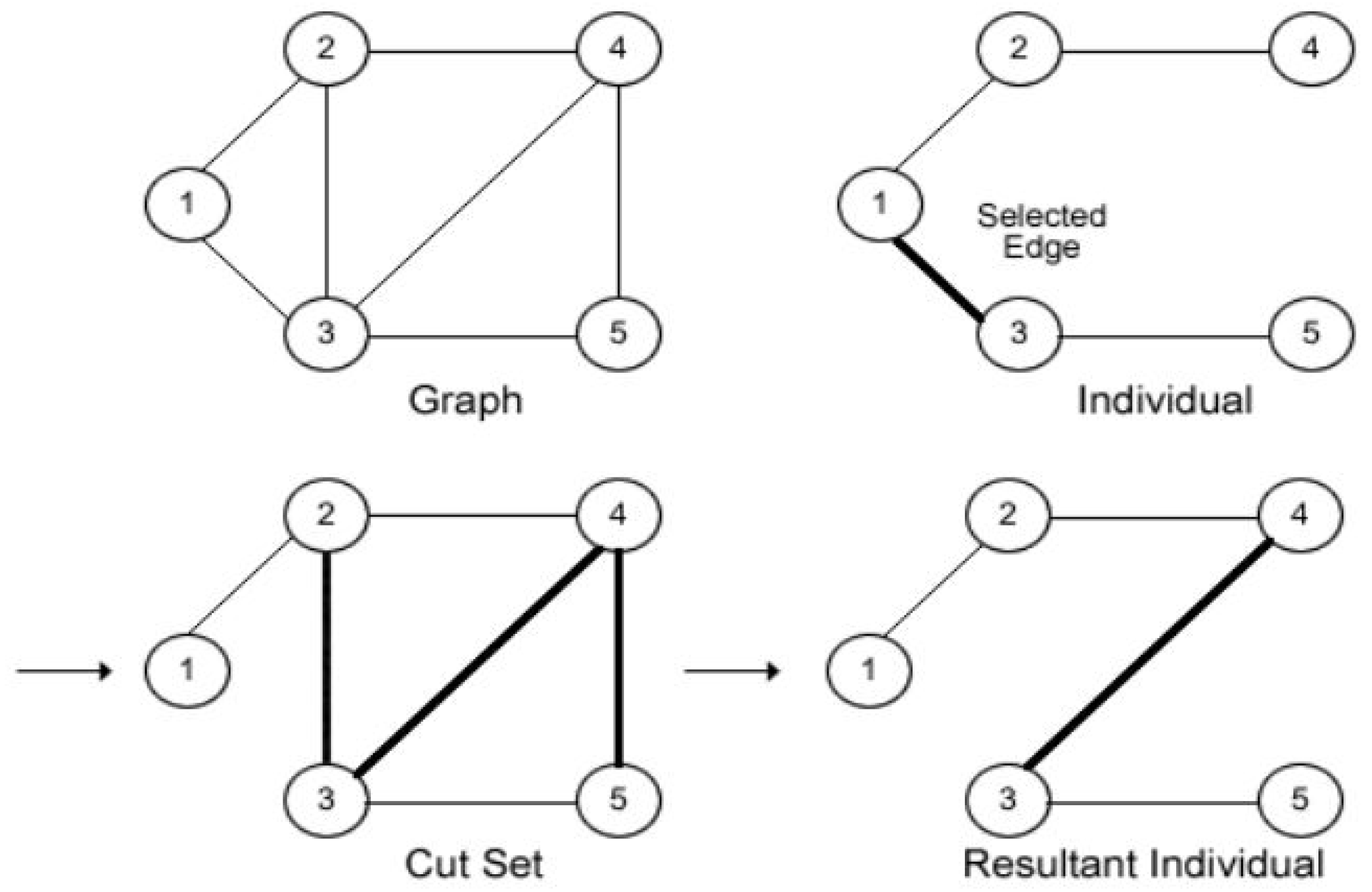
The mutation process is achieved by randomly selecting an edge ${\mathsf{e}}_{\mathsf{i},\mathsf{j}}$ from a chosen MST $\mathsf{T}\mathsf{3}$ contained in the population and removing ${\mathsf{e}}_{\mathsf{i},\mathsf{j}}$ from $\mathsf{T}\mathsf{3}$ and the original network graph $\mathsf{G}$ to create the sub-graphs $\mathsf{G}\mathsf{2}$ and ${\mathsf{G}}^{\ast }$, respectively. A random edge ${\mathsf{e}}_{\mathsf{i},\mathsf{j}}^{\ast }$ contained in the cut set of ${\mathsf{G}}^{\ast }$ is added to $\mathsf{G}\mathsf{2}$ to form a new sub-graph, $\mathsf{G}{\mathsf{2}}^{\ast }$ [51].

The cut set of ${\mathsf{G}}^{\ast }$ is the set of edges contained in ${\mathsf{G}}^{\ast }$ and are not contained in $\mathsf{G}\mathsf{2}$. The individual formed by the mutation process has to be a tree of $\mathsf{G}$ before it is accepted, as illustrated in Figure 2. The number of times to apply the mutation operator before choosing the fitness individual is specified by the mutation rate $mr$.

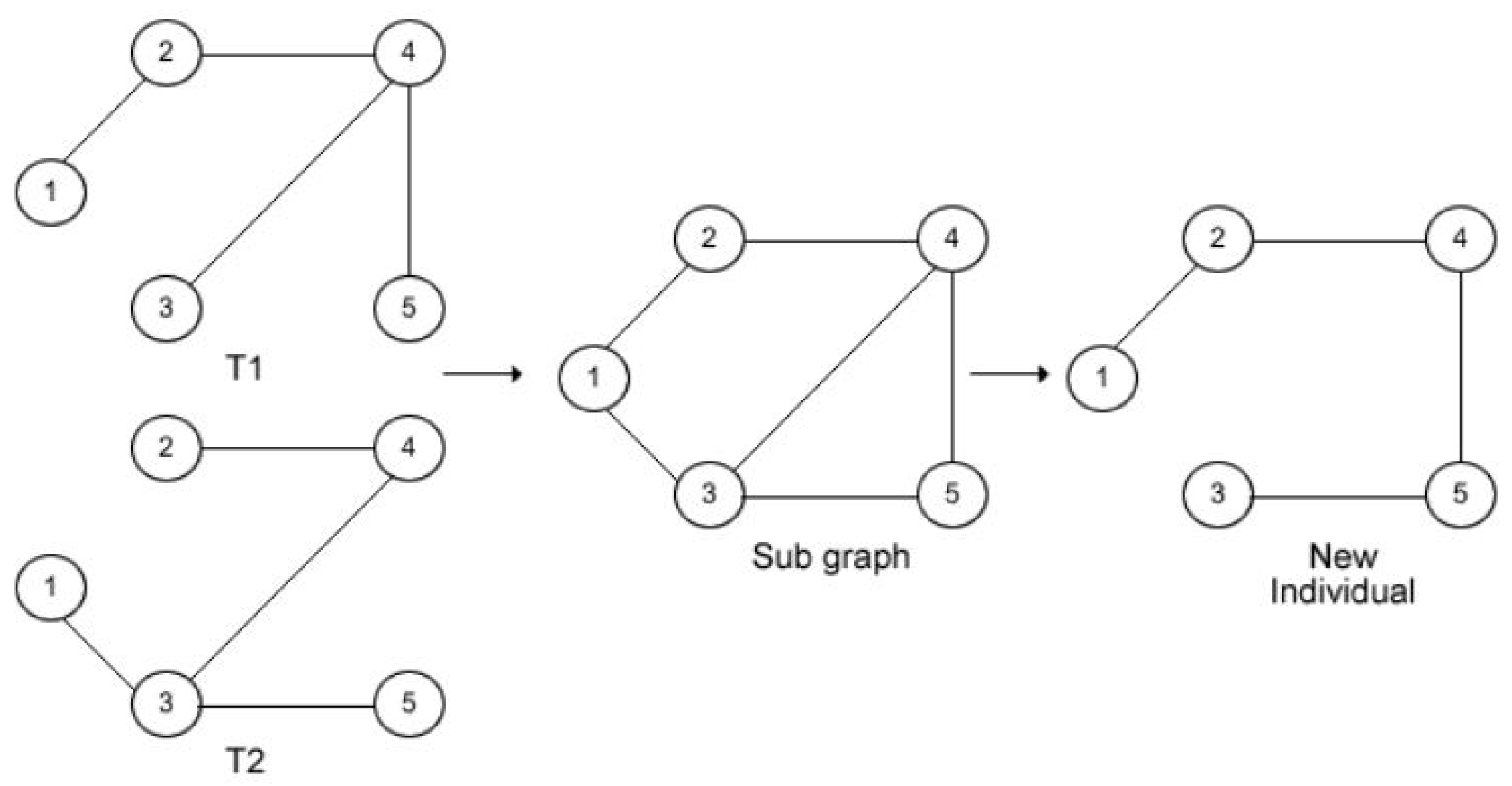
The crossover process is achieved by selecting two individuals $\mathsf{T}\mathsf{1}$ and $\mathsf{T}\mathsf{2}$ randomly from the population as parents to create offspring for the subsequent generation. $\mathsf{T}\mathsf{1}$ and $\mathsf{T}\mathsf{2}$ are joined to create a sub-graph $\mathsf{G}\mathsf{1}$ of $\mathsf{G}$ by passing the union operation [51]. The individual form is an MST of $\mathsf{G}\mathsf{1}$ and the network graph $\mathsf{G}$ as shown in Figure 3. The number of times the crossover operator is carried out is determined by the crossover rate $cr$.

3.2. A Centralized Routing Protocol for Lifetime and Energy Optimization Using GA and LSPI

After the network initialization, the sink generates possible distance-based MSTs using the GA-based MSTs. The generated MSTs are used as the routing tables (RTs) by the CRPLEOGALSPI. The optimization problem addressed by the CRPLEOGALSPI is to maximize the network lifetime while minimizing the network energy consumption in the WSNs. The optimization problem is formulated as a bi-objective mixed integer programming defining the objective function and the set of constraints.

The optimization problem is to find the RT such that:

$$\begin{array}{c}\hfill \underset{v\in V}{\max }\left\{ESR{E}_v\right\}+\underset{v,u\in V}{\min }\left\{\sum _{u=0}^{\left|V\right|}\sum _{v=0}^{\left|V\right|}{e}_{u,v}E{C}_{u,v}\right\}subjectto\end{array}$$

(22a)

$$\begin{array}{c}\hfill \sum _{u=0,u\ne v}^{\left|V\right|}{e}_{u,v}=1\end{array}$$

(22b)

$$\begin{array}{c}\hfill \sum _{v=0,u\ne v}^{\left|V\right|}{e}_{u,v}=1\end{array}$$

(22c)

$$\begin{array}{c}\hfill d_{u,v}\le R_{max}\end{array}$$

(22d)

$$\begin{array}{c}\hfill e_{u,v}\in \{0,1\}\end{array}$$

(22e)

Equation (22a) is the objective function and Equations (22b)–(22e) are the constraints. The variable $ESR{V}_v$ is the estimated sensor node residual energy of the vth sensor node. $e_{u,v}$ is the connection index when the uth sensor node is connected to the vth sensor node. $E_{u,v}$ is the energy consumption when the uth sensor node communicates with the vth sensor node. $d_{u,v}$ is the link distance between the uth sensor node and the vth sensor node. $R_{max}$ is the network’s maximum transmission radius.

The first term of the objective function in Equation (22a) is used to maximize the network lifetime, while the second term is used to minimize the network energy consumption. The constraints in Equation (22b) and (22c) ensure that the routing path is a tree. The constraint in Equation (22d) enables transmission between two connected sensor nodes whose link distance is less than or equal to the maximum network transmission radius.

Therefore, the CRPLEOGALSPI tries to find the RT that maximizes the network lifetime while minimizing the network energy consumption using LSPI. The network lifetime considered in the design of the CRPLEOGALSPI is the time for the network graph to be disconnected; that is, the time taken for an alive sensor node not to find a path to the sink for data transmission. The CRPLEOGALSPI is deployed at the sink.

The solving process of the objective function subject to the constraints is given in the design of the proposed protocol using LSPI and is provided in the sequel.

The state space and action space of the agent are the MSTs generated by the GA-based MSTs. For a current MST, s, being used by the sink in receiving data from the sensor nodes, the action of the agent is to choose another MST, a, that maximizes the network lifetime while minimizing the network energy consumption. The next state of the agent, $\widehat{s}$ is the same as the choosing action in the current learning episode, that is, $P\left(\widehat{s}\right|s,a)=1$. The features considered in designing the basic functions of the CRPLEOGALSPI for the state–action pair are the maximum energy consumption of the sensor nodes, $E{C}_{max}(s,a)$ and the sum of the energy consumption of the sensor nodes, $E{C}_{sum}(s,a)$ when using a to receive data packets by the sink.

The first basic function is used to model the maximization of the network lifetime, while the second basic function is used to model the minimization of the network energy consumption. The set of the basic functions for the state–action pair $(s,a)$ is therefore given as $\phi (s,a)=\left\{E{C}_{max}(s,a),E{C}_{sum}(s,a)\right\}$.

The Q-values of the state–action pair are approximated using Equation (23)

$$\widehat{Q}(s,a)=w_{1}E{C}_{max}(s,a)+w_{2}E{C}_{sum}(s,a)=w\phi {(s,a)}^T$$

(23)

where $w_1$ and $w_2$ are the weights associated to the basic functions $E{C}_{max}(s,a)$ and $E{C}_{sum}(s,a)$, respectively, w is the weight matrix of size $2\times 1$ and $\phi {(s,a)}^T$ is the transpose of the basic function matrix of size $1\times 2$.

The weight, w in the Equation (23) is approximated using a set of samples $\mathcal{D}=\left\{(s_i,a_i,r_i,\widehat{s_i})|i=1,2\dots ,M\right\}$ as given in Equation (24).

$$\widehat{w}={\widehat{X}}^{-1}\widehat{y}$$

(24)

The set of samples $\mathcal{D}$ is obtained by taking a random action in a given state.

The algorithm used to generate the random samples by the sink is given in Algorithm 3.

Algorithm 3 Samples Generation Algorithm.

Input:  List of RTs, Maximum number of samples, ${\left|\mathcal{D}\right|}_{max}$, Number of iterations, N Output:  Set of samples, $\mathcal{D}$ 1: $\mathcal{D}=\left\{\right\}$ 2: Initialize a random RT as $s_0$ 3: for$i=1$ to N do 4:    $s_i=s_o$ 5:    The agent Choose a random RT, $a_i$ 6:    The agent receives a reward, $r_i$ using Equation (27) 7:    $s_i\leftarrow s_o$ 8:    $\widehat{s_i}=s_o$ 9:    if $(s_i,a_i,\widehat{s_i},r_i)\notin \mathcal{D}$ then 10:      $\mathcal{D}\leftarrow (s_i,a_i,\widehat{s_i},r_i)$ 11:    end if 12:    if $\left|\mathcal{D}\right|={\left|\mathcal{D}\right|}_{max}$ then 13:      break 14:    end if 15: end for 16: Return $\mathcal{D}$

Assuming ${\widehat{X}}^0=0$ and ${\widehat{y}}^0=0$ initially, Equations (25) and (26) will give the approximated values of ${\widehat{X}}^{i+1}$ and ${\widehat{y}}^{i+1}$, respectively, of a new sample $(s_i,a_i,r_i,\widehat{s_i})$

$${\widehat{X}}^{i+1}\leftarrow {\widehat{X}}^i+\phi (s_i,a_i){\left[\phi (s_i,a_i)-\gamma \phi (\widehat{s_i},\underset{a\in A}{\mathrm{argmin}}(\widehat{s_i},a))\right]}^T$$

(25)

where $\gamma$ is the discount factor.

$${\widehat{y}}^{i+1}\leftarrow {\widehat{y}}^i+\phi (s_i,a_i)r_i$$

(26)

The reward obtained is modeled as in Equation (27)

$$r_i=\underset{v\in V}{\max }\left\{E{C}_v\right\}+\underset{v\in V}{\mathrm{sum}}\left\{E{C}_v\right\}$$

(27)

where $E{C}_v$ is the energy consumption by the vth sensor node.

The sink evaluates the $E{C}_v$ after each learning round using the difference between the formerly estimated sensor residual energy $ESR{E}_v^{Previous}$ and the later estimated sensor residual energy, $ESR{E}_v^{Current}$. Therefore $E{C}_v$ is as given in Equation (28).

$$E{C}_v=ESR{E}_v^{Former}-ESR{E}_v^{Later}$$

(28)

The network lifetime is maximized while minimizing the energy consumption of the WSN by learning the RT that minimizes the Q-value using the epsilon-greedy technique. Given a number, $z\in (0,1)$ randomly generated in each learning round and a probability epsilon value, $ϵ\in [0,1]$, the agent selects its action in each learning round with the policy given in Equation (29).

$$a_t=\left\{\begin{array}{c}\underset{a}{\mathrm{argmin}}\left(\phi {(s,a)}^{T}w\right),ifz<1-ϵ\hfill \\ Randomaction,otherwise.\hfill \end{array}\right.$$

(29)

The designed CRPLEOGALSPI for learning the optimal RT to maximize network lifetime and minimize the network energy consumption is given in Algorithm 4. The novelty of the proposed protocol is in the use of the LSPI, which tends to converge faster to the best RT in solving the objective function subject to constraints when compared to Q-learning.

Algorithm 4 CRPLEOGALSPI.

Input:  $\mathsf{G}(\mathsf{V},\mathsf{E})$, Basic Functions, $\phi$, $\gamma$, $ϵ$, Learning round (L), stopping criterion, $\epsilon$ Output:  Optimal RT(s) 1: Sink executes Algorithm 2 to generate List of RTs 2: Sink collect set of samples, $\mathcal{D}$ with Algorithm 3 3: Initialize $s_0$ as a random RT 4: Initialize ${\widehat{X}}^0\leftarrow 0$ and ${\widehat{y}}^0\leftarrow 0$ 5: Initialize weight, $w_o\leftarrow 0$ 6: $\widehat{w}\leftarrow w_o$ 7: repeat 8:    $w\leftarrow \widehat{w}$ 9:    for $(s_i,a_i,r_i,\widehat{s_i})\in \mathcal{D}$ do 10:      ${\widehat{X}}^{i+1}\leftarrow {\widehat{X}}^i+\phi (s_i,a_i){\left[\phi (s_i,a_i)-\gamma \phi (\widehat{s_i},\underset{a\in A}{\mathrm{argmin}}(\widehat{s_i},a))\right]}^T$ 11:      ${\widehat{y}}^{i+1}\leftarrow {\widehat{y}}^i+\phi (s_i,a_i)r_i$ 12:    end for 13:     $\widehat{w}={\widehat{X}}^{-1}\widehat{y}$ 14: until$\left|\right|w-\widehat{w}\left|\right|<\epsilon$ 15: returnw 16: for$t=1$ to L do 17:    $s_t=s_o$ 18:    Sink chooses an RT using Equation (29) 19:    Sink receives data from the sensors using the chosen RT. 20:    Updates $s_o$ as the current RT. 21:    if Any sensor node dies, then 22:      Delete the dead sensor node(s) from $G(V,E)$ 23:      Delete edges connected to the dead sensor node(s) 24:      Rebuild $\mathsf{G}(\mathsf{V},\mathsf{E})$ 25:      if $\mathsf{G}(\mathsf{V},\mathsf{E})$ is connected, then 26:         Do steps 1 to 20 27:      else 28:         $break$ 29:      end if 30:    end if 31: end for

3.3. Energy Consumption Model

The energy consumed by the vth sensor node, $E{C}_v$ in a round of data transmission is the summation of the energy consumed by the sensor node in sending and receiving data packets and is given in the Equation (30).

$$E{C}_v(p,d)=E_{tx}(p,d)+E_{rx}\left(p\right)$$

(30)

The energy consumed by a sensor node for sending and receiving data packets is given in Equations (31) and (33), respectively [33].

$$E_{tx}(p,d)=\left\{\begin{array}{c}{E}_{elec}p\ell +E_{fs}p{d}^{2}ifd⩽d_o\hfill \\ elecp\ell +E_{mp}p{d}^{4}ifd>d_o\hfill \end{array}\right.$$

(31)

$$E_{rx}\left(p\right)=E_{elec}p\tau$$

(32)

where p is the number of bits per packet, d is the distance between the source node and the destination node, ℓ is the number of packets sent by a sensor node per round, $\tau$ is the number of packets received by a sensor node per round, $E_{tx}(p,d)$ is the transmission energy, $E_{rx}\left(p\right)$ is the reception energy, and $E_{elec}$ is the electronic energy consumed to transmit or receive unit data of the packet. $E_{fs}$, $E_{mp}$ are the transmit amplifier efficiency and depend on the transmitter amplifier model (free space model is employed when $d⩽d_o$, otherwise the multipath model is employed). $d_o$ is the baseline distance and is obtained by equating the two expressions of $E_{tx}(p,d)$ at $d=d_o$ and is given as:

$$d_o=\sqrt{\frac{E_{fs}}{E_{mp}}}$$

(33)

4. Simulation and Results Discussion

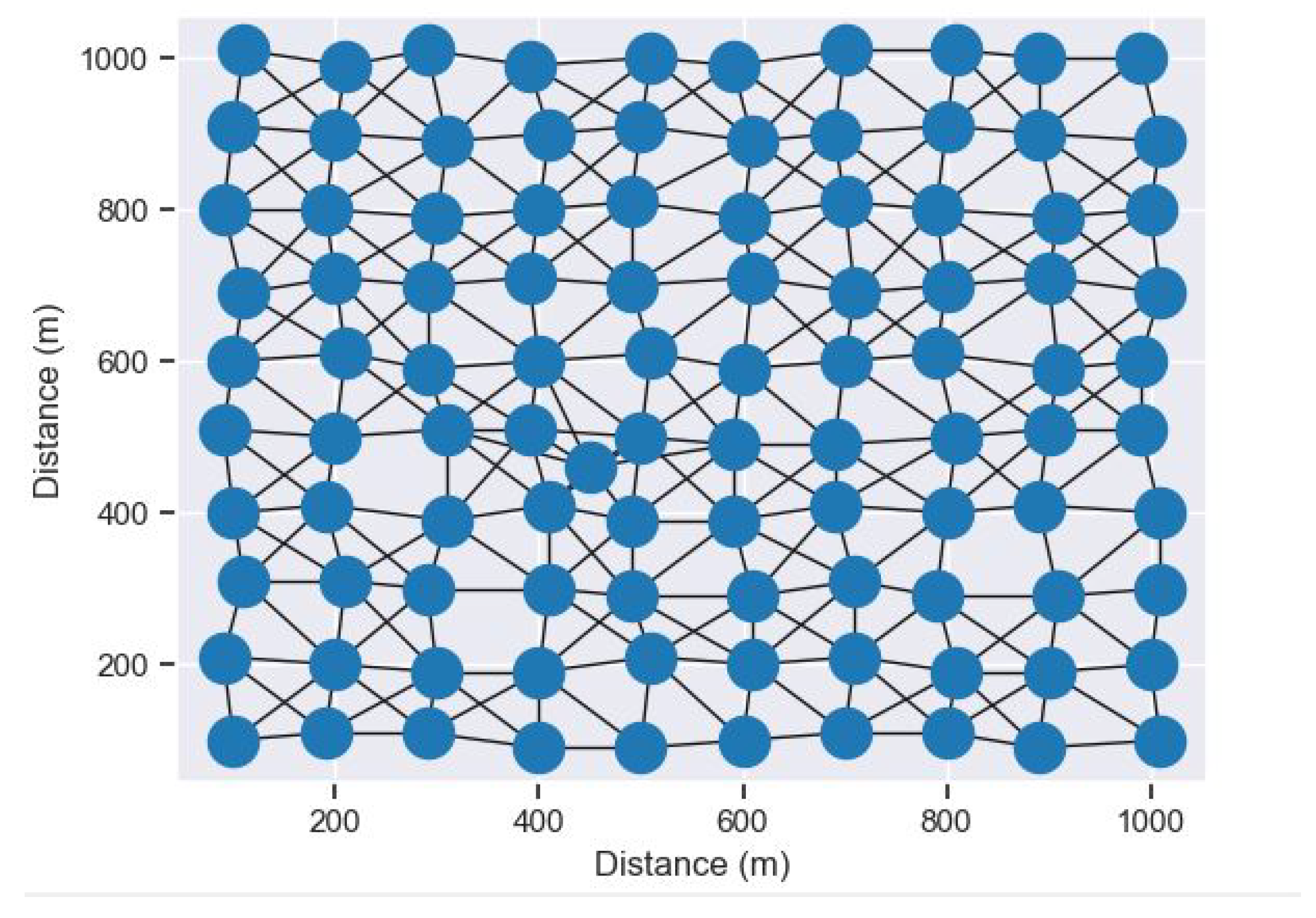
The performance of the GA-based MSTs is first established for convergence using simulation. Secondly, the performance analysis of the proposed routing protocol is achieved with simulations using the performance metrics of network lifetime, number of alive sensor nodes (NAN), energy consumption, and computation time. These performance metrics of the CRPLEOGALSPI are compared with that of the recent CRPLOGARL [13] as a way of validation. The lifetime of the network is calculated as the time taken for the sink not to be reachable by the alive sensor node(s). The NAN is the number of alive sensor nodes at the lifetime of the network. The CRPLEOGALSPI and CRPLOGARL are coded with python 3.8 under the “PyCharm” development environment. The graphical layout of the WSN is implemented with the python NetworkX module [52]. The python codes are executed on the SLURM (Simple Linux Utility for Resource Management) cluster on the IRIT’s OSIRIM platform. The Computer nodes of the OSIRIM platform adopted are the 4 AMD EPYC 7402 bi-processor computing nodes at 2.8 GHz, with 48 processors and 512 GB of RAM each. These nodes enable more than 24 threads and/or 192 GB of RAM for the same process. The simulation parameters used to carry out the performance analysis and the network graph of the deployed WSN are shown in

Table 2. Simulation Parameters.

Parameters	Values
Number of sink	1
Number of sensors	100
Deployment Area of WSN	1000 m × 1000 m
Deployment of Sensor nodes	Random
$x-y$ coordinate of sink	$(500,500)$
Maximum transmission range	150 m
Bandwidth of links	1 kbps
Size of data packet	1024 bits
Sensors initial residual energy	1 J to 10 J
Rate of packet generation	1/s to 10/s
$e_{mp}$	0.0013 pJ/bit/m${}^4$
$e_{fs}$	10 pJ/bit/m${}^2$
$E_{elec}$	50 nJ/bit
Discount factor	0.9
Epsilon	0.1
Sample size	100
Maximum generations	1000
Rate of crossover	0.1
Rate of Mutation	1

and Figure 4, respectively.

The performance of the GA-based MSTs for the deployed network graph of the WSN given in Figure 4 is shown in Figure 5.

As seen in Figure 5, the GA-based MSTs is able to find 376 MSTs of the network graph for 1000 generations. This also implies the convergence of the solution of the GA-based MSTs in a reasonable number of generations. The GA-based MSTs can work for all MSTs problems in polynomial time.

The number of alive sensor nodes of the WSN at each round of data transmission of the proposed routing protocol, CRPLEOGALSPI, as compared with CRPLOGARL when the initial sensor nodes energies and the packet generation rate of the sensor nodes are set arbitrarily at 10 J and 1/s, respectively, as shown in Figure 6. As seen in Figure 6, the number of alive sensor nodes of both protocols remains constant for certain rounds of data transmission and decreases subsequently. This behavior continues for both protocols until the network graph is disconnected. When the network graph is disconnected, there is no path to reach the sink located at the $x-y$ coordinates of $(500,500)$, as shown in Figure 4. The deaths of the sensor nodes are because of the depletion of the energy of the sensor nodes as the round of data transmission increases. Consequently, on average, it took CRPLEOGALSPI more rounds of data transmission for the sink not to be reachable by alive sensor nodes. This is because CRPLEOGALSPI converges faster to the RT, which maximizes the network lifetime while minimizing the network energy consumption when compared to CRPLOGARL. This shows that the LSPI used in implementing CRPLEOGALSPI utilizes data effectively and efficiently when compared to the baseline Q-learning used to implement the CRPLOGARL.

The time for the sink not to be reachable by the alive sensor nodes of the CRPLEOGALSPI is compared with the CRPLOGARL for increasing sensor nodes’ initial energy as shown in Figure 7. The network lifetime increases with the increase in the initial sensor node energy. This is because the lifetime of a sensor node is proportional to the residual energy of the sensor node.

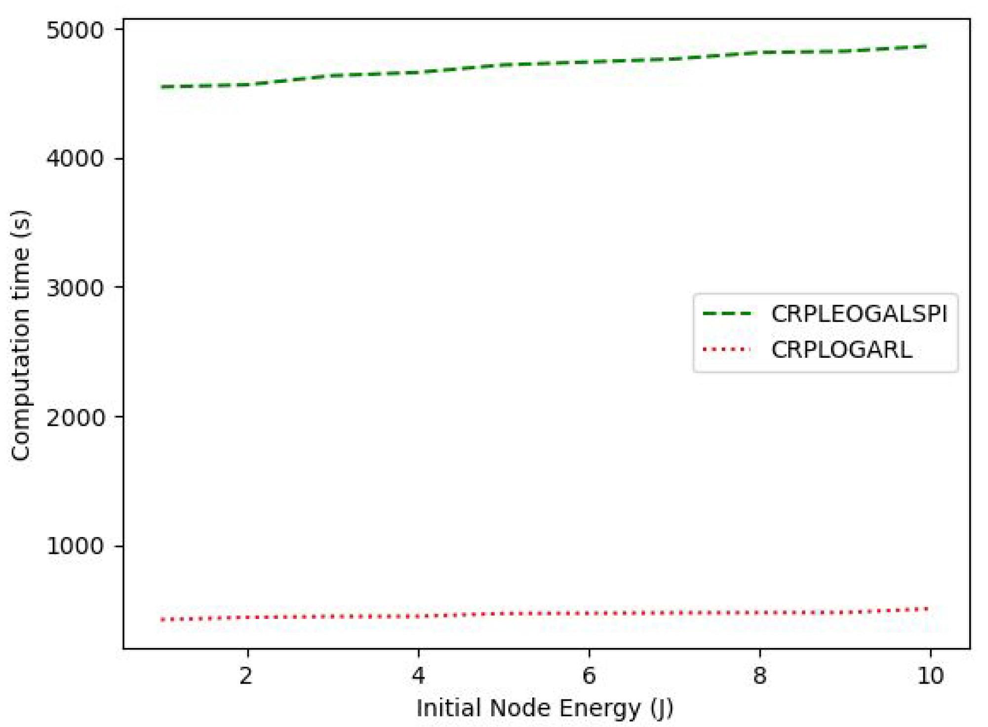
The proposed CRPLEOGALSPI has an improved network lifetime performance of 18.04% when compared to the CRPLOGARL with increasing sensor node residual energy. This is because the CRPLEOGALSPI utilizes LSPI, which is more data efficient and converges faster to the RT, which balances the energy consumption among the sensor nodes and minimizes the network energy consumption as shown in Figure 8. This is against the CRPLOGARL that utilizes the baseline Q-learning that takes larger episodes to converge to the RT that optimizes the network lifetime due to the many RTs. The network energy consumption for both protocols increases with the increase of the initial energy of the sensor nodes. This is because the more the initial sensor nodes’ energy, the more rounds of data transmission it takes for the sensor nodes to deplete their energy. Subsequently, the CRPLEOGALSPI has a reduced energy consumption of 58.96% when compared to CRPLOGARL for increasing the initial energy of the sensor nodes. This is because CRPLEOGALSPI optimizes the network lifetime and the network energy consumption using LSPI. This is against the CRPLOGARL, which optimizes only the network lifetime using Q-learning. This also implies that CRPLEOGALSPI has a reduced $C{O}_2$ footprint when compared to CRPLOGARL for increased initial sensor node energy. This is because $C{O}_2$ footprint is directly proportional to the network energy consumption. However, the improved performance in the network lifetime and network energy consumption of the proposed protocol comes with an increased computation time of about ten times when compared to CRPLOGARL for an increased initial sensor node energy, as shown in Figure 9. This is because CRPLEOGALSPI requires the collection of samples to learn the optimal path each time the network is rebuilt because of the death of sensor node(s).

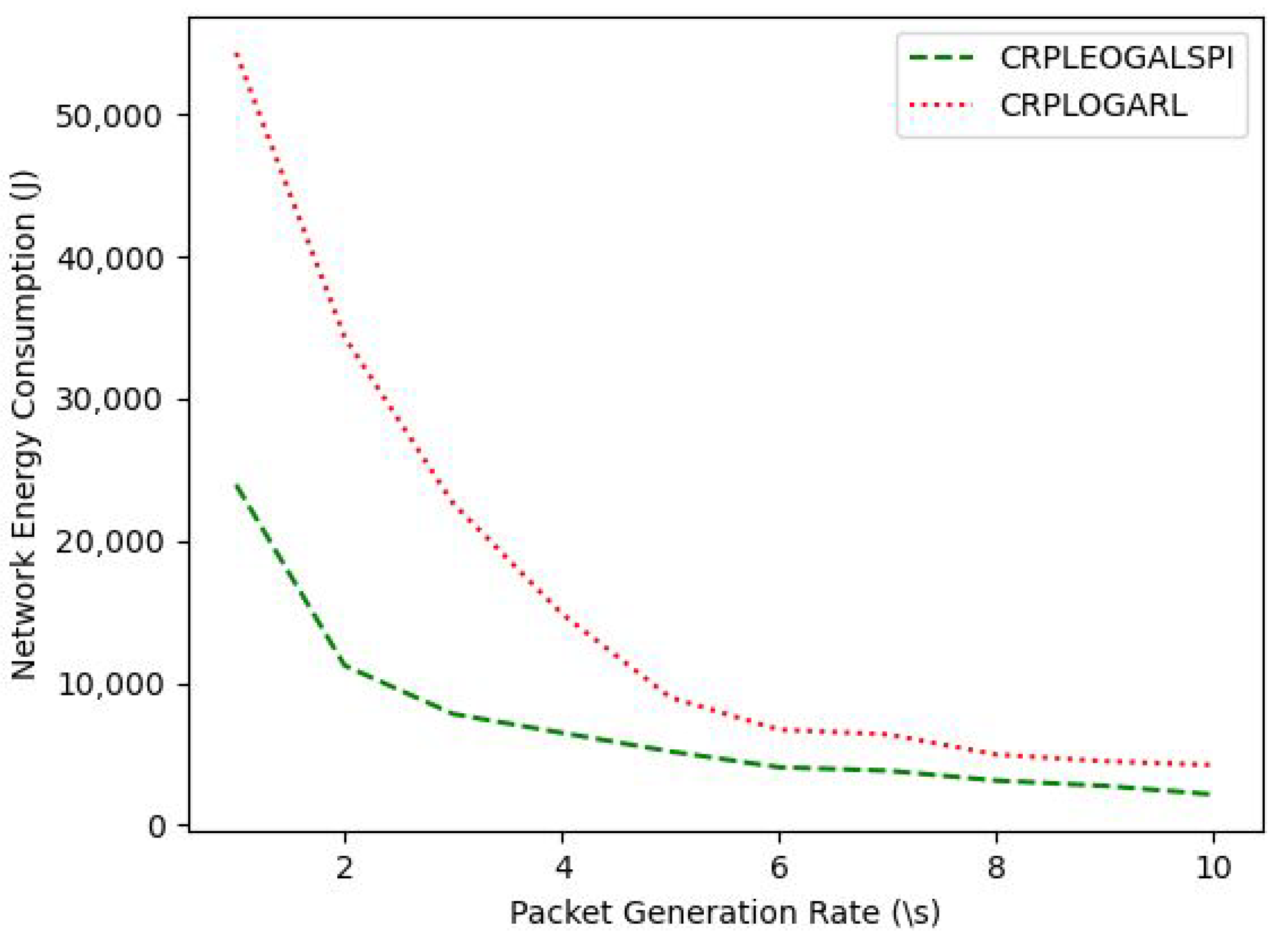
The time for the sink not to be reachable by alive sensor nodes of the CRPLEOGALSPI is compared with the CRPLOGARL for increasing sensor nodes’ packet generation rate as shown in Figure 10. The network lifetime decreases with the increased packet generation rate of the sensor nodes. This is because the network lifetime of a sensor node is inversely proportional to the number of packets transmitted by the sensor node. The proposed CRPLEOGALSPI has an improved network lifetime performance of 14.91% when compared to CRPLOGARL with an increasing packet generation rate of the sensor nodes.

This is because CRPLEOGALSPI utilizes LSPI, which is more data efficient and converges faster to the RT, which balances the energy consumption among the sensor nodes and minimizes the network energy consumption, as shown in Figure 11. This is against the CRPLOGARL that utilizes the baseline Q-learning that takes larger episodes to converge to the RT that optimizes the network lifetime due to the many RTs. The network energy consumption for both protocols decreases with the increasing packet generation rate of the sensor nodes. This is because the more the number of data packets generated and transmitted by the sensor nodes, the fewer rounds of data transmission it takes for the sensor nodes to deplete their energy. Subsequently, the CRPLEOGALSPI has a reduced energy consumption of 56.36% when compared to the CRPLOGARL for increasing the packet generation rate of the sensor nodes. This is because the CRPLEOGALSPI optimizes the network lifetime and the network energy consumption using LSPI. This is contrasted with the CRPLOGARL, which optimizes only the network lifetime using Q-learning. This also implies that the CRPLEOGALSPI has a reduced $C{O}_2$ footprint when compared to the CRPLOGARL for an increased sensor node packet generation rate. This is because that $C{O}_2$ footprint is directly proportional to the network energy consumption.

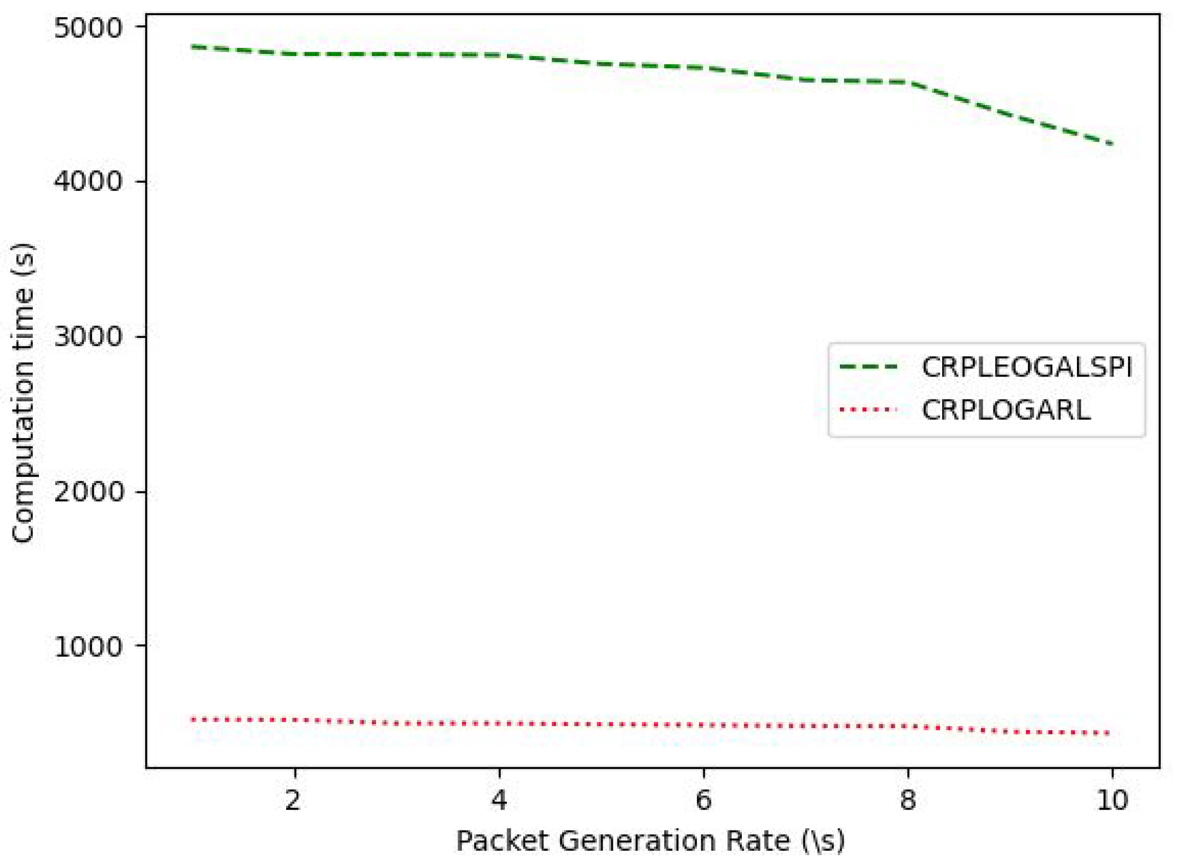
But, the improved performance in the network lifetime and network energy consumption of the proposed protocol comes with an increased computation time of about ten times that of the CRPLOGARL for an increased packet generation rate of the sensor node, as shown in Figure 12. This is because the CRPLEOGALSPI requires the collection of samples and iteration over the collected samples to learn the optimal policy each time the network is rebuilt because of the death of sensor node(s).

5. Conclusions

This paper presented the design of a centralized routing protocol for lifetime and energy optimization using a GA and LSPI for WSNs. The sink generates the routing tables of the network graph in polynomial time using a GA. The LSPI deployed at the sink learns the optimal routing path for lifetime and energy optimization at each stage of the network graph, building after the death of sensor nodes. This leads to the maximization of the time taken for the sink not to be reachable by the alive sensor nodes while minimizing the network energy consumption. The centralized routing protocol for lifetime and energy optimization using a GA and LSPI improves network lifetime and energy consumption when compared with the existing Centralized Routing Protocol for Lifetime Optimization using Genetic Algorithm and Q-learning. This is because the centralized routing protocol for lifetime and energy optimization using GA and LSPI converges faster to the optimal routing path and is not sensitive to parameter settings. However, the improved performance in the network lifetime and network energy consumption of the proposed protocol comes with an increased computation time. Future work will consider emulating the proposed protocol using Mininet, considering the real-world parameters of a typical WSN, and taking into consideration the cost of control packets and prioritization schemes when some sensor nodes send more data packets than others.

References

1. Priyadarshi, R.; Gupta, B.; Anurag, A. Deployment techniques in wireless sensor networks: A survey, classification, challenges, and future research issues. J. Supercomput. 2020, 76, 7333–7373. [Google Scholar] [CrossRef]
2. Rawat, P.; Singh, K.D.; Chaouchi, H.; Bonnin, J.M. Wireless sensor networks: A survey on recent developments and potential synergies. J. Supercomput. 2014, 68, 1–48. [Google Scholar] [CrossRef]
3. Matin, M.A.; Islam, M.M. Overview of wireless sensor network. Wirel. Sens. Netw.-Technol. Protoc. 2012, 1, 1–24. [Google Scholar]
4. Xia, F. Wireless sensor technologies and applications. Sensors 2009, 9, 8824–8830. [Google Scholar] [CrossRef] [PubMed] [Green Version]
5. Engmann, F.; Katsriku, F.A.; Abdulai, J.D.; Adu-Manu, K.S.; Banaseka, F.K. Prolonging the lifetime of wireless sensor networks: A review of current techniques. Wirel. Commun. Mob. Comput. 2018, 1–23. [Google Scholar] [CrossRef] [Green Version]
6. Nayak, P.; Swetha, G.K.; Gupta, S.; Madhavi, K. Routing in wireless sensor networks using machine learning techniques: Challenges and opportunities. Measurement 2021, 178, 1–15. [Google Scholar] [CrossRef]
7. Al Aghbari, Z.; Khedr, A.M.; Osamy, W.; Arif, I.; Agrawal, D.P. Routing in wireless sensor networks using optimization techniques: A survey. Wirel. Pers. Commun. 2020, 111, 2407–2434. [Google Scholar] [CrossRef]
8. Mostafaei, H.; Menth, M. Software-defined wireless sensor networks: A survey. J. Netw. Comput. Appl. 2018, 119, 42–56. [Google Scholar] [CrossRef]
9. Obi, E.; Mammeri, Z.; Ochia, O.E. A Lifetime-Aware Centralized Routing Protocol for Wireless Sensor Networks using Reinforcement Learning. In Proceedings of the 17th International Conference on Wireless and Mobile Computing, Networking and Communications, Bologna, Italy, 11–13 October 2021; pp. 363–368. [Google Scholar]
10. Sutton, R.S.; Barto, A.G. Reinforcement Learning: An Introduction, 2nd ed.; MIT press: Cambridge, MA, USA; London, UK, 2018; pp. 119–138. [Google Scholar]
11. Yamada, T.; Kataoka, S.; Watanabe, K. Listing all the minimum spanning trees in an undirected graph. Int. J. Comput. Math. 2010, 87, 3175–3185. [Google Scholar] [CrossRef]
12. Whitley, D. A genetic algorithm tutorial. Stat. Comput. 1994, 4, 65–85. [Google Scholar] [CrossRef]
13. Obi, E.; Mammeri, Z.; Ochia, O.E. Centralized Routing for Lifetime Optimization Using Genetic Algorithm and Reinforcement Learning for WSNs. In Proceedings of the 16th International Conference on Sensor Technologies and Applications, Lisbon, Portugal, 16–20 October 2022; pp. 5–12. [Google Scholar]
14. Watkins, C.J.; Dayan, P. Q-learning. Mach. Learn. 1992, 8, 279–292. [Google Scholar] [CrossRef]
15. Lagoudakis, M.G.; Parr, R. Least-squares policy iteration. J. Mach. Learn. Res. 2003, 4, 1107–1149. [Google Scholar]
16. Kaelbling, L.P.; Littman, M.L.; Moore, A.W. Reinforcement learning: A survey. J. Artif. Intell. Res. 1996, 4, 237–285. [Google Scholar] [CrossRef] [Green Version]
17. Mammeri, Z. Reinforcement learning based routing in networks: Review and classification of approaches. IEEE Access 2019, 7, 55916–55950. [Google Scholar] [CrossRef]
18. Bradtke, S.J.; Barto, A.G. Linear least-squares algorithms for temporal difference learning. Mach. Learn. 1996, 22, 33–57. [Google Scholar] [CrossRef] [Green Version]
19. Boyan, J.; Littman, M. Packet routing in dynamically changing networks: A reinforcement learning approach. Adv. Neural Inf. Process. Syst. 1993, 6, 671–678. [Google Scholar]
20. Zhang, Y.; Fromherz, M. Constrained flooding: A robust and efficient routing framework for wireless sensor networks. In Proceedings of the 20th International Conference on Advanced Information Networking and Applications-Volume 1, Vienna, Austria, 18–20 April 2006; pp. 1–6. [Google Scholar]
21. Maroti, M. Directed flood-routing framework for wireless sensor networks. In Proceedings of the ACM/IFIP/USENIX International Conference on Distributed Systems Platforms and Open Distributed Processing, Berlin, Germany, 18–20 October 2004; pp. 99–114. [Google Scholar]
22. He, T.; Krishnamurthy, S.; Stankovic, J.A.; Abdelzaher, T.; Luo, L.; Stoleru, R.; Yan, T.; Gu, L.; Hui, J.; Krogh, B. Energy-efficient surveillance system using wireless sensor networks. In Proceedings of the 2nd International Conference on Mobile Systems, Applications, and Services, Boston, MA, USA, 6–9 June 2004; pp. 270–283. [Google Scholar]
23. Intanagonwiwat, C.; Govindan, R.; Estrin, D. Directed diffusion: A scalable and robust communication paradigm for sensor networks. In Proceedings of the 6th Annual International Conference on Mobile Computing and Networking, Boston, MA, USA, 6–11 August 2000; pp. 56–67. [Google Scholar]
24. Wang, P.; Wang, T. Adaptive routing for sensor networks using reinforcement learning. In Proceedings of the 6th IEEE International Conference on Computer and Information Technology, Seoul, Republic of Korea, 20–22 September 2006; p. 219. [Google Scholar]
25. Nurmi, P. Reinforcement learning for routing in ad hoc networks. In Proceedings of the 5th IEEE International Symposium on Modeling and Optimization in Mobile, Ad Hoc and Wireless Networks and Workshops, Limassol, Cyprus, 16–20 April 2007; pp. 1–8. [Google Scholar]
26. Dong, S.; Agrawal, P.; Sivalingam, K. Reinforcement learning based geographic routing protocol for UWB wireless sensor network. In Proceedings of the IEEE Global Telecommunications Conference, Washington, DC, USA, 26–30 November 2007; pp. 652–656. [Google Scholar]
27. Karp, B.; Kung, H.T. GPSR: Greedy perimeter stateless routing for wireless networks. In Proceedings of the 6th Annual International Conference on Mobile Computing and Networking, Boston MA, USA, 6–11 August 2000; pp. 243–254. [Google Scholar]
28. Arroyo-Valles, R.; Alaiz-Rodriguez, R.; Guerrero-Curieses, A.; Cid-Sueiro, J. Q-probabilistic routing in wireless sensor networks. In Proceedings of the IEEE 3rd International Conference on Intelligent Sensors, Sensor Networks and Information, Melbourne, VIC, Australia, 3–6 December 2007; pp. 1–6. [Google Scholar]
29. Naruephiphat, W.; Usaha, W. Balancing tradeoffs for energy-efficient routing in MANETs based on reinforcement learning. In Proceedings of the VTC Spring IEEE Vehicular Technology Conference, Marina Bay, Singapore, 11–14 May 2008; pp. 2361–2365. [Google Scholar]
30. Förster, A.; Murphy, A.L. Balancing energy expenditure in WSNs through reinforcement learning: A study. In Proceedings of the 1st International Workshop on Energy in Wireless Sensor Networks, Santorini Island, Greece, 11–14 June 2008; pp. 1–7. [Google Scholar]
31. Hu, T.; Fei, Y. QELAR: A q-learning-based energy-efficient and lifetime-aware routing protocol for underwater sensor networks. In Proceedings of the IEEE International Performance, Computing and Communications Conference, Austin, TX, USA, 7–9 December 2008; pp. 247–255. [Google Scholar]
32. Yang, J.; Zhang, H.; Pan, C.; Sun, W. Learning-based routing approach for direct interactions between wireless sensor network and moving vehicles. In Proceedings of the 16th International IEEE Conference on Intelligent Transportation Systems, The Hague, The Netherlands, 6–9 October 2013; pp. 1971–1976. [Google Scholar]
33. Oddi, G.; Pietrabissa, A.; Liberati, F. Energy balancing in multi-hop Wireless Sensor Networks: An approach based on reinforcement learning. In Proceedings of the 2014 NASA/ESA IEEE Conference on Adaptive Hardware and Systems, Leicester, UK, 14–17 July 2014; pp. 262–269. [Google Scholar]
34. Jafarzadeh, S.Z.; Moghaddam, M.H.Y. Design of energy-aware QoS routing protocol in wireless sensor networks using reinforcement learning. In Proceedings of the 2014 IEEE 27th Canadian Conference on Electrical and Computer Engineering, Toronto, ON, Canada, 4–7 May 2014; pp. 1–5. [Google Scholar]
35. Guo, W.J.; Yan, C.R.; Gan, Y.L.; Lu, T. An intelligent routing algorithm in wireless sensor networks based on reinforcement learning. Appl. Mech. Mater. 2014, 678, 487–493. [Google Scholar] [CrossRef]
36. Shah, R.C.; Rabaey, J.M. Energy aware routing for low energy ad hoc sensor networks. In Proceedings of the IEEE Wireless Communications and Networking Conference Record, Orlando, FL, USA, 17–21 March 2002; pp. 350–355. [Google Scholar]
37. Yessad, S.; Tazarart, N.; Bakli, L.; Medjkoune-Bouallouche, L.; Aissani, D. Balanced energy-efficient routing protocol for WSN. In Proceedings of the IEEE International Conference on Communications and Information Technology, Hammamet, Tunisia, 26–28 June 2012; pp. 326–330. [Google Scholar]
38. Debowski, B.; Spachos, P.; Areibi, S. Q-learning enhanced gradient-based routing for balancing energy consumption in WSNs. In Proceedings of the IEEE 21st International Workshop on Computer Aided Modelling and Design of Communication Links and Networks, Toronto, ON, Canada, 23–25 October 2016; pp. 18–23. [Google Scholar]
39. Renold, A.P.; Chandrakala, S. MRL-SCSO: Multi-agent reinforcement learning-based self-configuration and self-optimization protocol for unattended wireless sensor networks. Wirel. Pers. Commun. 2017, 96, 5061–5079. [Google Scholar] [CrossRef]
40. Gnawali, O.; Fonseca, R.; Jamieson, K.; Moss, D.; Levis, P. Collection tree protocol. In Proceedings of the 7th ACM Conference on Embedded Networked Sensor Systems, Berkeley, CA, USA, 4–6 November 2009; pp. 1–14. [Google Scholar]
41. Guo, W.; Yan, C.; Lu, T. Optimizing the lifetime of wireless sensor networks via reinforcement-learning-based routing. Int. J. Distrib. Sens. Netw. 2019, 15, 1–20. [Google Scholar] [CrossRef] [Green Version]
42. Bouzid, S.E.; Serrestou, Y.; Raoof, K.; Omri, M.N. Efficient routing protocol for wireless sensor network based on reinforcement learning. In Proceedings of the 5th IEEE International Conference on Advanced Technologies for Signal and Image Processing, Sousse, Tunisia, 2–5 September 2020; pp. 1–5. [Google Scholar]
43. Sapkota, T.; Sharma, B. Analyzing the energy efficient path in Wireless Sensor Network using Machine Learning. ADBU J. Eng. Technol. 2021, 10, 1–7. [Google Scholar]
44. Intanagonwiwat, C.; Govindan, R.; Estrin, D.; Heidemann, J.; Silva, F. Directed diffusion for wireless sensor networking. IEEE/ACM Trans. Netw. 2003, 11, 2–16. [Google Scholar] [CrossRef] [Green Version]
45. Mutombo, V.K.; Shin, S.Y.; Hong, J. EBR-RL: Energy balancing routing protocol based on reinforcement learning for WSN. In Proceedings of the 36th Annual ACM Symposium on Applied Computing, Virtual Event, 22–26 March 2021; pp. 1915–1920. [Google Scholar]
46. Gibbons, A. Algorithmic Graph Theory; Cambridge University Press: New York, NY, USA, 1985; pp. 121–134. [Google Scholar]
47. Prim, R.C. Shortest connection networks and some generalizations. Bell Syst. Tech. J. 1957, 36, 1389–1401. [Google Scholar] [CrossRef]
48. Kruskal, J.B. On the shortest spanning subtree of a graph and the traveling salesman problem. Proc. Am. Math. Soc. 1956, 7, 48–50. [Google Scholar] [CrossRef]
49. Halim, Z. Optimizing the minimum spanning tree-based extracted clusters using evolution strategy. Clust. Comput. 2018, 21, 377–391. [Google Scholar] [CrossRef]
50. de Almeida, T.A.; Yamakami, A.; Takahashi, M.T. An evolutionary approach to solve minimum spanning tree problem with fuzzy parameters. In Proceedings of the IEEE International Conference on Computational Intelligence for Modelling, Control and Automation and International Conference on Intelligent Agents, Web Technologies and Internet Commerce, Washington, DC, USA, 28–30 November 2005; Volume 2, pp. 203–208. [Google Scholar]
51. Almeida, T.A.; Souza, V.N.; Prado, F.M.S.; Yamakami, A.; Takahashi, M.T. A genetic algorithm to solve minimum spanning tree problem with fuzzy parameters using possibility measure. In Proceedings of the IEEE NAFIPS Annual Meeting of the North American Fuzzy Information Processing Society, Detroit, MI, USA, 26–28 June 2005; pp. 627–632. [Google Scholar]
52. Hagberg, A.; Swart, P.; Daniel, S.C. Exploring network structure, dynamics, and function using NetworkX. In Proceedings of the 8th SCIPY Conference, Pasadena, CA, USA, 19–24 August 2008; pp. 11–15. [Google Scholar]
Figure 1. RL Model as an MDP [10].
Computers 12 00022 g001
Figure 2. MST Mutation.
Computers 12 00022 g002
Figure 3. Crossover between two MSTs T1 and T2.
Computers 12 00022 g003
Figure 4. Network Graph of the deployed WSN.
Computers 12 00022 g004
Figure 5. Number of MSTs with Number of Generations.
Computers 12 00022 g005
Figure 6. Number of alive sensors with Round of Data Transmission.
Computers 12 00022 g006
Figure 7. Network lifetime with Initial Node Energy.
Computers 12 00022 g007
Figure 8. Network Energy Consumption with Initial Node Energy.
Computers 12 00022 g008
Figure 9. Computation time with Initial Node Energy.
Computers 12 00022 g009
Figure 10. Network lifetime with Packet Generation Rate.
Computers 12 00022 g010
Figure 11. Network Energy Consumption with Packet Generation Rate.
Computers 12 00022 g011
Figure 12. Computation time with Packet Generation Rate.
Computers 12 00022 g012