FSMD–Net: Joint Spatial–Channel Spectral Modeling for SAR Ship Detection in Complex Inshore Scenarios

Highlights

What are the main findings?

• FSMD–Net establishes a unified spatial–channel spectral modeling framework and consistently improves SAR ship detection performance across multiple benchmark datasets.
• The integration of multi–spectral channel attention and spatial frequency–domain denoising significantly enhances small–target detection under complex inshore and strong–scattering conditions.

What are the implications of the main findings?

• The results demonstrate that frequency–domain modulation in SAR detection benefits from cross–dimensional structural modeling rather than isolated single–domain denoising.
• Joint spatial–channel spectral constraints provide a robust and extensible strategy for improving detection stability in clutter–dominated SAR environments.

Abstract

Synthetic aperture radar (SAR) ship detection in complex inshore scenarios has long been constrained by the coupled effects of speckle noise and small–scale weak scattering targets. Although feature–level frequency–domain denoising methods partially alleviate noise interference, existing studies predominantly focus on spatial frequency modeling and implicitly assume consistent spectral responses and discriminative contributions across channels. This assumption may lead to over–suppression of weak ship targets under complex backgrounds. To address the incomplete dimensionality of current frequency–domain modeling, this paper proposes FSMD–Net, a joint spatial–channel spectral modeling framework for SAR ship detection. During multi–scale feature fusion, a coordinated modulation mechanism integrating multi–spectral channel attention with spatial frequency–domain denoising is introduced. This design enables channel discriminability and frequency–subspace denoising to act synergistically, enforcing structurally consistent spectral constraints throughout multi–scale feature propagation. Extensive experiments on SARDet–100K, HRSID, and AIR–SARShip–2.0 demonstrate that FSMD–Net achieves consistent performance improvements, particularly in small–target and strong–clutter scenarios, exhibiting enhanced detection accuracy and robustness.

1. Introduction

Synthetic Aperture Radar (SAR), as a coherent microwave imaging modality, provides all–weather and all–time observation capabilities. However, ship detection in complex inshore and harbor environments remains particularly challenging due to the characteristic coupling of speckle noise and small–scale weak scattering targets [1,2].

A wide range of ship detection approaches have been proposed. Early and traditional methods were primarily centered on statistical modeling and threshold–based decision mechanisms. Among them, constant false alarm rate (CFAR) detectors and their variants, which rely on assumptions regarding sea clutter distributions, have been extensively applied in practical systems. Nevertheless, under conditions involving target–clutter distribution overlap, non–uniform backgrounds, and strong sidelobe or scattering interference, such methods often suffer from an inherent trade–off between missed detections and false alarms, limiting their robustness in complex scenes [3,4,5,6,7].

In recent years, the emergence of deep learning–based detection frameworks and benchmark datasets has significantly advanced SAR ship detection performance. Representative datasets such as SSDD, HRSID, and SARDet–100K have facilitated the development of end–to–end trainable models capable of handling complex backgrounds more effectively [8,9,10]. Existing deep learning–based approaches can be broadly categorized into three groups:

In one–stage detectors, models such as SSD, YOLO, Retina Net, and FCOS adopt dense prediction paradigms as their core design principle. Techniques including Feature Pyramid Networks (FPN), focal loss, and anchor–free formulations have been introduced to enhance training stability under small–object and foreground–background imbalance scenarios [11,12,13,14,15,16]. These architectures have been extensively adapted for SAR ship detection, either as backbone frameworks or with customized detection heads tailored to SAR–specific characteristics [17,18,19].

In two–stage detectors, the Faster R–CNN family incorporates stronger contextual modeling and feature alignment mechanisms, leading to improved localization and classification accuracy. However, this improvement comes at the cost of more complex positive–negative sample assignment strategies and increased computational overhead [20,21]. To mitigate anchor assignment errors, adaptive training sample selection (ATSS) has been proposed to dynamically refine sample matching [16]. Furthermore, considering the arbitrary orientations and elongated structures commonly observed in SAR ship targets, many studies introduce rotated bounding boxes or orientation–sensitive modeling. For example, DRBox enhances rotation invariance through rotatable bounding boxes [22], while S2A–Net alleviates classification–localization inconsistency via feature alignment strategies [23]. Such rotated detection frameworks have been widely transferred to SAR ship and small–object detection tasks [24].

In end–to–end detectors, DETR eliminates region proposals and non–maximum suppression (NMS) by employing set prediction and bipartite matching. Deformable DETR further improves convergence speed and small–object performance through sparse deformable attention, becoming a representative branch of end–to–end detection in small–target scenarios [25,26]. In addition, motivated by the noise–and clutter–dominated nature of SAR imaging, recent works reinterpret attention mechanisms as transform–domain denoising processes. Detection frameworks such as DenoDet explicitly introduce frequency–domain processing to enhance high–frequency details and improve robustness against speckle noise [27]. Moreover, sidelobe–aware small–ship detection networks have been proposed to address sidelobe interference and blurred ship boundaries [28].

Despite these advances, several limitations remain. Although multi–scale fusion improves small–object recall, noise can be repeatedly propagated and even amplified during pyramid feature transmission, making local denoising effects difficult to maintain consistently [13,15,27]. Existing frequency–domain enhancement methods primarily focus on spatial frequency modeling while neglecting spectral discrepancies across channel dimensions. Such simplification may over–shrink target–sensitive channels. Notably, FcaNet demonstrates from a frequency–domain perspective that global average pooling (GAP) retains only the lowest–frequency DCT component, resulting in substantial information loss and motivating more comprehensive channel–spectrum modeling [29]. Furthermore, most existing approaches emphasize amplitude modulation while downplaying phase information. However, phase plays a crucial role in structural reconstruction and boundary geometry; neglecting phase information may weaken structural stability in learned representations [30,31].

The contributions of this study can be summarized as follows:

(1)

The relationship between spatial–domain and channel–domain frequency modeling is systematically re–examined from a joint modeling perspective. It is demonstrated that discriminative information in SAR features is simultaneously distributed across the spatial spectrum, the channel spectrum, and the amplitude–phase structure of the spectrum. A more comprehensive utilization of channel–domain spectral information is advocated, and the attention mechanism is reinterpreted as a directional frequency–domain feature enhancement process for weak and small ship targets under complex scenarios. Rather than acting along a single dimension, spectral modulation is characterized as a cooperative enhancement mechanism operating jointly in both spatial and channel dimensions. This perspective provides a new viewpoint for frequency–domain modeling in SAR ship detection.

(2)

A spatial–channel joint spectral detection architecture, termed FSMD–Net, is established to enforce multi–scale spectral consistency constraints. Through this design, features at different pyramid levels are guided to follow consistent discriminative criteria, thereby preventing noise from being cumulatively amplified during cross–scale fusion.

(3)

To integrate spatial and channel spectral information, a Spectral–Consistent Feature Pyramid (SCFP) is introduced within the feature pyramid structure. Cooperative modulation between multi–spectral channel attention and spatial frequency–domain denoising is implemented, enabling coordinated clutter suppression and target–relevant spectral preservation during multi–scale feature propagation.

(4)

Experimental results on SARDet–100K, HRSID, and AIR–SARShip–2.0 demonstrate that FSMD–Net achieves consistent improvements in overall detection accuracy as well as small–object detection performance, verifying the effectiveness and robustness of joint spatial–channel spectral modeling.

2. Spatial–Channel Fusion Modeling

In the context of deep detection frameworks, Synthetic Aperture Radar (SAR) features are conventionally treated as the abstracted form of convolution operators applied to spatial structures. From a signal–processing standpoint, however, convolution operations are inherently local linear filtering processes, whose modulation of frequency components is characterized by implicitness, non–orthogonality, and a lack of cross–layer consistency constraints. SAR imaging in complex near–shore scenarios concurrently encompasses multiple components: sea surface texture scattering, strongly scattering buildings, sidelobe interference, and weakly scattering small–scale ship targets. These components do not exist in isolation within the spectral domain; instead, they are embedded within depth features in a triple–coupled form consisting of “structural frequency, scattering mode, and semantic subspace.” The well–documented low–frequency bias of convolutional neural networks leads to the gradual accumulation of background low–frequency structures during feature propagation, while high–frequency details—including target edges and noise—are uniformly attenuated. This results in the network tending to exhibit a “background dominance, structural weakening” tendency in small–target scenarios. Consequently, relying solely on spatial–domain convolution makes it challenging to stably balance “noise suppression” and “detail preservation.” As such, frequency–domain modeling has increasingly emerged as a critical pathway to enhance the structural expressiveness of features.

2.1. Spatial Frequency–Domain Denoising

The core principle of spatial frequency–domain methods lies in reformulating feature denoising as a problem of spectral subspace selection [27]. Let the feature map at a given layer be denoted as

$$F\in {\mathrm{R}}^{\mathrm{C}\times H\times W}$$

For each channel, a spectral representation can be obtained through a two–dimensional orthogonal transform (e.g., DCT or FFT).

$${\widehat{F}}_c=T_H{F}_c,T_W^T$$

Since speckle noise manifests as random oscillations in the spatial domain and corresponds to broadband high–frequency distributions in the frequency domain, whereas the energy of target structures is primarily concentrated in the mid– and low–frequency regions, spatial frequency–domain modulation is typically formulated as:

$${\tilde{F}}_c(u,v)=S_{{\theta }_c(u,v)}({\widehat{F}}_c(u,v))$$

where $(u,v)$ denote the spatial frequency coordinates, and the soft–threshold operator performs content–adaptive band shrinkage.

Mathematically, this process is equivalent to projection and contraction within the spectral subspace, driving feature energy from a state of spectral dispersion toward structural frequency concentration. However, such approaches implicitly assume statistical consistency of ${\tilde{F}}_c(u,v)$ across different channels, thereby neglecting variations in channel–wise scattering patterns—an assumption that does not hold in deep semantic feature spaces.

2.2. Channel Frequency–Domain Attention

Channel–wise features represent combinations of distinct scattering patterns and semantic substructures. From a frequency–domain compression perspective, FcaNet demonstrates that global average pooling (GAP) is equivalent to retaining only the zero–frequency component of the discrete cosine transform (DCT), indicating that conventional channel attention mechanisms preserve merely extremely low–frequency statistical information [29]. In a generalized form, the channel representation can be expressed as:

$$z_c={\displaystyle \sum _{(u,v)\in {\mathrm{\Omega }}_c}{a}_{c,u,v}}{\widehat{F}}_c(u,v)$$

There by enabling spectral selection along the channel dimension. The corresponding weights are expressed as:

$$w_c=\sigma (\mathrm{MLP}(z_c))$$

The feature amplitudes are modulated accordingly, which in essence corresponds to spectral compression and selection within the semantic subspace. After introducing multi–spectral channel attention, feature energy becomes concentrated in a subset of channels, and the network tends to preserve subspaces associated with target–related scattering patterns. However, this modeling strategy adjusts only the overall channel magnitude and does not modify the internal spatial spectral structure within each channel.

2.3. Necessity of Fusion Learning

The complete spectral representation of deep features should be regarded as:

$$F\in {ℝ}^{C\times U\times V}$$

Spatial frequency–domain methods operate on $F_{(c)}$, while channel frequency–domain methods act on ${\displaystyle \sum _{(u,v)}{F}_{(u,v)}}$. Although both modulate marginal subspaces along their respective dimensions, no joint constraint is imposed on the full spectral representation $F_{(c,u,v)}$. As a consequence, modulation inconsistency arises across dimensions: spatial denoising may suppress informative frequency bands within target–sensitive channels, whereas channel–wise enhancement may amplify background–dominant frequencies, leading to renewed noise accumulation during cross–scale fusion.

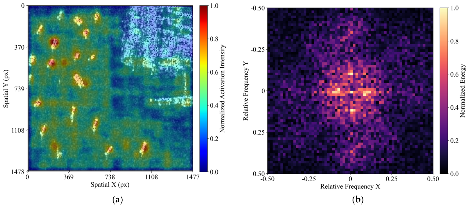
Visualization analysis shown in Figure 1 further indicates that although single–dimensional modeling provides partial improvement, scenarios persist in which the energy distributions of targets and backgrounds remain insufficiently distinguishable, increasing the risk of false positives and missed detections. Moreover, spectral energy tends to concentrate toward low–frequency regions, while high–frequency information is not adequately preserved or expressed.

Accordingly, frequency–domain modulation should be formulated as:

$${\tilde{F}}_{c,u,v}=g(c,u,v)F_{c,u,v}$$

where the modulation function depends jointly on channel–wise scattering patterns and spatial frequency subspaces, thereby establishing a three–dimensional spectral consistency constraint. Under this formulation, frequency–domain modulation is transformed from a “local denoising operation” into a “structural feature regularization mechanism,” in which noise is simultaneously suppressed along both spatial and channel dimensions, while target–related frequency bands are collaboratively preserved within target–dominant channels.

From the perspective of feature representation structure, the following core viewpoint is advanced: frequency–domain modulation in SAR detection should not be regarded as a single–dimensional local enhancement operation, but rather reformulated as a cross–dimensional and cross–level joint modeling problem. A spatial–channel joint spectral modeling framework, termed FSMD–Net, is therefore constructed, elevating frequency–domain modulation from localized feature refinement to a structural feature constraint mechanism embedded throughout multi–scale propagation. Furthermore, spectral modulation is guided by detection objectives, such that frequency components irrelevant to ship discrimination are selectively suppressed, while responses associated with weak and small targets are reinforced, rather than performing generic enhancement.

Based on this principle, a Spectral–Consistent Feature Pyramid (SCFP) module is designed within the feature pyramid architecture. During multi–scale fusion, cooperative modulation between spatial frequency–domain denoising and multi–spectral channel modeling is introduced, ensuring that features follow consistent spectral constraints during top–down propagation and preventing cumulative noise amplification across scales.

In the backbone feature extraction stage, an FFT–ResNet structure is incorporated to realize amplitude–phase collaborative spectral modeling. By establishing coupling relationships between amplitude and phase in the frequency domain, the network’s capability to represent structural boundaries and scattering patterns is enhanced.

By integrating joint spectral modeling throughout the multi–scale feature propagation process, the proposed approach differs from existing methods that primarily focus on single–dimensional or single–level frequency enhancement. Frequency–domain modulation is thereby transformed from an auxiliary denoising strategy into a structural feature regularization paradigm embedded throughout the multi–scale representation hierarchy, providing a novel representation and modulation paradigm for complex inshore SAR ship detection.

3. Methodology

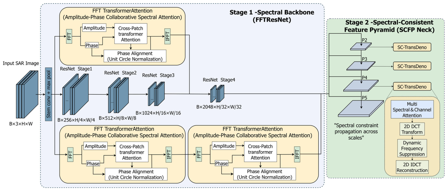
The proposed FSMD–Net consists of three components: a spectral–enhanced backbone network (Spectral Backbone), a spectral–consistent feature pyramid (SCFP Neck), and a generic detection head (Detection Head). As illustrated in Figure 2, for a given input image $I\in {ℝ}^{H_0\times W_0\times C_0}$, the forward propagation of the network can be written as:

$$D=\mathrm{Head} (\mathrm{SCFP} (\mathrm{Backbone} (I)))$$

where $D={(b_i,c_i,s_i)}_{(i=1)}^N$ denotes the detection outputs, including the bounding box b_i, category label c_i, and confidence score s_i.

The core contribution lies in the joint spectral modeling mechanism established between Backbone(⋅) and SCFP(⋅). The detection head may adopt existing one–stage or two–stage architectures without altering the proposed spectral modeling framework; therefore, it is not explicitly illustrated.

3.1. FFT–ResNet Backbone

The backbone network extracts a multi–scale feature set $\{F2 ,F3 ,F4 ,F5\}$ from the input image. Built upon a standard convolutional backbone, the computation follows the conventional “stem + multi–stage residual blocks” pipeline. To alleviate the low–frequency bias and structural detail attenuation observed during deep propagation of SAR features, frequency–domain amplitude–phase collaborative enhancement is introduced at the feature extraction stage. This design enables controllable modulation of spectral structures beyond local linear filtering in the spatial domain.

Let the output feature at a given stage be denoted as:

$$X\in {\mathrm{R}}^{\mathrm{B}\times \mathrm{C}\times H\times W}$$

where B denotes the batch size and C represents the number of channels.

Given an input feature map $X\in {\mathrm{R}}^{\mathrm{B}\times \mathrm{C}\times H\times W}$, the FFT–based spectral enhancement module first transforms it into the complex Fourier domain:

$$F=\mathrm{FFTShift}\left({\mathcal{F}}_2(X)\right)$$

where ${\mathcal{F}}_2(\cdot )$ denotes the two–dimensional Fourier transform and $\mathrm{FFTShift}(\cdot )$ shifts the zero–frequency component to the center of the spectrum. The centered spectrum is then decomposed into amplitude and phase components:

$$A=\left|F\right|,\hspace{1em}\hspace{1em}\mathrm{\Phi }=\angle F$$

Instead of directly learning the raw phase variable, the phase is embedded by its sine and cosine components to improve numerical stability:

$$P_{\sin }=\sin (\mathrm{\Phi }),\hspace{1em}\hspace{1em}{P}_{\cos }=\cos (\mathrm{\Phi })$$

The amplitude branch and the phase branch are then processed by patch–wise cross–branch attention. Specifically, the spectral descriptors are partitioned into non–overlapping spatial patches, unfolded into token sequences, and updated through cross–attention so that amplitude selectively incorporates structural cues from phase and vice versa. This process can be written as:

$$\widehat{A},{\widehat{P}}_{\sin }={\mathcal{T}}_1(A,P_{\sin })$$

$$\tilde{A},{\widehat{P}}_{\cos }={\mathcal{T}}_2(\widehat{A},P_{\cos })$$

where ${\mathcal{T}}_1(\cdot )$ and ${\mathcal{T}}_2(\cdot )$ denote two successive patch–wise cross–attention operators. For a pair of patch token sequences $Z_A$ and $Z_P$, the cross–attention operation is formulated as:

$$Q_A,K_A,V_A={\psi }_A(Z_A),\hspace{1em}\hspace{1em}{Q}_P,K_P,V_P={\psi }_P(Z_P)$$

$${\mathrm{Attn}}_{A\leftarrow P}=\mathrm{Softmax}\left({\displaystyle \frac{Q_A{K}_P^{\top }}{\sqrt{d}}}\right),\hspace{1em}\hspace{1em}{\mathrm{Attn}}_{P\leftarrow A}=\mathrm{Softmax}\left({\displaystyle \frac{Q_P{K}_A^{\top }}{\sqrt{d}}}\right)$$

$$Z_{A^{\prime }}={\mathrm{Attn}}_{A\leftarrow P}{V}_P,\hspace{1em}\hspace{1em}{Z}_{P^{\prime }}={\mathrm{Attn}}_{P\leftarrow A}{V}_A$$

To ensure phase consistency after attention modulation, the updated sine and cosine components are further normalized onto the unit circle:

$$P_{{\sin }^{\prime }}={\displaystyle \frac{{\widehat{P}}_{\sin }}{\sqrt{{\widehat{P}}_{{\sin }^2}+{\widehat{P}}_{{\cos }^2}}}},\hspace{1em}\hspace{1em}{P}_{{\cos }^{\prime }}={\displaystyle \frac{{\widehat{P}}_{\cos }}{\sqrt{{\widehat{P}}_{{\sin }^2}+{\widehat{P}}_{{\cos }^2}}}}$$

The enhanced complex spectrum is then reconstructed as:

$$\tilde{F}=\tilde{A}\cdot P_{{\cos }^{\prime }}+j\tilde{A}\cdot P_{{\sin }^{\prime }}$$

and mapped back to the spatial domain through inverse Fourier transform:

$$Y=\Re \left({\mathcal{F}}_2^{-1}\left(\mathrm{IFFTShift}(\tilde{F})\right)\right)$$

Finally, a ReLU activation is applied to obtain the enhanced output feature:

$$X_{\mathrm{out}}=\mathrm{ReLU}(Y)$$

In the actual implementation, this FFT–based spectral enhancement is inserted after the stem and after each ResNet stage output, rather than being densely applied to every intermediate convolutional block. Therefore, the backbone spectral modulation is stage–wise and sparse, which helps control the additional computational overhead.

3.2. Spectral–Consistent Feature Pyramid with Joint Channel–Spatial Denoising (SCFP)

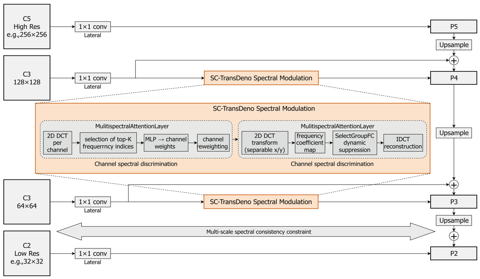
In SAR ship detection, the separability of small targets strongly depends on high–resolution feature layers. Although the top–down fusion in FPN injects high–level semantic information, it also propagates noise and background textures to high–resolution branches, resulting in cumulative noise amplification across scales. Therefore, SCFP is introduced into the feature pyramid to ensure that the fused features consistently satisfy unified spectral constraints during propagation, as illustrated in Figure 3.

SCFP takes the backbone outputs {F_i} as input and generates pyramid outputs {P_i}:

$$\{P_2,P_3,P_4,P_5\}=\mathrm{SCFP}\{F_2,F_3,F_4,F_5\}$$

The key distinction lies in the insertion of a joint spectral modulation unit, termed SC–TransDeno, into the intermediate features obtained from top–down fusion. This module enforces a cascaded constraint consisting of channel–wise spectral discriminative recalibration and spatial frequency–domain learnable denoising. The design does not rely on additional supervision; instead, it is implemented as a feature transformation module trained end–to–end.

Let the feature at the i–th scale of the backbone be denoted as $F_i\in {ℝ}^{B\times C_i\times H_i\times W_i}$. A $1\times 1$ convolution is first applied for lateral projection to obtain features with a unified channel dimension C:

$$L_i={\varphi }_i(F_i)\hspace{1em}\hspace{1em}\hspace{1em}\hspace{1em}{\varphi }_i:{ℝ}^{C_i\times H_i\times W_i}\to {ℝ}^{C\times H_i\times W_i}$$

Subsequently, top–down fusion is performed. The highest–level fused feature is initialized as:

$${\tilde{L}}_{\max }=L_{\max }$$

For the remaining layers, the fusion is recursively computed from high to low levels as:

$${\tilde{L}}_i=L_i+\mathrm{Up}({\tilde{L}}_{i+1})$$

where Up(⋅) denotes a 2× upsampling operation (e.g., nearest–neighbor or bilinear interpolation) to ensure spatial resolution alignment. This fusion process progressively propagates high–level semantic information to high–resolution layers and constitutes a critical pathway for improving small–object detection. However, it simultaneously injects high–level noise and background interference into finer–resolution features, thereby necessitating additional constraints.

It should be noted that spectral modulation is not required at all scales. The primary benefits of spectral denoising and channel discriminative enhancement are concentrated in high–resolution fusion layers, where rich texture details and speckle noise energy coexist, small–target structural details occupy a larger proportion, and cross–scale propagation is most susceptible to noise amplification.

Accordingly, at a set of selected key layers (denoted as S), the fused features are further processed by SC–TransDeno:

$${\tilde{L}}_i=\left\{\begin{array}{ll}\mathrm{SC} - \mathrm{TransDeno} ({\tilde{L}}_i),\hfill & i\in S,\hfill \\ {\tilde{L}}_i,\hfill & i\notin S.\hfill \end{array}\right.$$

The objective of this operation is not to simply enhance a specific frequency band, but to establish a consistent “noise suppression–structure preservation” criterion across both channel and spatial dimensions, thereby avoiding over–suppression or over–enhancement caused by single–dimensional modulation.

Finally, to suppress aliasing effects introduced during fusion and to unify the output representation, a $3\times 3$ convolutional smoothing operation is applied at each scale:

$$P_i={\psi }_i({\tilde{L}}_i)\hspace{1em}\hspace{1em}\hspace{1em}\hspace{1em} {\psi }_i:{ℝ}^{C_i\times H_i\times W_i}\to {ℝ}^{C\times H_i\times W_i}$$

The results are fed into the detection head for classification and regression. In this manner, SCFP embeds joint spectral modeling into the multi–scale propagation pathway without modifying the detection head or the overall training framework.

3.3. SC–TransDeno: Multi–Spectral Channel Attention and Learnable Denoising in the Spatial DCT Domain

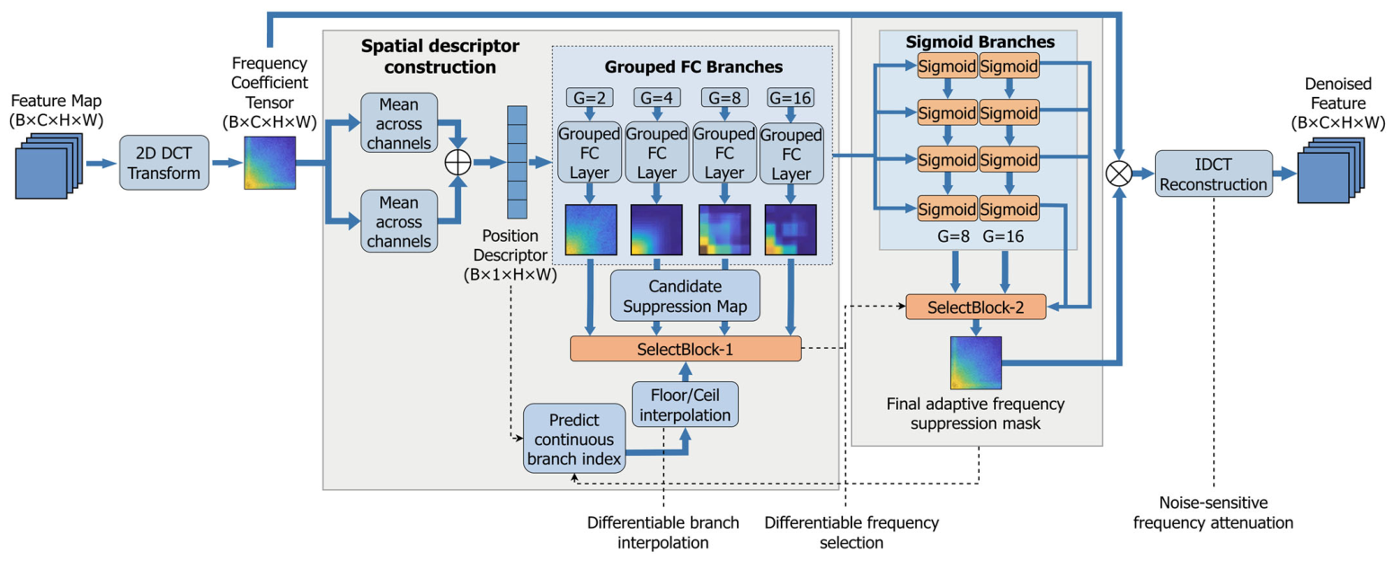
SC–TransDeno serves as the core modulation unit within SCFP, as illustrated in Figure 4. Its design follows a clear sequential principle: channel modulation precedes spatial modulation. Intuitively, the channel dimension characterizes scattering patterns and semantic subspaces. Performing discriminative spectral weighting along the channel dimension first prevents spatial frequency–domain denoising from excessively shrinking target–sensitive channels. Subsequently, learnable denoising is conducted in the spatial frequency domain to further suppress speckle noise and high–frequency clutter, thereby achieving cooperative enhancement.

Given an input $X\in {ℝ}^{B\times C\times H\times W}$, the overall mapping of SC–TransDeno is expressed as:

$$Y={\mathrm{IDCT}}_{2D}(G({\mathrm{DCT}}_{2D}(\mathrm{MSCA}(x))))$$

where $\mathrm{MSCA}(\cdot )$ denotes multi–spectral channel attention, $\mathrm{DCT}2D(\cdot )$ and $\mathrm{IDCT}2D(\cdot )$ represent the two–dimensional orthogonal transform and its inverse, respectively, and denotes the frequency–domain suppressor implemented in a dynamically selected soft–threshold or soft–suppression form.

Conventional channel attention mechanisms (e.g., SE) obtain channel descriptors via global average pooling (GAP). For two–dimensional signals, GAP is equivalent to retaining only the zero–frequency component of the discrete cosine transform (DCT), which can be formally expressed as:

$$\mathrm{GAP}(X_c)={\displaystyle \frac{1}{HW}}{\displaystyle \sum _{x=0}^{H-1}{\displaystyle \sum _{y=0}^{W-1}{X}_c}}(x,y)$$

However, the discriminative cues of SAR ship targets are not confined to extremely low–frequency average energy, but also reside in a set of representative mid– and low–frequency or directionally sensitive components. To address this, MSCA selects a set of frequency indices in the two–dimensional DCT domain:

$$\mathrm{\Omega }={\{(u_k,v_k)\}}_{k=1}^K$$

and extracts the coefficients at these selected frequency locations for each channel as the channel descriptor.

In the present implementation, the frequency index set Ω is predefined rather than learned during training. Specifically, following the frequency–selection strategy of FcaNet, we adopt a fixed set of K = 16 representative DCT frequency components selected from a canonical 7 × 7 frequency grid:

$$\mathrm{\Omega }={\{(u_k,v_k)\}}_{k=1}^K,\hspace{1em}\hspace{1em}K=16$$

The selected base coordinates are fixed during training and shared across all datasets.

$$\begin{gathered} \left(0,0\right), \left(0,1\right), \left(6,0\right), \left(0,5\right), \left(0,2\right), \left(1,0\right), \left(1,2\right), \left(4,0\right), \\ \left(5,0\right), \left(1,6\right), \left(3,0\right), \left(0,4\right), \left(0,6\right), \left(0,3\right), \left(3,5\right), \left(2,2\right). \end{gathered}$$

For feature maps of different spatial resolutions, the coordinates are proportionally rescaled rather than relearned, so that the same relative frequency positions are preserved across layers:

$$(u_k^{(l)},v_k^{(l)})=\left(⌊{\displaystyle \frac{H_l}{7}}{u}_k⌋,⌊{\displaystyle \frac{W_l}{7}}{v}_k⌋\right),\hspace{1em}\hspace{1em}k=1,\dots ,K$$

where $H_l$ and $W_l$ denote the spatial size of the l–th feature level. Therefore, the current MSCA design corresponds to a fixed–frequency and cross–layer consistent channel–spectrum modeling strategy.

The two–dimensional DCT orthogonal basis functions are defined (with normalization coefficient denoted as $\alpha (\cdot )$) as:

$${\varphi }_{u,v}(x,y)=\alpha (u)\alpha (v)\cos \left({\displaystyle \frac{\pi (2x+1)u}{2H}}\right)\cos \left({\displaystyle \frac{\pi (2y+1)v}{2W}}\right)$$

The coefficient of channel $\left(C\right)$ at the frequency location $\left(u_k, v_k\right)$ is given by:

$$d_{c,k}={\displaystyle \sum _{x=0}^{H-1}{\displaystyle \sum _{y=0}^{W-1}{X}_c}}(x,y){\varphi }_{u_k,v_k}(x,y)$$

The coefficients at the selected frequency locations are concatenated to form the channel descriptor vector:

$$z_c=[d_{c,1},\dots ,d_{c,K}]\in {ℝ}^K$$

Channel weights are then generated through a two–layer learnable mapping (following the SE paradigm, while extending the input from a scalar to a multi–frequency vector):

$$w_c=\sigma (w_2^T\delta (W_1{z}_c)),c=1,\dots ,C$$

where $\delta (\cdot )$ denotes a nonlinear activation function (e.g., ReLU or GELU), and $\sigma (\cdot )$ denotes the sigmoid function. Channel recalibration is then performed as follows:

$${X^{\prime }}_c=w_c\cdot X_c\hspace{1em}\hspace{1em}\hspace{1em}\hspace{1em}\hspace{1em} X^{\prime }=X\odot w$$

Here, $w=[w_1,\dots ,w_C]$ is broadcast along the channel dimension to the spatial domain. The function of MSCA can be interpreted as redistributing feature energy into scattering–mode subspaces that are more relevant to target characteristics before spatial frequency–domain denoising is applied, thereby reducing the likelihood of subsequent spatial suppression incorrectly attenuating weak target–sensitive channels.

After obtaining the channel–weighted feature $X^{\mathrm{\prime }}$, SC–TransDeno maps it into the spatial frequency subspace. In the actual implementation, the spatial frequency projection is realized by a separable two–dimensional discrete cosine transform (2D–DCT), which is sequentially performed along the width and height dimensions using precomputed orthogonal cosine bases. The two–dimensional DCT can be written as:

$$X_f=\mathcal{D}(X^{\prime })$$

where $\mathcal{D}(\cdot )$ denotes the two–dimensional orthogonal transform defined above, and denotes the tensor of frequency–domain coefficients. In practice, the separability of the DCT can be exploited for efficient computation. For the channel–weighted feature $X\prime \in {\mathrm{R}}^{\mathrm{B}\times \mathrm{C}\times H\times W}$, the width–direction transform is first applied:

$$X_{b,c,i,v}^{(x)}={\displaystyle \sum _{j=0}^{W-1}{X^{\prime }}_{b,c,i,j}}{\beta }_W(v,j)$$

Then, the height–direction transform is applied to obtain the final DCT–domain coefficient tensor:

$$X_{f b,c,u,v}={\displaystyle \sum _{i=0}^{H-1}{X}_{b,c,i,v}^{(x)}}{\beta }_H(u,i)$$

where the orthogonal cosine bases are defined as:

$${\beta }_W(v,j)={\alpha }_W(v)\cos \left({\displaystyle \frac{\pi (2j+1)v}{2W}}\right)$$

$${\beta }_H(u,i)={\alpha }_H(u)\cos \left({\displaystyle \frac{\pi (2i+1)u}{2H}}\right)$$

$${\alpha }_W(v)=\left\{\begin{array}{ll}{\displaystyle \frac{1}{\sqrt{W}}},\hfill & v=0\hfill \\ [4pt]\sqrt{{\displaystyle \frac{2}{W}}},\hfill & v>0\hfill \end{array}\right.,\hspace{1em}\hspace{1em}{\alpha }_H(u)=\left\{\begin{array}{ll}{\displaystyle \frac{1}{\sqrt{H}}},\hfill & u=0\hfill \\ [4pt]\sqrt{{\displaystyle \frac{2}{H}}},\hfill & u>0\hfill \end{array}\right.$$

Thereby, the two–dimensional projection is decomposed into two successive one–dimensional projections, which preserves the orthogonality of the transform while enabling efficient implementation. Here, $X_f$ denotes the tensor of frequency–domain coefficients. The low–frequency region typically carries background structural information and the main–body energy of targets, whereas the mid– and high–frequency regions contain edge details and broadband speckle noise components.

Denoising of $X_f$ is not performed using a fixed threshold; instead, a content–adaptive soft suppression strategy is adopted. The key idea is to generate a suppression weight map $\mathrm{A}$ each frequency location based on the frequency–domain statistics of the current sample. This suppression map is shared across all channels, enabling consistent structural shrinkage in the frequency domain:

$${\tilde{X}}_f=A\odot X_f$$

To ensure sufficient expressive capacity of A, it is generated through a mechanism combining multiple grouped candidate mappings with differentiable selection. This design can be conceptually described as a two–stage process.

First, $X_f$ is aggregated along the channel dimension to obtain location–wise statistics, reflecting the overall energy and peak intensity at each spatial (or frequency–domain) coordinate:

$$y_{b,n,1}={\displaystyle \frac{1}{C}}{\displaystyle \sum _{c=1}^C{X}_{f b,c}}(n)+{\max }_{1\le c\le C}{X}_{f b,c}(n),\hspace{1em}\hspace{1em}n=1,\dots ,HW$$

where $n$ denotes the flattened frequency–position index. This statistic simultaneously captures the average energy and maximum response, which facilitates the distinction between “structurally concentrated frequency bands” and “noise–like random fluctuations.”

A set of candidate mapping functions is then constructed over the frequency–position sequence. In the actual implementation, these mappings are instantiated as lightweight grouped one–dimensional convolution branches rather than an unspecified generic family of one– or two–dimensional operators.

Based on the location–wise statistic y, the first–stage candidate mappings are defined as:

$$f_m(y)=\delta \left(\mathrm{Conv}1{\mathrm{D}}_{g_m}(y)\right),\hspace{1em}\hspace{1em}{g}_m\in \{2,4,8,16\},\hspace{1em}m=1,\dots ,4$$

where $\delta (\cdot )$ denotes the ReLU activation. Different candidate mappings correspond to different assumptions regarding subspace granularity. Smaller group numbers impose stronger parameter sharing and tend to enforce globally consistent suppression, whereas larger group numbers allow finer–grained local frequency adaptation.

To avoid the non–differentiability introduced by discrete branch selection, a differentiable soft–selection operator is introduced to interpolate among the candidate branches. The fused intermediate representation is written as:

$$t={\mathcal{S}}_1(y,{\{f_m(y)\}}_{m=1}^4)$$

where ${\mathcal{S}}_1(\cdot )$ denotes the first soft–selection operator. This process can be interpreted as a continuous selection among candidate subspaces, allowing the effective granularity of frequency modeling to be adaptively adjusted according to the input content.

Based on the fused feature $t$, the second–stage candidate mappings are further constructed as

$$g_m(t)=\sigma \left(\mathrm{Conv}1{\mathrm{D}}_{g_m}(t)\right),\hspace{1em}\hspace{1em}{g}_m\in \{2,4,8,16\},\hspace{1em}m=1,\dots ,4$$

where $\sigma (\cdot )$ denotes the sigmoid activation. A second differentiable selector then generates the final suppression map:

$$A={\mathcal{S}}_2(t,{\{g_m(t)\}}_{m=1}^4)$$

where ${\mathcal{S}}_2(\cdot )$ denotes the second soft–selection operator. The suppression map is shared across all channels and applied to the DCT–domain coefficients by element–wise modulation:

$${\tilde{X}}_f=A\odot X_f$$

This frequency–domain suppression process can be interpreted as a content–adaptive soft–threshold shrinkage mechanism. When certain frequency locations exhibit noise–like spikes or non–structural high–frequency dispersion, $A$ tends to attenuate their responses. Conversely, when spectral energy presents continuous, directional, or target–related structural concentration, $A$ tends to preserve and enhance those components.

Finally, an inverse DCT is applied to the suppressed frequency coefficients to reconstruct the spatial–domain feature:

$$Y={\mathcal{D}}^{-1}({\tilde{X}}_f)$$

Since the DCT is an orthogonal transform, ${\mathcal{D}}^{-1}(\cdot )$ can be regarded as the inverse mapping of $\mathcal{D}(\cdot )$, ensuring that frequency–domain modulation corresponds to an interpretable and energy–controllable reconstruction process in the spatial domain. The resulting output $Y$ is returned to the feature propagation pathway of the FPN and is subsequently fed into the detection head together with features from other scales.

4. Experiments and Discussion

4.1. Experimental Datasets

The experiments in this section are designed to systematically evaluate the effectiveness and generalization capability of the proposed joint spatial–channel spectral modeling approach on representative SAR ship detection benchmarks.

In particular, it is investigated whether the introduction of channel–domain spectral modeling can improve detection accuracy—especially for ship targets—while maintaining the stability of the overall network architecture. Evaluations are conducted on three representative complex–scene SAR datasets: SARDet–100K, HRSID, and AIR–SARShip–2.0.

SARDet–100K is an open–source benchmark constructed for large–scale SAR object detection, aiming to provide a unified evaluation standard under complex and high–density scenarios [10]. The dataset contains 43,819 SAR images with more than 100,000 annotated object instances, covering diverse scene types and imaging conditions. Target categories include ships as well as other typical SAR objects. The images are acquired from multiple spaceborne SAR sensors, with spatial resolutions ranging from sub–meter to several meters. Scenes include inshore areas, ports, islands, and open seas, featuring complex backgrounds. The dataset exhibits large–scale variation, a high proportion of small objects, and significant strong–scattering structures and clutter interference, making it an important benchmark for evaluating multi–scale robustness and generalization performance.

HRSID (High–Resolution SAR Image Dataset) is a widely used high–resolution SAR ship detection dataset [9]. It consists of 136 large–scene SAR images with spatial resolutions ranging from 1 to 5 m. These large scenes are cropped into 5604 sub–images containing 16,951 annotated ship targets. The dataset covers both inshore and offshore scenarios. In inshore regions, complex backgrounds and dense strong–scattering structures coexist with small–scale ships and shoreline interference, leading to increased detection difficulty. Horizontal bounding boxes are adopted for annotation. Due to imbalanced scale distribution and a high proportion of small targets, HRSID is frequently used to assess fine–grained recognition capability and robustness against background interference.

AIR–SARShip–2.0 is an extended version of the AIR–SARShip dataset, specifically constructed for ship detection in complex inshore environments [32]. It contains 300 high–resolution SAR images covering ports, coastal areas, islands, and near–shore scenes, with approximately 2000 annotated ship targets. The spatial resolution is mainly at meter level. Targets are generally small and exhibit varying contrast levels. Unlike open–sea datasets, ships in AIR–SARShip–2.0 are often interwoven with shoreline buildings, strong–scattering objects, and sea clutter. The complex background structure and weak target–background separability make this dataset particularly suitable for evaluating detection stability and practical adaptability under strong interference and small–object conditions.

4.2. Experimental Environment and Implementation Details

Experiments were conducted on a Windows platform equipped with an NVIDIA RTX 4090D Laptop GPU, with CUDA runtime version 12.8. The deep learning framework was implemented using Python 3.8.20 and PyTorch 2.0.1. The CUDA backend utilized pytorch–cuda 11.8 and relied on official acceleration libraries including cuBLAS, cuFFT, and cuDNN to ensure computational efficiency and numerical stability.

Numerical computation and tensor operations were primarily supported by NumPy 1.24.3 and the Intel MKL acceleration library. Image processing operations were implemented using standard libraries such as Pillow. All experiments were conducted within the same Python virtual environment to guarantee identical runtime conditions for different models during training and evaluation.

For methodological rigor, all compared methods adopted unified data preprocessing pipelines, loss function formulations, and training strategies.

4.3. Experimental Results

mAP refers to COCO–style mAP@[0.5:0.95]; mAP(07) denotes VOC2007 mAP@0.5 used for consistency with prior baselines on certain splits. “IN” indicates ImageNet–pretrained backbones; all CNN–based baselines follow the same pretraining setting for fair comparison.

Table 1. Comparison with state–of–the–art (SOTA) methods on the SARDet–100K.

Model	Pre.	mAP	mAP@0.5	mAP@0.75	mAP_s	mAP_m	mAP_l
One–stage
YOLOF	IN	0.474	0.788	0.503	0.391	0.626	0.561
FCOS	IN	0.525	0.858	0.549	0.471	0.661	0.578
GFL	IN	0.551	0.851	0.589	0.494	0.673	0.605
RepPoints	IN	0.517	0.864	0.540	0.467	0.633	0.538
ATSS	IN	0.550	0.876	0.583	0.499	0.679	0.590
CenterNet	IN	0.539	0.862	0.573	0.489	0.662	0.577
PAA	IN	0.522	0.857	0.548	0.460	0.639	0.576
TOOD	IN	0.547	0.869	0.584	0.502	0.667	0.586
DDOD	IN	0.540	0.866	0.572	0.493	0.647	0.580
VFNet	IN	0.530	0.843	0.563	0.474	0.654	0.580
AutoAssign	IN	0.540	0.896	0.560	0.501	0.634	0.547
Two–stage
Faster R–CNN	IN	0.392	0.700	0.399	0.326	0.472	0.420
Cascade R–CNN	IN	0.536	0.873	0.568	0.491	0.629	0.487
Dynamic R–CNN	IN	0.498	0.810	0.539	0.431	0.597	0.548
Grid R–CNN	IN	0.501	0.806	0.535	0.424	0.620	0.527
Libra R–CNN	IN	0.521	0.835	0.558	0.459	0.635	0.554
ConvNeXt	IN	0.532	0.855	0.573	0.457	0.646	0.586
ConvNeXtV2	IN	0.539	0.860	0.589	0.476	0.647	0.596
LSKNet	IN	0.524	0.851	0.570	0.452	0.636	0.592
End2end
DenoDet	IN	0.559	0.858	0.602	0.506	0.685	0.610
FSMD–Net (ours)	IN	0.565	0.864	0.609	0.507	0.691	0.611

Bold values indicate the best result in each column.

presents the quantitative comparison between FSMD–Net and representative state–of–the–art (SOTA) methods on the SARDet–100K dataset. From an overall performance perspective, DenoDet, which is based on spatial frequency–domain analysis, achieves significant improvements over conventional methods, demonstrating the effectiveness of frequency–domain feature denoising in large–scale SAR ship detection tasks. Building upon this foundation, FSMD–Net further improves the mAP from 0.559 to 0.565, while also achieving gains in both mAP@0.5 and mAP@0.75. These results indicate that joint spatial–channel spectral modeling can continuously enhance detection performance without compromising the stability of the original detection framework.

Analysis across different object scales reveals that the primary performance gains are concentrated on small and medium–sized targets. FSMD–Net outperforms DenoDet in both mAP_s and mAP_m, whereas improvements for large targets (mAP_l) are relatively limited. This observation suggests that multi–spectral channel modeling is more effective in preserving high–frequency discriminative information associated with small–scale ships during spectral compression and feature recalibration, thereby alleviating the suppression of weak target responses caused by spatial frequency–domain denoising.

Table 2. Comparison with SOTA methods on the HRSID.

Model	mAP	mAP@0.5	mAP@0.75	mAP_s	mAP_m	mAP_l
One–stage
YOLOF	0.233	0.490	0.188	0.248	0.208	0.025
SRDet	0.705	0.906	0.802	0.714	0.720	0.360
DSDet	0.605	0.907	0.746	0.668	0.640	0.076
Two–stage
HRSDNet	0.694	0.893	0.798	0.703	0.711	0.289
CenterNet2	0.694	0.895	0.794	0.700	0.714	0.375
End2end
DenoDet	0.561	0.800	0.624	0.562	0.632	0.304
FSMD–Net(ours)	0.575	0.813	0.638	0.576	0.640	0.314

Bold values indicate the best result in each column.

summarizes the experimental results of different methods on the HRSID dataset. It can be observed that in high–resolution scenes characterized by complex inshore environments and strong–scattering backgrounds, the detection performance of YOLOF is significantly limited. In contrast, DenoDet achieves notable improvements in overall accuracy by incorporating spatial frequency–domain denoising. Furthermore, FSMD–Net attains the best performance across the mAP, mAP@0.5, and mAP@0.75 metrics, with the overall mAP increasing from 0.561 to 0.575.

It is particularly noteworthy that, compared with DenoDet, FSMD–Net exhibits a more pronounced improvement in small–object detection performance on HRSID, achieving an mAP_s of 0.576. This result suggests that under complex inshore backgrounds with strong–scattering interference, spectral response discrepancies across channels become more significant. Reliance solely on spatial frequency–domain denoising is insufficient to fully exploit discriminative information. By introducing multi–spectral modeling along the channel dimension, target–relevant channel responses can be more effectively enhanced, thereby improving the stability of small and weak ship detection.

Table 3. Comparison with SOTA methods on the AIR–SARShip–2.0.

Model	Pre.	mAP	mAP@0.5	mAP@0.75
One–stage
RetinaNet	IN	0.206	0.577	0.065
FCOS	IN	0.222	0.590	0.102
GFL	IN	0.255	0.581	0.146
YOLOv3–t	IN	0.350	0.755	0.389
Two–stage
Faster–RCNN	IN	0.359	0.723	0.290
Cascade–RCNN	IN	0.325	0.732	0.325
Grid–RCNN	IN	0.302	0.685	0.205
Libra–RCNN	IN	0.240	0.590	0.124
End2end
ATSS	IN	0.274	0.645	0.179
CenterNet	IN	0.133	0.416	0.035
DINO	IN	0.261	0.538	0.160
RTD–Det–R50	IN	0.329	0.662	0.271
DenoDet	IN	0.348	0.733	0.288
FSMD–Net (ours)	IN	0.379	0.756	0.343

Bold values indicate the best result in each column.

presents the quantitative comparison between FSMD–Net and representative methods on the AIR–SARShip–2.0 dataset. AIR–SARShip–2.0 is characterized by complex inshore backgrounds, strong–scattering interference, and uneven target scale distribution, thereby imposing stricter requirements on model robustness and discriminative capability.

In comparison, DenoDet, which incorporates spatial frequency–domain denoising, achieves substantial performance improvements on AIR–SARShip–2.0, reaching an mAP of 0.348 and an mAP@0.5 of 0.733. These results verify the effectiveness of frequency–domain feature denoising in suppressing strong clutter interference and enhancing target responses. Building upon this foundation, FSMD–Net further achieves the best overall detection accuracy, with mAP increasing to 0.379 and mAP@0.75 significantly improving from 0.288 to 0.343. These improvements indicate that joint spatial–channel spectral modeling provides stronger advantages in precise localization and confidence discrimination.

4.4. Ablation Study

The ablation study is conducted to analyze the individual and combined effects of the spatial frequency–domain denoising module (SFD) and different channel attention modeling strategies (CA–GAP and CA–MS) on SAR ship detection performance. By progressively introducing these components, their respective contributions to detection accuracy are systematically evaluated. The corresponding experimental configurations are summarized in

Table 4. Ablation Study on the Necessity of Spatial Frequency–Domain Denoising and Multi–Spectral Channel Attention.

SFD	CA–GAP	CA–MS	SARDet–100K	HRSID	AIR–SARShip–2.0
			mAP(07)	mAP(07)	mAP(07)
×	×	×	0.525	0.271	0.220
√	×	×	0.533	0.553	0.321
√	√	×	0.559	0.561	0.348
√	×	√	0.565	0.575	0.379

√ and × denote whether the corresponding module is enabled or disabled, respectively.

, where the complete model corresponds to the configuration in which both spatial frequency–domain denoising and multi–spectral channel attention (SFD + CA–MS) are simultaneously enabled.

To verify the necessity of spatial frequency–domain denoising (SFD), a baseline detection framework without any frequency–domain modeling or channel attention mechanism is first adopted as a reference. Based on this baseline, only the SFD module is enabled for comparison. This configuration is designed to examine whether introducing feature modulation from the pure spatial domain into the frequency domain can yield stable performance gains without altering the channel modeling strategy.

Subsequently, upon incorporating SFD, two different channel modeling strategies are further compared: channel attention based on global average pooling (CA–GAP) and channel attention based on multi–spectral compression (CA–MS). CA–GAP represents the conventional channel attention paradigm, whose channel compression process is equivalent in the frequency domain to retaining only the lowest–frequency component. In contrast, CA–MS models channel spectral information more comprehensively by introducing multiple representative frequency components. This comparison aims to investigate whether different channel spectral modeling strategies exert distinct impacts on detection performance when spatial frequency–domain denoising is already present.

Furthermore, by comparing the configurations “SFD + CA–GAP” and “SFD + CA–MS,” the potential advantages of multi–spectral channel attention in terms of spectral modulation consistency and small–target feature preservation can be analyzed. This design directly corresponds to the central hypothesis that spatial–only frequency–domain denoising remains incomplete, and that incorporating channel–domain multi–spectral modeling more effectively distinguishes target–relevant channels from background–interference channels, particularly improving detection stability for small–scale ship targets in complex scenes.

Finally, the complete configuration enabling both spatial frequency–domain denoising and multi–spectral channel attention is adopted as the final model to validate the overall effectiveness of the joint spatial–channel spectral modeling strategy. This configuration corresponds to the last row in Table 4 and represents the full implementation of FSMD–Net. Through comparison with the aforementioned simplified variants, the contributions of each module to overall performance improvement can be systematically evaluated, and their synergistic effects under different dataset conditions can be analyzed.

The experimental results indicate that introducing SFD alone yields significant performance gains across all three datasets. On SARDet–100K, the mAP increases from 0.525 to 0.533. On HRSID, performance improves substantially from 0.271 to 0.553. On AIR–SARShip–2.0, the mAP rises from 0.220 to 0.321. Notably, the improvements are more pronounced on complex inshore datasets such as HRSID and AIR–SARShip–2.0, demonstrating that spatial frequency–domain modulation effectively suppresses speckle noise and enhances target responses under strong–scattering backgrounds.

After introducing CA–GAP, the mAP further increases to 0.559, 0.561, and 0.348 on SARDet–100K, HRSID, and AIR–SARShip–2.0, respectively, compared with the configuration using SFD alone. This observation suggests that channel recalibration following frequency–domain denoising helps alleviate channel–response imbalance, thereby improving overall detection performance.

When CA–MS replaces CA–GAP, performance continues to improve to 0.565 on SARDet–100K, 0.575 on HRSID, and 0.379 on AIR–SARShip–2.0. In particular, the notable improvement on AIR–SARShip–2.0 indicates that relying solely on the lowest–frequency component for channel compression is insufficient to capture channel spectral discrepancies in complex inshore environments, whereas multi–spectral modeling preserves frequency information more relevant to target discrimination.

To further clarify the internal design of the multi–spectral channel attention (CA–MS) module, an additional ablation study is conducted on the number of selected DCT frequency locations, denoted by K. In the present implementation, the frequency index set is constructed according to the fixed frequency–selection strategy introduced in FcaNet. Specifically, let Ω rank denote the predefined ordered frequency list on the canonical 7 × 7 DCT grid. Then, the frequency index set used in MSCA is defined by selecting the first K coordinates from this fixed ranking. These frequency coordinates are not learned during training, but are fixed a priori and shared across datasets. For feature maps of different spatial resolutions, the same relative frequency positions are preserved through proportional coordinate scaling rather than frequency re–selection. Therefore, this experiment aims to examine how the descriptor size K affects detection performance under a deterministic and reproducible frequency–selection rule.

Table 5. Ablation Study of the Number of Selected DCT Frequency Locations K in MSCA on HRSID.

K	mAP	mAP@50	mAP@75	mAP_s	mAP_m	mAP_l
1	0.566	0.798	0.631	0.569	0.626	0.248
2	0.561	0.793	0.624	0.564	0.614	0.196
4	0.565	0.802	0.622	0.569	0.608	0.257
8	0.572	0.808	0.638	0.575	0.625	0.280
16	0.569	0.803	0.631	0.571	0.635	0.261
32	0.570	0.801	0.638	0.574	0.616	0.208

Bold values indicate the best result in each column.

reports the ablation results on HRSID with $K\in \{1,2,4,8,16,32\}$, while keeping all other training and evaluation settings unchanged. A clear trend can be observed. When K is very small, the channel–frequency descriptor is overly sparse and cannot adequately characterize the diverse spectral responses of ship targets and surrounding clutter. As K increases from 1 or 2 to 8, the overall detection performance improves accordingly. The best overall result is achieved at K = 8, where the model attains 0.572 mAP, 0.808 mAP@0.5, and 0.638 mAP@0.75. When K is further increased to 16 or 32, the performance remains highly competitive but no longer improves consistently. In particular, the default setting K = 16 achieves 0.569 mAP, which is only 0.003 lower than the best result obtained at K = 8. This observation indicates that once K reaches a moderate range, the proposed method becomes relatively insensitive to the exact value of K.

From a modeling perspective, this behavior is consistent with the functional role of MSCA. An excessively small K under–represents the spectral diversity of channel responses, whereas an overly large K introduces more redundant frequency components and may weaken the compactness of channel attention. A moderate K therefore provides a better balance between spectral descriptiveness and robustness to clutter interference.

This ablation study further supports the rationality of the adopted fixed top–K frequency–selection strategy and demonstrates that the proposed CA–MS design remains stable for moderate values of K.

Overall, the ablation results demonstrate that spatial frequency–domain denoising provides a strong foundation for suppressing clutter interference, while the incorporation of channel spectral modeling further enhances detection performance by improving channel discriminability. The comparison between CA–GAP and CA–MS confirms that multi–spectral channel modeling is more effective than conventional lowest–frequency channel compression, especially in complex inshore scenarios. Moreover, the additional analysis on the frequency descriptor size K shows that the proposed CA–MS design remains stable within a moderate range of frequency selections, further supporting the rationality and robustness of the adopted fixed top–K strategy. Therefore, the complete model achieves the best overall performance by jointly exploiting complementary spatial and channel spectral information.

4.5. Computational Complexity and Efficiency Analysis

To evaluate the computational overhead introduced by FSMD–Net, we compare it with the baseline DenoDet in terms of FLOPs, parameter count, activation size, inference latency, and GPU memory usage under identical experimental settings.

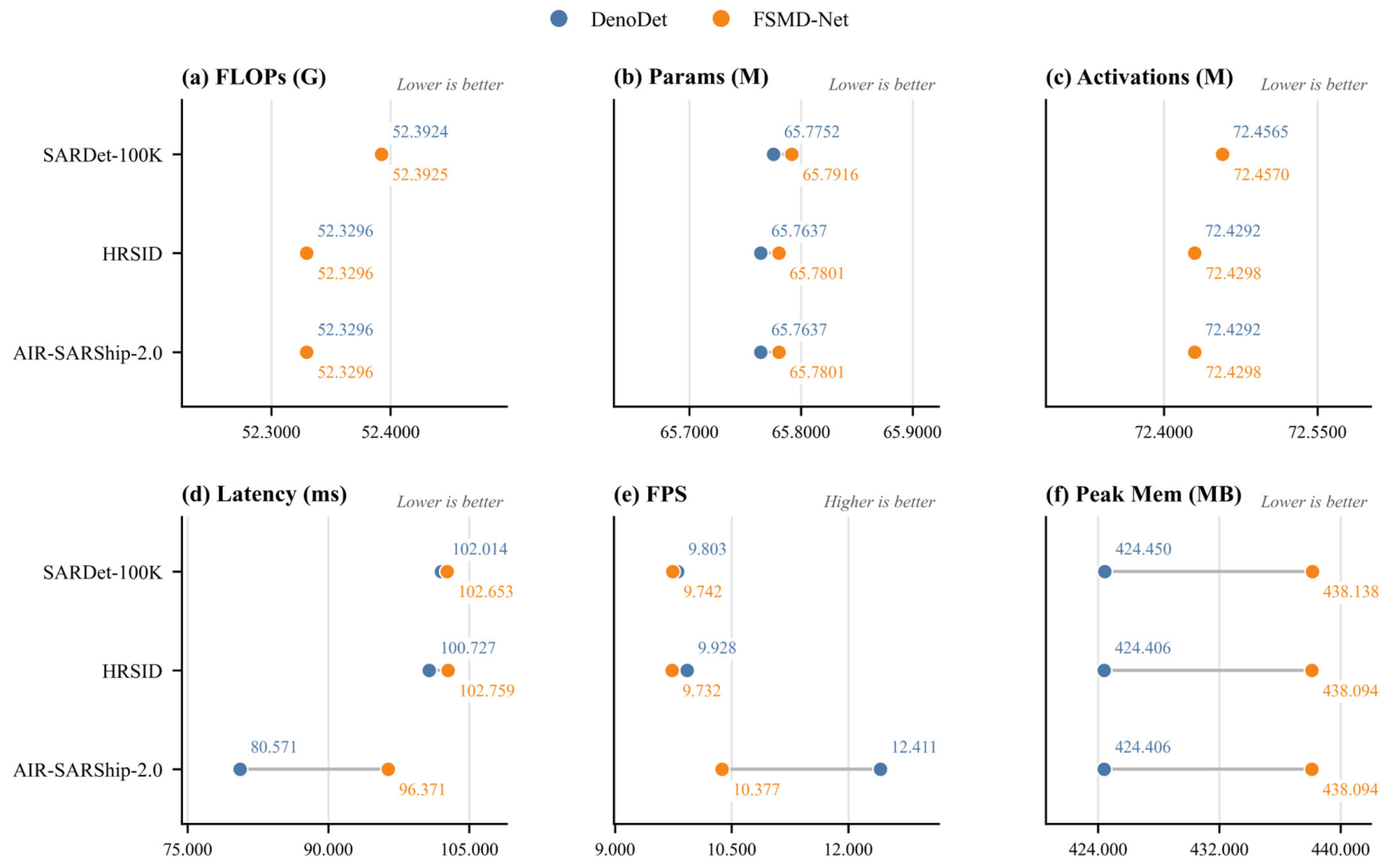
The results, as illustrated in

Table 6. Comparison of theoretical computational complexity and practical inference efficiency between DenoDet and FSMD–Net.

Datasets	Model	FLOPs(G)	Params (M)	Activations (M)	Latency (ms)	FPS	Peak Mem (MB)
SARDet–100K	DenoDet	52.392444	65.775247	72.456496	102.014492	9.802529	424.450195
	FSMDnet (Ours)	52.392460	65.791631	72.457040	102.653118	9.741545	438.137695
HRSID	DenoDet	52.329591	65.763722	72.429216	100.727285	9.927797	424.406250
	FSMDnet (Ours)	52.329607	65.780106	72.429760	102.759006	9.731507	438.093750
AIR–SARship–2.0	DenoDet	52.329591	65.763722	72.429216	80.570813	12.411442	424.406250
	FSMDnet (Ours)	52.329607	65.780106	72.429760	96.371194	10.376545	438.093750

and Figure 5, indicate that the proposed spectral modeling introduces negligible theoretical complexity. Across all datasets, the increase in FLOPs is approximately 0.000016 G, corresponding to less than 0.001%. The parameter count increases by only 0.016 M, demonstrating that the performance gain is not achieved through model scaling.

In terms of practical efficiency, the runtime overhead remains limited. On SARDet–100K and HRSID, the latency increase is within 2%, while GPU memory consumption increases by approximately 3%. Although a larger latency variation is observed on AIR–SARShip–2.0, this discrepancy is attributed to hardware–dependent runtime factors rather than architectural complexity.

Overall, FSMD–Net achieves improved detection performance with nearly unchanged theoretical complexity and only marginal practical overhead, validating the efficiency of the proposed design.

4.6. Phase Contribution and Internal Visualization Analysis

To further elucidate the internal working mechanism of the proposed joint spectral modeling framework, this section provides a comprehensive analysis from two complementary perspectives:

The explicit contribution of phase information to structural preservation, and the internal feature modulation process of MSCA and SC–TransDeno through multi–level visualization. All visualizations are generated under identical normalization settings for fair comparison.

4.6.1. Phase Contribution to Structural Representation

In the proposed FFT–ResNet backbone, spectral features are decomposed into amplitude and phase components, which are jointly modulated through cross–attention. While amplitude primarily reflects energy distribution, phase encodes spatial structure, including boundary location and geometric configuration.

To quantitatively and qualitatively analyze the role of phase, three reconstruction strategies are compared:

(1)

Full–spectrum reconstruction;

(2)

Amplitude–only reconstruction;

(3)

Phase–only reconstruction.

$$Reconstruction=F^{-1}(A,\varphi )$$

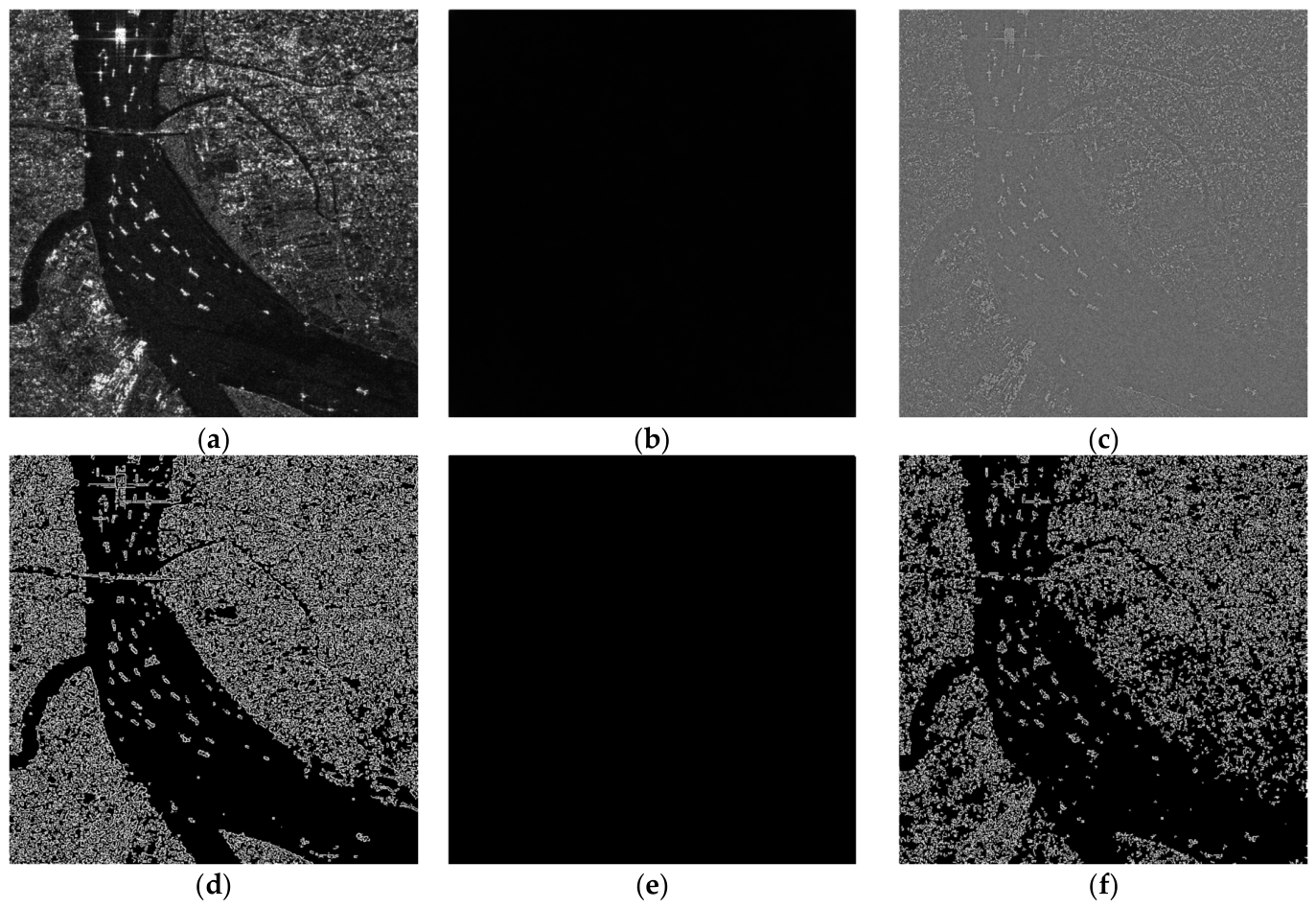
The experimental results demonstrate a clear distinction between amplitude and phase contributions as illustrated in Figure 6. Amplitude–only reconstruction preserves coarse intensity distribution but fails to retain object contours and boundary sharpness. In contrast, phase–only reconstruction effectively preserves structural information, including ship outlines, edge continuity, and spatial arrangement.

Quantitatively, phase–only reconstruction significantly improves structural consistency. The edge F1 score, defined as the harmonic mean of edge precision and edge recall, is used to quantify the consistency between the reconstructed edge map and the reference boundary structure, thereby reflecting the ability of the reconstruction to preserve target contours and boundary geometry. For example, on representative samples from HRSID and AIR–SARShip–2.0, the edge F1 score increases from near–zero values in amplitude–only reconstruction to over 0.5 in phase–only reconstruction, while gradient correlation improves from approximately zero to above 0.8. These results indicate that phase carries dominant structural cues critical for object localization.

This observation is consistent with classical signal–processing theory, where phase is known to determine geometric structure, while amplitude controls intensity distribution. In the context of SAR ship detection, preserving phase information is therefore essential for maintaining boundary integrity under complex scattering environments.

4.6.2. Visualization of Channel–Spatial Spectral Modulation

To further clarify the internal behavior of the proposed joint spectral modeling framework, we provide detailed visualizations of the feature transformation process within the neck. Specifically, we analyze:

(1)

Channel–frequency selection in MSCA;

(2)

Spatial frequency–domain suppression in SC–TransDeno;

(3)

Multi–level feature propagation across the feature pyramid.

To ensure a fair comparison, all visualizations are conducted on the same SARDet–100K sample, and both the baseline and the proposed method are analyzed under identical settings.

(1)

Channel–Frequency Selection in MSCA

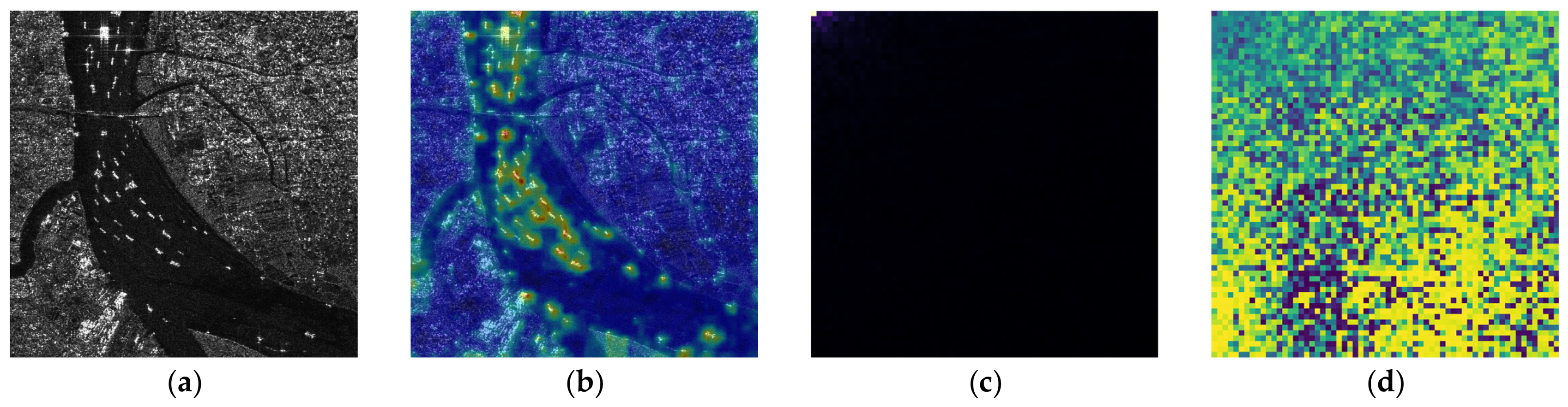
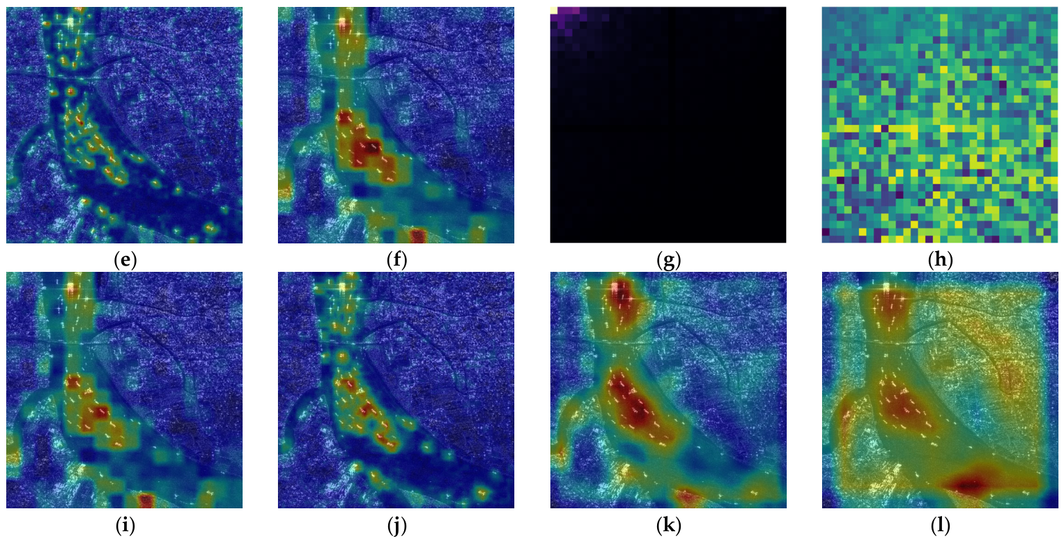
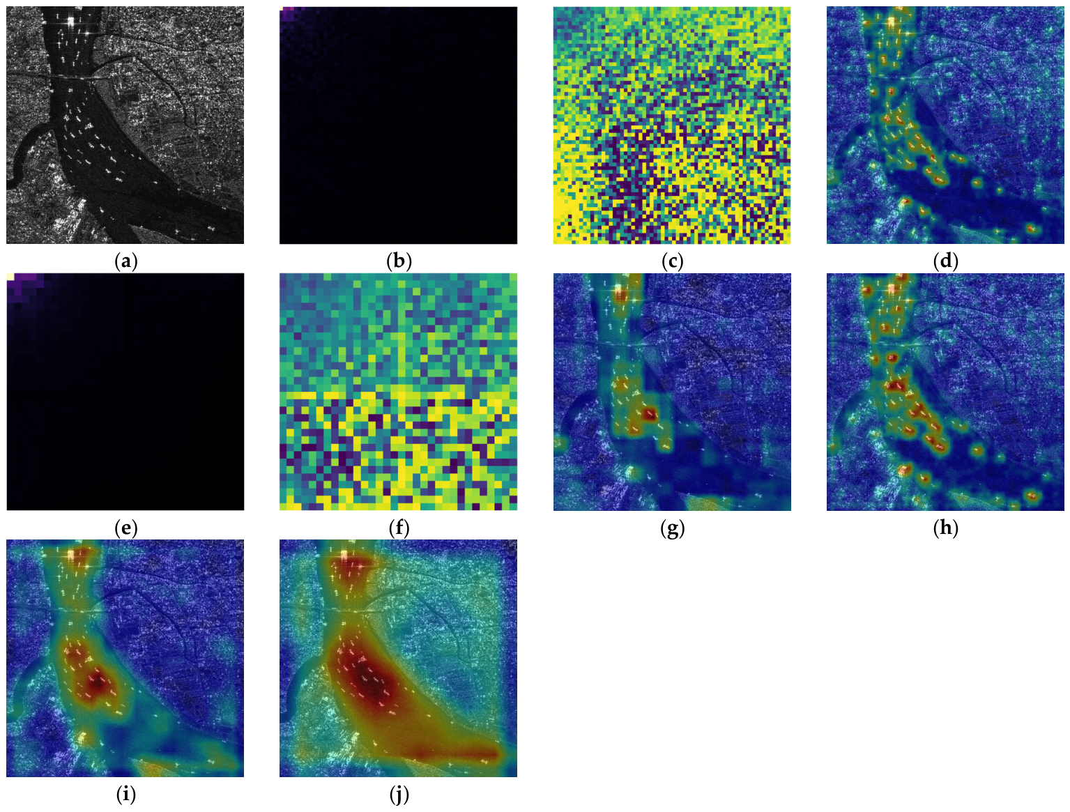
To visualize the effect of multi–spectral channel attention, we analyze the channel weights together with the corresponding DCT coefficient responses after MSCA as illustrated in Figure 7 and Figure 8.

Compared with the baseline model, which does not explicitly model channel–frequency interactions, MSCA introduces a clear dynamic selection mechanism across channels. The learned channel weights are not uniformly distributed but exhibit a wide dynamic range, indicating that different channels are selectively emphasized based on their spectral characteristics.

For instance, on the SARDet–100K sample, the two MSCA modules in FSMD–Net produce mean channel weights of 0.4800 and 0.5069, respectively, with dynamic ranges of approximately 0.9720 and 0.9745. Such large dynamic ranges demonstrate that MSCA performs strong discriminative reweighting rather than simple global scaling.

As a result, the corresponding DCT coefficient maps after MSCA become more structured and concentrated, providing a more informative spectral representation before spatial frequency–domain suppression is applied. This confirms that MSCA effectively enhances target–relevant channels while suppressing background–dominant responses.

(2)

Frequency–Domain Suppression in SC–TransDeno

We further visualize the suppression maps generated by SC–TransDeno to analyze its behavior in the spatial frequency domain.

The results show that the suppression maps are highly non–uniform and exhibit strong spatial–frequency selectivity. Instead of applying uniform attenuation across all frequency locations, the module adaptively preserves or suppresses frequency components based on their structural relevance.

On the same SARDet–100K sample, the two suppression maps generated by SC–TransDeno have mean values of 0.5514 and 0.8417, respectively, with dynamic ranges of approximately 0.9887 and 0.9948. These values indicate that the suppression process is highly content–adaptive and capable of producing near–binary–like selection behavior in the frequency domain.

This observation suggests that SC–TransDeno does not merely perform generic denoising, but instead learns a discriminative frequency filtering strategy that preserves structured spectral patterns while attenuating noise–like components.

(3)

Multi–Level Feature Pyramid Analysis

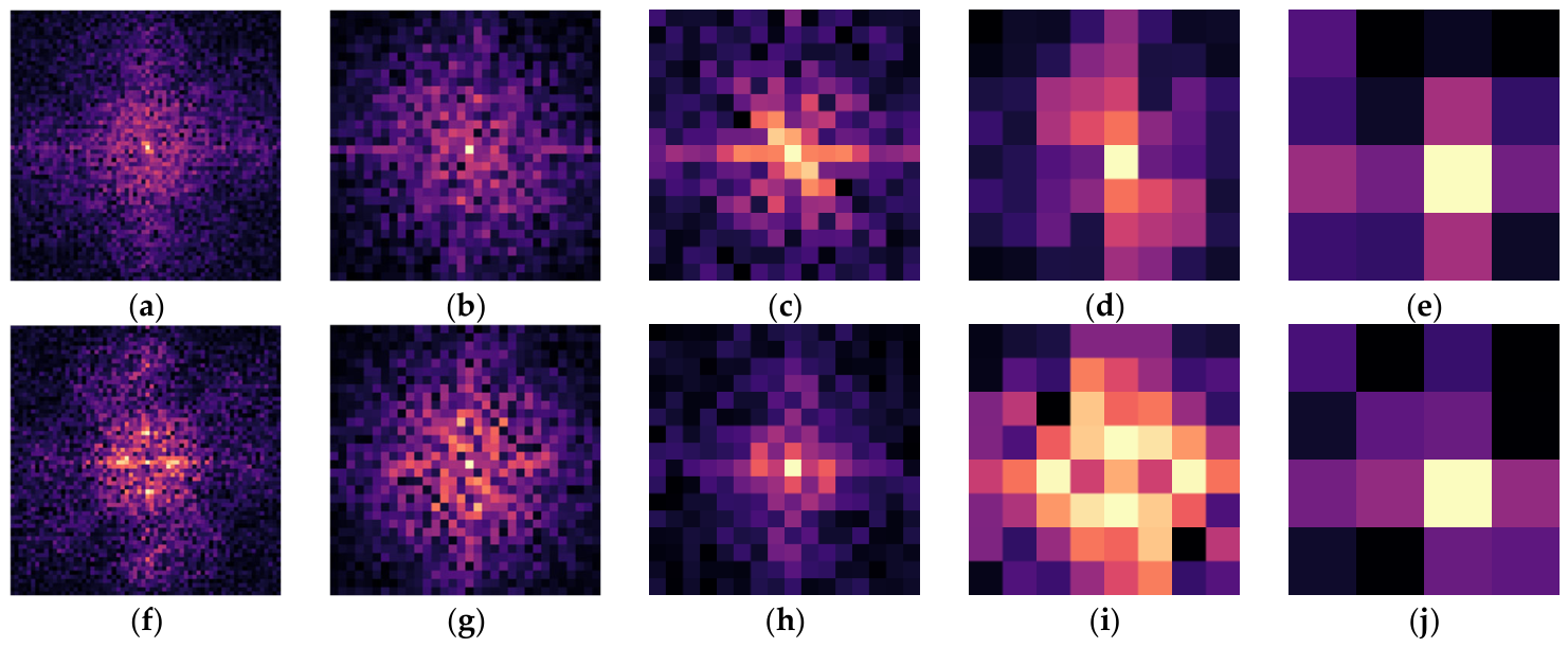
To analyze the effect of spectral modulation across different scales, we visualize the feature maps and corresponding frequency spectra at multiple pyramid levels (L0–L4) for both the baseline and FSMD–Net.

From the visualization results shown in Figure 9, several consistent patterns can be observed:

In the baseline model, feature activations are relatively diffuse and exhibit strong background interference, especially at higher–resolution levels. The corresponding frequency spectra show dispersed energy distributions with limited structural organization.

In contrast, FSMD–Net produces more target–focused activation patterns across all pyramid levels. The spatial responses become more concentrated around ship regions, while background clutter is significantly suppressed.

In the frequency domain, spectral energy distributions after modulation are more structured and exhibit clearer concentration patterns, indicating improved separation between target–related and noise–related frequency components.

These observations demonstrate that the proposed joint spectral modeling framework enforces consistent feature refinement across scales and effectively mitigates the accumulation of noise during top–down feature propagation.

(4)

Summary

Overall, the visualization results provide clear evidence that: MSCA performs discriminative channel–frequency selection before spatial modulation; SC–TransDeno implements adaptive and spatially selective frequency suppression; The combination of these modules leads to more structured spectral representations and improved target–focused responses across the feature pyramid.

4.7. Broader Discussion, Scope, and Failure Cases

The above analyses further validate the effectiveness of the proposed spectral modulation mechanism and provide an intuitive understanding of its internal operation. From a broader perspective, FSMD–Net can be positioned within the general family of frequency–domain modeling methods for SAR image analysis. Classical approaches based on predefined multi–resolution transforms, such as wavelet– or contourlet–based representations, usually rely on handcrafted basis functions to perform fixed decomposition and enhance structural characteristics such as edges, directional patterns, or multi–scale textures [33,34,35,36]. By contrast, the proposed method adopts a task–driven spectral modeling paradigm embedded into deep feature hierarchies, in which spatial frequency, channel frequency, and amplitude–phase components are jointly modulated in an end–to–end manner. Therefore, FSMD–Net should not be regarded as a replacement for classical transform–domain methods, but rather as a complementary and learnable spectral refinement mechanism operating at the feature level.

It is also necessary to clarify the scope of the current framework. In practical SAR systems, image degradation may arise not only from speckle noise and complex background clutter, but also from various forms of interference and jamming, such as deceptive jamming or multichannel interference [37,38]. These problems are typically addressed at the signal–processing level through array processing, multichannel filtering, or waveform–domain modeling, whereas the present work focuses on feature–level representation learning under single–channel imaging conditions. Although the proposed spectral modulation mechanism can adaptively suppress irregular and non–structural spectral components and may thus provide a certain degree of implicit robustness when interference appears as incoherent spectral disturbance in the feature space, explicit interference–aware modeling is beyond the scope of this study and remains an important direction for future work.

In addition, although the current implementation is built upon a ResNet backbone for fair comparison with prior work, the proposed framework is not inherently restricted to a specific architecture. The SCFP module operates on multi–scale feature maps and is largely backbone–agnostic, making it potentially compatible with modern hierarchical architectures such as ConvNeXt and Swin Transformer. For sequence–based models, including Mamba–like or tokenized transformer variants, additional adaptation is required to align frequency–domain operations with sequence representations. Nevertheless, the core principle of joint spatial–channel spectral modeling remains applicable across different backbone designs, indicating that FSMD–Net can be understood as a general and extensible spectral modulation framework.

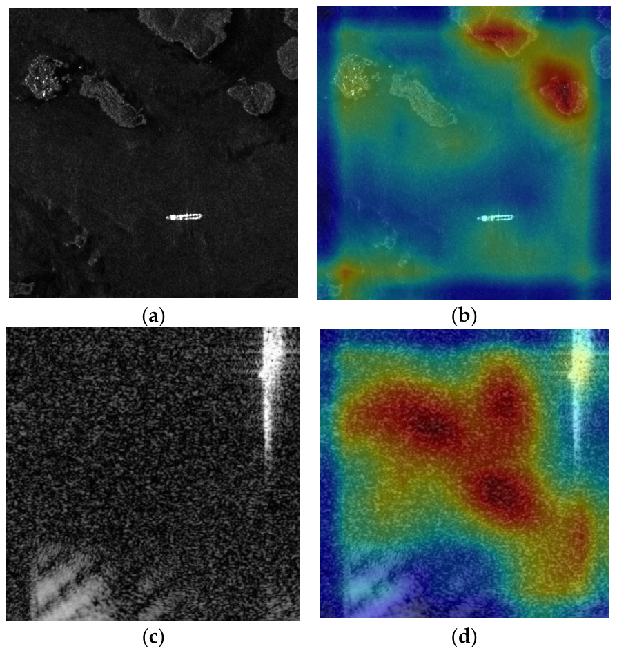
Despite these advantages, several failure cases are still observed in highly challenging scenes, as shown in Figure 10. When ships are extremely close to strong–scattering structures such as harbors, shorelines, or dense man–made facilities, the target response may remain partially entangled with background–dominant spectral components, leading to missed detections or inaccurate localization. In addition, for very weak or extremely small targets, useful structural cues may be insufficiently preserved after repeated cross–scale propagation, especially when the target–background contrast is severely degraded. These observations suggest that, although the proposed joint spectral modulation improves robustness in complex inshore environments, the separability between weak ship signatures and strongly structured background clutter is not completely resolved. More explicit interference–aware priors, stronger boundary–sensitive constraints, or cross–domain spectral adaptation may further improve performance in such cases.

5. Conclusions

This study addresses long–standing challenges in ship detection under complex SAR scenarios, with particular emphasis on speckle noise interference and insufficient detection performance for small–scale and blurred targets. In view of the limitations of existing methods in terms of frequency–domain modeling dimensionality, a joint spatial–channel spectral modeling framework, termed FSMD–Net, is proposed. Building upon feature–level frequency–domain denoising, a multi–spectral channel modeling mechanism is incorporated to enhance the discriminability and stability of feature representations.

Specifically, adaptive modulation of different frequency subspaces is performed in the frequency domain through a spatial frequency–domain denoising module, effectively suppressing interference components associated with speckle noise. Meanwhile, spectral discrepancies across the channel dimension are modeled via a multi–spectral channel attention mechanism, alleviating the information loss caused by treating all channels uniformly in conventional frequency–domain denoising. In this manner, a more balanced trade–off is achieved between noise suppression and the preservation of small–target features.

Experimental results on multiple representative SAR ship detection benchmarks demonstrate that FSMD–Net achieves consistent improvements in both overall detection accuracy and small–object performance, without introducing significant computational overhead. These findings validate the effectiveness and robustness of joint spatial–channel spectral modeling in complex inshore and strong–scattering scenarios, and provide a novel modeling perspective for future research on SAR ship detection in challenging environments.

References

1. Alexandre, C.; Devillers, R.; Mouillot, D.; Seguin, R.; Catry, T. Ship Detection With SAR C-Band Satellite Images: A Systematic Review. IEEE J. Sel. Top. Appl. Earth Obs. Remote Sens. 2024, 17, 14353–14367. [Google Scholar] [CrossRef] [Scilit]
2. Yasir, M.; Wan, J.; Xu, M.; Sheng, H.; Zeng, Z.; Liu, S.; Colak, A.T.I.; Hossain, M.S. Ship Detection Based on Deep Learning Using SAR Imagery: A Systematic Literature Review. Soft Comput. 2023, 27, 63–84. [Google Scholar] [CrossRef] [Scilit]
3. Wang, C.; Liao, M.; Li, X. Ship Detection in SAR Image Based on the Alpha-Stable Distribution. Sensors 2008, 8, 4948–4960. [Google Scholar] [CrossRef] [Scilit]
4. Zhao, Z.; Ji, K.; Xing, X.; Zou, H. Adaptive CFAR Detection of Ship Targets in High Resolution SAR Imagery. In MIPPR 2013: Multispectral Image Acquisition, Processing, and Analysis; SPIE: Bellingham, WA, USA, 2013; p. 89170L. [Google Scholar] [CrossRef] [Scilit]
5. Sun, S.; Wang, J. Ship Detection in SAR Images Based on Steady CFAR Detector and Knowledge-Oriented GBDT Classifier. Electronics 2024, 13, 2692. [Google Scholar] [CrossRef] [Scilit]
6. Meng, S.; Ren, K.; Lu, D.; Gu, G.; Chen, Q.; Lu, G. A Novel Ship CFAR Detection Algorithm Based on Adaptive Parameter Enhancement and Wake-Aided Detection in SAR Images. Infrared Phys. Technol. 2018, 89, 263–270. [Google Scholar] [CrossRef] [Scilit]
7. Mazzeo, A.; Renga, A.; Graziano, M.D. A Systematic Review of Ship Wake Detection Methods in Satellite Imagery. Remote Sens. 2024, 16, 3775. [Google Scholar] [CrossRef] [Scilit]
8. Zhang, T.; Zhang, X.; Li, J.; Xu, X.; Wang, B.; Zhan, X.; Xu, Y.; Ke, X.; Zeng, T.; Su, H.; et al. SAR Ship Detection Dataset (SSDD): Official Release and Comprehensive Data Analysis. Remote Sens. 2021, 13, 3690. [Google Scholar] [CrossRef] [Scilit]
9. Wei, S.; Zeng, X.; Qu, Q.; Wang, M.; Su, H.; Shi, J. HRSID: A High-Resolution SAR Images Dataset for Ship Detection and Instance Segmentation. IEEE Access 2020, 8, 120234–120254. [Google Scholar] [CrossRef] [Scilit]
10. Cheng, M.-M.; Hou, Q.; Li, W.; Li, X.; Li, Y.; Liu, L.; Yang, J. SARDet-100K: Towards Open-Source Benchmark and ToolKit for Large-Scale SAR Object Detection. In Proceedings of the Advances in Neural Information Processing Systems 37; Neural Information Processing Systems Foundation, Inc. (NeurIPS): Vancouver, BC, Canada, 2024; pp. 128430–128461. [Google Scholar]
11. Liu, W.; Anguelov, D.; Erhan, D.; Szegedy, C.; Reed, S.; Fu, C.-Y.; Berg, A.C. SSD: Single Shot MultiBox Detector. In Computer Vision–ECCV 2016; Leibe, B., Matas, J., Sebe, N., Welling, M., Eds.; Lecture Notes in Computer Science; Springer International Publishing: Cham, Switzerland, 2016; Volume 9905, pp. 21–37. ISBN 978-3-319-46447-3. [Google Scholar]
12. Redmon, J.; Farhadi, A. YOLOv3: An Incremental Improvement. arXiv 2018, arXiv:1804.02767. [Google Scholar] [CrossRef] [Scilit]
13. Lin, T.-Y.; Dollar, P.; Girshick, R.; He, K.; Hariharan, B.; Belongie, S. Feature Pyramid Networks for Object Detection. In Proceedings of the 2017 IEEE Conference on Computer Vision and Pattern Recognition (CVPR); IEEE: Honolulu, HI, USA, 2017; pp. 936–944. [Google Scholar]
14. Lin, T.-Y.; Goyal, P.; Girshick, R.; He, K.; Dollar, P. Focal Loss for Dense Object Detection. In Proceedings of the 2017 IEEE International Conference on Computer Vision (ICCV); IEEE: Venice, Italy, 2017; pp. 2999–3007. [Google Scholar]
15. Tian, Z.; Shen, C.; Chen, H.; He, T. FCOS: Fully Convolutional One-Stage Object Detection. In Proceedings of the 2019 IEEE/CVF International Conference on Computer Vision (ICCV); IEEE: Seoul, Republic of Korea, 2019; pp. 9626–9635. [Google Scholar]
16. Zhang, S.; Chi, C.; Yao, Y.; Lei, Z.; Li, S.Z. Bridging the Gap Between Anchor-Based and Anchor-Free Detection via Adaptive Training Sample Selection. In Proceedings of the 2020 IEEE/CVF Conference on Computer Vision and Pattern Recognition (CVPR); IEEE: Seattle, WA, USA, 2020; pp. 9756–9765. [Google Scholar]
17. Chang, Y.-L.; Anagaw, A.; Chang, L.; Wang, Y.C.; Hsiao, C.-Y.; Lee, W.-H. Ship Detection Based on YOLOv2 for SAR Imagery. Remote Sens. 2019, 11, 786. [Google Scholar] [CrossRef] [Scilit]
18. Sun, Z.; Leng, X.; Lei, Y.; Xiong, B.; Ji, K.; Kuang, G. BiFA-YOLO: A Novel YOLO-Based Method for Arbitrary-Oriented Ship Detection in High-Resolution SAR Images. Remote Sens. 2021, 13, 4209. [Google Scholar] [CrossRef] [Scilit]
19. Yu, C.; Shin, Y. SAR Ship Detection Based on Improved YOLOv5 and BiFPN. ICT Express 2024, 10, 28–33. [Google Scholar] [CrossRef] [Scilit]
20. Girshick, R. Fast R-CNN. In Proceedings of the 2015 IEEE International Conference on Computer Vision (ICCV); IEEE: Santiago, Chile, 2015; pp. 1440–1448. [Google Scholar]
21. Ren, S.; He, K.; Girshick, R.; Sun, J. Faster R-CNN: Towards Real-Time Object Detection with Region Proposal Networks. IEEE Trans. Pattern Anal. Mach. Intell. 2017, 39, 1137–1149. [Google Scholar] [CrossRef] [Scilit] [PubMed]
22. Liu, L.; Pan, Z.; Lei, B. Learning a Rotation Invariant Detector with Rotatable Bounding Box. arXiv 2017, arXiv:1711.09405. [Google Scholar] [CrossRef] [Scilit]
23. Han, J.; Ding, J.; Li, J.; Xia, G.-S. Align Deep Features for Oriented Object Detection. arXiv 2020, arXiv:2008.09397. [Google Scholar] [CrossRef] [Scilit]
24. Yu, X.; Lin, M.; Lu, J.; Ou, L. Oriented Object Detection in Aerial Images Based on Area Ratio of Parallelogram. arXiv 2021, arXiv:2109.10187. [Google Scholar] [CrossRef] [Scilit]
25. Carion, N.; Massa, F.; Synnaeve, G.; Usunier, N.; Kirillov, A.; Zagoruyko, S. End-to-End Object Detection with Transformers. arXiv 2020, arXiv:2005.12872. [Google Scholar]
26. Zhu, X.; Su, W.; Lu, L.; Li, B.; Wang, X.; Dai, J. Deformable DETR: Deformable Transformers for End-to-End Object Detection. arXiv 2021, arXiv:2010.04159. [Google Scholar]
27. Dai, Y.; Zou, M.; Li, Y.; Li, X.; Ni, K.; Yang, J. DenoDet: Attention as Deformable Multisubspace Feature Denoising for Target Detection in SAR Images. IEEE Trans. Aerosp. Electron. Syst. 2025, 61, 4729–4743. [Google Scholar] [CrossRef] [Scilit]
28. Zhou, Y.; Liu, H.; Ma, F.; Pan, Z.; Zhang, F. A Sidelobe-Aware Small Ship Detection Network for Synthetic Aperture Radar Imagery. IEEE Trans. Geosci. Remote Sens. 2023, 61, 5205516. [Google Scholar] [CrossRef] [Scilit]
29. Qin, Z.; Zhang, P.; Wu, F.; Li, X. FcaNet: Frequency Channel Attention Networks. In Proceedings of the 2021 IEEE/CVF International Conference on Computer Vision (ICCV); IEEE: Montreal, QC, Canada, 2021; pp. 763–772. [Google Scholar]
30. Oppenheim, A.V.; Lim, J.S. The Importance of Phase in Signals. Proc. IEEE 1981, 69, 529–541. [Google Scholar] [CrossRef] [Scilit]
31. Ni, X.S.; Huo, X. Statistical Interpretation of the Importance of Phase Information in Signal and Image Reconstruction. Stat. Probab. Lett. 2007, 77, 447–454. [Google Scholar] [CrossRef] [Scilit]
32. Sun, X.; Wang, Z.; Sun, Y. AIR-SARShip-1.0: High-Resolution SAR Ship Detection Dataset. J. Radars 2019, 8, 852–862. [Google Scholar] [CrossRef]
33. Singh, P.; Shankar, A.; Diwakar, M. Review on Nontraditional Perspectives of Synthetic Aperture Radar Image Despeckling. J. Electron. Imaging 2022, 32, 021609. [Google Scholar] [CrossRef] [Scilit]
34. Liu, G.; Kang, H.; Wang, Q.; Tian, Y.; Wan, B. Contourlet-CNN for SAR Image Despeckling. Remote Sens. 2021, 13, 764. [Google Scholar] [CrossRef] [Scilit]
35. Choi, H.; Jeong, J. Speckle Noise Reduction Technique for SAR Images Using Statistical Characteristics of Speckle Noise and Discrete Wavelet Transform. Remote Sens. 2019, 11, 1184. [Google Scholar] [CrossRef] [Scilit]
36. Huang, Y.; Xin, Z.; Liao, G.; Huang, P.; Hou, G.; Zou, R. Unsupervised SAR Image Change Detection Based on Curvelet Fusion and Local Patch Similarity Information Clustering. Remote Sens. 2025, 17, 840. [Google Scholar] [CrossRef] [Scilit]
37. Xiao, Z.; He, F.; Sun, Z.; Zhang, Z. Mitigation of Suppressive Interference in AMPC SAR Based on Digital Beamforming. Remote Sens. 2024, 16, 2812. [Google Scholar] [CrossRef] [Scilit]
38. Chang, S.; Tang, S.; Deng, Y.; Zhang, H.; Liu, D.; Wang, W. An Advanced Scheme for Deceptive Jammer Localization and Suppression in Elevation Multichannel SAR for Underdetermined Scenarios. IEEE Trans. Aerosp. Electron. Syst. 2026, 62, 3952–3970. [Google Scholar] [CrossRef] [Scilit]
Figure 1. Output heatmap of spatial attention combined with channel–wise average pooling (a) and the corresponding spatial frequency–domain energy distribution (b).
Remotesensing 18 01254 g001
Figure 2. Overview of the FSMD–Net architecture.
Remotesensing 18 01254 g002
Figure 3. Architecture of the SCFP module. The circled plus symbol denotes element–wise feature fusion by addition.
Remotesensing 18 01254 g003
Figure 4. Internal structure of the Multi–Spectral Attention Layer. The circled plus symbol denotes element–wise addition for descriptor fusion, while the circled multiplication symbol denotes element–wise multiplication for adaptive frequency modulation.
Remotesensing 18 01254 g004
Figure 5. Comparison of theoretical computational complexity and practical inference efficiency between DenoDet and FSMD–Net. Subfigures (ac) present the theoretical complexity metrics, including FLOPs, parameter count, and activation size, while subfigures (df) report the practical inference efficiency in terms of latency, frames per second (FPS), and peak GPU memory usage. Blue markers denote the baseline DenoDet, and orange markers denote the proposed FSMD–Net. For FLOPs, parameters, activations, latency, and peak memory, lower values indicate better efficiency, whereas for FPS, higher values are preferable.
Remotesensing 18 01254 g005
Figure 6. Comparison of full–spectrum, amplitude–only, and phase–only reconstruction on representative SAR samples. (a) Original image; (b) Amplitude–only reconstruction; (c) Phase–only reconstruction; (d) edges original map; (e) edges map—amplitude only; (f) edges map—phase only.
Remotesensing 18 01254 g006
Figure 7. Internal visualization of spectral denoising in the baseline model. (a) Input SAR image patch; (b) DCT coefficients without MSCA in spectral branch 1; (c) suppression map A in spectral branch 1; (d) IDCT–reconstructed feature in spectral branch 1; (e) DCT coefficients without MSCA in spectral branch 2; (f) suppression map A in spectral branch 2; (g) IDCT–reconstructed feature in spectral branch 2; (h) pyramid–level activation at L0; (i) pyramid–level activation at L1; (j) pyramid–level activation at L2.
Remotesensing 18 01254 g007
Figure 8. Internal visualization of MSCA–guided spectral modulation and multi–scale feature responses in FSMD–Net. (a) Input SAR image patch; (b) MSCA–enhanced activation in spectral branch 1; (c) DCT coefficients after MSCA in spectral branch 1; (d) Learned suppression map A in spectral branch 1; (e) IDCT–reconstructed feature in spectral branch 1; (f) MSCA–enhanced activation in spectral branch 2; (g) DCT coefficients after MSCA in spectral branch 2; (h) Learned suppression map A in spectral branch 2; (i) IDCT–reconstructed feature in spectral branch 2; (j) Pyramid–level feature activation at L0; (k) Pyramid–level feature activation at L1; (l) Pyramid–level feature activation at L2.
Remotesensing 18 01254 g008aRemotesensing 18 01254 g008b
Figure 9. Pyramid–level frequency–spectrum comparison between the baseline DenoDet and FSMD–Net on the HRSID sample. (ae) Frequency spectra of the baseline model at pyramid levels L0–L4. (fj) Frequency spectra of FSMD–Net at pyramid levels L0–L4 after spectral modulation.
Remotesensing 18 01254 g009
Figure 10. Representative failure cases of FSMD–Net in challenging SAR scenes. (a) Original input image of a representative failure case in a complex inshore HRSID scene. (b) Detection result of FSMD–Net for the scene shown in (a). (c) Original input image of a representative failure case under severe noise contamination. (d) Detection result of FSMD–Net for the scene shown in (c).
Remotesensing 18 01254 g010