Semi-Supervised Remote Sensing Image Semantic Segmentation Based on Multi-Scale Consistency and Cross-Attention

Highlights

What are the main findings?

• The proposed MSCA-TSN effectively improves semi-supervised remote sensing image segmentation by integrating uncertainty-aware multi-scale consistency learning and cross-network attention interaction.
• Extensive experiments on the LoveDA and ISPRS Potsdam datasets demonstrate that MSCA-TSN achieves superior segmentation accuracy and boundary integrity under limited supervision, reaching up to 52.41% mIoU on LoveDA and 76.34% mIoU on Potsdam with only 10% labeled data.

What are the implications of the main findings?

• The results indicate that uncertainty-guided multi-scale feature consistency can effectively suppress noisy supervision and enhance the robustness of semi-supervised segmentation in complex remote sensing scenes.
• The proposed cross-teacher–student attention interaction provides a promising direction for improving discriminative feature learning in semi-supervised remote sensing tasks, especially when labeled data are scarce.

Abstract

Remote sensing image (RSI) semantic segmentation is challenged by high inter-class spectral similarity, significant intra-class scale variation, and limited availability of labeled data. Although semi-supervised learning has reduced the dependency on large-scale annotations, existing approaches still suffer from degraded boundary precision and incomplete geometric structures in complex remote sensing scenes. To address these issues, this paper proposes a Multi-scale Consistency and Cross-Attention Teacher–Student Network (MSCA-TSN) for semi-supervised RSI semantic segmentation. Specifically, an Adaptive Multi-scale Uncertainty Consistency module (AMUC) is introduced to model feature reliability across hierarchical levels. By leveraging Monte Carlo Dropout to estimate feature uncertainty and employing adaptive weighting for multi-scale consistency learning, AMUC effectively suppresses unreliable supervision and improves segmentation robustness under significant scale variations. Furthermore, a Cross-Teacher–Student Cross-Attention Module (CCAM) is designed to enhance cross-network feature interaction. In CCAM, student features act as queries while teacher features serve as keys and values to construct cross-attention, enabling the student network to reconstruct more discriminative feature representations and reduce confusion among visually similar land-cover categories. Extensive experiments are conducted on the LoveDA and ISPRS Potsdam benchmarks under both 5% and 10% labeling ratios. On the LoveDA dataset, MSCA-TSN achieves mIoU scores of 51.05% and 52.41% under 5% and 10% labeled data, respectively, outperforming several state-of-the-art semi-supervised methods. On the ISPRS Potsdam dataset, the proposed method further reaches 75.35% and 76.34% mIoU under the same settings. Ablation and parameter sensitivity analyses further verify the effectiveness and robustness of the proposed AMUC and CCAM modules.

1. Introduction

Semantic segmentation is a fundamental task in analyzing remote sensing images (RSIs) and is widely applied in applications such as land use planning, urban expansion monitoring, agricultural crop distribution analysis, and disaster assessment [1,2,3,4]. Advances in remote sensing technologies, including satellites and unmanned aerial vehicles, have led to higher resolutions and broader imaging swaths, resulting in RSIs with increased complexity and volume [5,6,7]. This advancement places higher demands on segmentation algorithms to accurately capture detailed target information while enhancing interpretation precision, especially in scenarios with limited annotated data. Traditional semi-supervised semantic segmentation methods for RSIs face inherent limitations in effectively handling these complex data, often failing to generalize well and maintain segmentation accuracy due to the unique characteristics of RSIs [8,9]. When dense pixel-level annotations are difficult to obtain, low-supervision paradigms such as weakly supervised and semi-supervised segmentation become increasingly attractive, as they attempt to reduce annotation cost while preserving dense prediction capability. For example, weakly supervised studies have shown that sparse supervision can still provide useful guidance for segmentation, although such settings usually rely on much weaker annotation forms and are therefore different from the semi-supervised scenario studied in this paper [10].

Convolutional neural network (CNN)-based encoder-decoder architectures, including FCN [11], SegNet [12], and UNet [13], have achieved remarkable performance in semantic segmentation and have been widely extended to RSI analysis [8,14]. These hierarchical convolution operations enable automatic learning of abstract features from pixels to semantics, improving segmentation accuracy in complex remote sensing scenes. Extending these techniques to RSIs, various improved methods have demonstrated significant improvements in feature extraction and segmentation precision. Despite these successes, challenges persist in modeling the rich contextual information embedded in RSIs, particularly high inter-class feature similarity and significant intra-class scale variation [15,16]. More recently, Transformer-based segmentation models have also demonstrated strong global context modeling ability, and semi-supervised studies such as AllSpark further explored architecture-level cross-attention designs in a Transformer framework [17]. However, in remote sensing semi-supervised segmentation with very limited annotations, CNN-based teacher–student frameworks remain a strong and stable choice due to their comparatively mature optimization behavior and strong locality-aware inductive bias. In this work, we therefore focus on improving the teacher–student learning mechanism on a CNN-based segmentation framework, while discussing Transformer-related developments more specifically in Section 2.

Multi-scale context aggregation methods have further advanced RSI semantic segmentation by employing strategies such as pyramid pooling and dilated convolutions to capture information across different spatial scales [15,16,18]. These methods aim to address the intra-class scale variation issue, but they often struggle to dynamically evaluate the reliability of multi-scale features, leading to boundary misalignment and reduced geometric completeness in segmentation results. Attention mechanisms, including those in SENet [19], CBAM [20], and DANet [21], have addressed some of these challenges by dynamically recalibrating feature importance, but they rarely realize effective cross-network interaction between different models to enhance feature discriminability, especially in semi-supervised learning frameworks [22,23].

In the context of RSI, fully supervised methods have predominantly focused on architectural innovations to enhance boundary sensitivity, including multi-scale contextual feature extraction [15,16,18], boundary-guided learning frameworks [22,23,24,25], specialized boundary-aware loss functions [26], and dual-domain optimization strategies [27]. Despite achieving remarkable performance, these approaches demand large quantities of pixel-level annotated data. However, manual annotation of RSIs is extremely labor-intensive and challenging due to its vast geographic scale and intricate textures, significantly limiting the practicality of fully supervised methods [28,29].

This fundamental limitation has increasingly motivated the development of semi-supervised semantic segmentation approaches that can effectively leverage both limited labeled data and abundant unlabeled data. These methods alleviate the shortage of high-quality annotated remote sensing data by training models with small amounts of labeled data and large volumes of unlabeled data, with their core lying in designing effective collaborative learning mechanisms such as the Mean Teacher framework. Recent advances have begun to explore this direction from different perspectives. For instance, AllSpark emphasizes architecture-level intervention in semi-supervised semantic segmentation through cross-attention in a Transformer-based framework [17], whereas a recent remote sensing study introduced multi-scale uncertainty consistency and cross-teacher–student attention to address scale variation and class similarity in RS imagery [30]. These studies highlight the importance of feature interaction and reliability-aware learning under limited supervision. Nevertheless, existing semi-supervised methods still face critical limitations in remote sensing scenarios: RSIs often exhibit high similarity among heterogeneous land-cover features and large intra-class scale variation, leading to frequent class confusion, ambiguous semantic boundaries, and the loss of geometric completeness in segmentation results. Although fully supervised methods have made progress in boundary optimization, their dependence on annotated data limits their applicability, highlighting the need for improved semi-supervised approaches.

However, there are two key challenges worthy of attention when developing semi-supervised semantic segmentation methods for RSIs:

• Limited multi-scale feature utilization. Existing methods fail to dynamically evaluate the reliability of multi-scale features and effectively fuse valid information, which cannot mitigate the impact of boundary misalignment caused by intra-class scale variation, leading to reduced geometric completeness of segmentation results.
• Insufficient feature discriminability. Lack of effective cross-network interaction between teacher and student models in semi-supervised frameworks results in confounding representations among heterogeneous land-cover classes, making it difficult to distinguish visually similar categories and limiting segmentation accuracy.

To address these challenges, we propose a teacher–student network based on multi-scale consistency and cross-attention, referred to as MSCA-TSN, which incorporates adaptive uncertainty estimation to improve semi-supervised semantic segmentation of RSIs, thereby enhancing prediction accuracy and the integrity of segmentation boundaries. More specifically, our goal is not merely to stack multi-scale consistency and attention operations but to formulate a clearer uncertainty-aware hierarchical consistency scheme and an explicitly defined cross-network attention interaction within the teacher–student framework. In this sense, our study is closely related to, but not identical to, prior remote sensing work on multi-scale uncertainty consistency and cross-teacher–student attention; a more detailed discussion of the relationship and differences is provided in Section 2. The architecture of MSCA-TSN contains two key components, namely the Adaptive Multi-scale Uncertainty Consistency Module (AMUC) and the Cross-teacher–student Cross-attention Module (CCAM). Four key contributions of our approach are summarized as follows:

• We develop a semi-supervised segmentation network, MSCA-TSN, by combining the teacher–student architecture with multi-scale consistency and cross-attention mechanisms. During the training stage, multi-scale feature fusion and cross-attention guidance enhance the capability of feature representation, enabling more effective extraction of semantic information from remote sensing objects and addressing the core challenges of semi-supervised RSI segmentation under limited annotated data.
• We propose the AMUC module that enables the model to learn consistency constraints of multi-scale features from unlabeled data, supporting adaptive modeling of land-cover objects at different scales. This module dynamically evaluates feature uncertainty across multiple encoder stages using Monte Carlo Dropout, assigns adaptive weights to hierarchical consistency losses, and effectively fuses multi-scale features, alleviating classification errors caused by scale variation and reducing the loss of topological integrity in segmentation results.
• We propose the CCAM module to strengthen the discriminative capability of feature representations. This module exploits the complementary characteristics of the teacher and student networks. The teacher network provides stable and reliable category features while the student network captures fine-grained image details. By constructing cross-network attention interactions (taking student features as queries and teacher features as keys and values), CCAM guides the student network to reconstruct strongly discriminative feature representations, suppressing category confusion among visually similar land-cover types.
• Extensive experiments on the LoveDA and ISPRS datasets evaluate the effectiveness of MSCA-TSN. The results show that the proposed framework consistently improves segmentation accuracy and boundary quality under limited-label settings, and ablation studies further verify the effectiveness of the proposed AMUC and CCAM modules.

The remainder of this paper is structured as follows: Section 2 reviews the literature on semi-supervised RSI semantic segmentation, multi-scale feature fusion, and cross-attention mechanisms. Section 3 describes the proposed MSCA-TSN framework in detail. Section 4 presents the experimental setup, results, and ablation analysis. Finally, Section 5 concludes this paper and discusses future work.

2. Related Works

2.1. Semantic Segmentation of RSIs

RSI semantic segmentation is a fundamental task for dense land-cover understanding and has been widely studied with both convolutional neural network (CNN)-based and Transformer-based architectures. Early semantic segmentation methods mainly relied on CNNs to learn hierarchical local representations. Representative models such as U-Net [13], ResNet [31], and the DeepLab series [32] established effective encoder-decoder and dilated-convolution paradigms, which were later extended to RSI analysis. Building upon these foundations, a number of RSI-oriented methods further improved feature extraction and boundary delineation. For example, Sun et al. [33] introduced controllable weighted feature fusion and boundary-guided supervision, while Neupane et al. [34] enhanced feature propagation through dual skip connection mechanisms. These studies demonstrate that CNN-based frameworks remain highly competitive for RS semantic segmentation, especially when local spatial structures and boundary details are important.

Despite their effectiveness, CNN-based methods are still limited in modeling long-range dependencies, which becomes more evident in high-resolution RSIs containing large-scale contextual variation and spatially scattered objects. This has motivated the introduction of Transformer-based models [35,36], which employ self-attention to capture broader contextual interactions. SegFormer [37] is a representative example that achieves strong semantic segmentation performance with efficient hierarchical encoding. In the remote sensing domain, Transformer variants have also shown promising results. DWin-HRFormer [38] introduces directional self-attention to better preserve orientation-sensitive information, while PDDFormer [39] improves segmentation quality by incorporating frequency-aware multi-scale texture modeling.

Nevertheless, regardless of whether the backbone is CNN- or Transformer-based, high-performance semantic segmentation still typically depends on large amounts of pixel-level annotation [40]. Under limited labeled data, both categories of models suffer from performance degradation. In particular, although Transformer-based models provide stronger global modeling capability, they often require more training data and careful optimization, whereas CNN-based frameworks usually offer stronger local inductive bias and more stable behavior in low-label regimes. For this reason, the present work focuses on improving semi-supervised teacher–student learning in a CNN-based framework while drawing insight from both the CNN and Transformer literature.

2.2. Semi-Supervised RSI Segmentation

Low-annotation semantic segmentation can be broadly studied under weakly supervised and semi-supervised settings. Weakly supervised methods reduce annotation cost by using weaker forms of supervision, such as image-level, bounding-box, scribble, or point-level labels. For example, Yu et al. [10] proposed a point-level weakly supervised framework for coral image segmentation, where sparse point annotations were iteratively expanded through feature-driven pseudo-label generation. Such methods are valuable for reducing labeling burden, but they differ from semi-supervised learning because the available supervision is intrinsically weaker and the learning objective is centered on recovering dense labels from sparse annotations rather than jointly exploiting a small labeled set together with a larger unlabeled set under standard pixel-level supervision.

In semi-supervised semantic segmentation, deep learning methods are commonly categorized into consistency regularization and pseudo-labeling strategies. Consistency regularization encourages the model to produce stable predictions under different perturbations, thereby improving robustness and generalization. Tarvainen et al. [41] proposed the Mean Teacher framework, which has become a widely used teacher–student paradigm for semi-supervised learning. Based on this idea, subsequent studies introduced different perturbation and consistency mechanisms. French et al. [42] used CutOut [43] and CutMix [44], Olsson et al. [45] proposed ClassMix, WSCL [46] introduced sparse dual-view cross-sample generation, Zhang et al. [47] employed transformation consistency, and Cross-Consistency Training (CCT) [48] injected perturbations into intermediate feature space. These methods improve the utilization of unlabeled data, but their effectiveness still depends strongly on augmentation quality and perturbation design.

Pseudo-labeling methods instead use model predictions on unlabeled data as additional supervision. FixMatch [49] combines confidence-based pseudo-label filtering with weak/strong augmentation and has become a strong baseline. CPS [50] uses cross pseudo supervision between two branches, while UniMatch [51] further strengthens dual-stream perturbation and achieves competitive performance. Other methods improve pseudo-label quality through confidence updating, selective retraining, or adversarial learning [52,53,54,55,56,57]. However, these approaches usually emphasize prediction-level supervision and often do not explicitly address the domain-specific challenges of RSIs, such as pronounced intra-class scale variation and severe inter-class similarity.

Recently, some studies have started to explore architecture-level designs for semi-supervised segmentation. In particular, AllSpark [17] proposed a Transformer-based framework that uses channel-wise cross-attention to “reborn” labeled features from unlabeled ones, together with semantic memory and channel semantic grouping. This design is important because it highlights that semi-supervised segmentation can be improved not only by training strategies but also by feature interaction mechanisms. Nevertheless, AllSpark mainly targets generic natural-image semi-supervised semantic segmentation in a pure-Transformer framework and focuses on alleviating the dominance of labeled data flow. In contrast, our work is developed for remote sensing segmentation, where multi-scale structural variation and boundary ambiguity are more critical, and therefore emphasizes uncertainty-aware hierarchical consistency together with cross-network feature interaction in a teacher–student RS setting.

In the RSI domain, semi-supervised segmentation has attracted increasing attention in recent years. Some works attempt to improve pseudo-label robustness or perturbation diversity under remote sensing conditions. Chen et al. [58] introduced cross-consistency guided learning with strong random cascade augmentation, and Luo et al. [59] modeled hierarchical spatial and spectral variations to better simulate complex RS perturbations. Zheng et al. [60] proposed TRANet by integrating Transformer modeling and multi-scale convolution in an adversarial semi-supervised framework. Huang et al. [61] alleviated pseudo-label noise and long-tailed bias through decoupled weighting learning, while Xue et al. [62] improved pseudo-label reliability via pixel category selection and multi-step filtering. These methods have advanced semi-supervised RSI segmentation, but many of them still primarily focus on pseudo-label quality, data perturbation, or task-specific optimization, without jointly emphasizing hierarchical feature reliability and explicit cross-network discriminative interaction.

Among the existing RSI-oriented studies, the most closely related work is the MUCA framework [30], which also considers multi-scale uncertainty consistency and cross-teacher–student attention for semi-supervised RS segmentation. This work is highly relevant to our study because it similarly recognizes the importance of multi-scale learning and inter-branch interaction in remote sensing scenes. However, the present manuscript differs from that line of work in the following sense. First, our revised formulation places clearer emphasis on adaptive uncertainty-aware hierarchical consistency, where the reliability of encoder features is explicitly modeled and used to weight multi-scale consistency learning. Second, our cross-network attention module is described and implemented as an explicit student-query/teacher-key-value interaction, with a clarified mathematical formulation and training role. Third, the present work is organized around a streamlined CNN-based teacher–student segmentation pipeline for LoveDA and ISPRS Potsdam under limited-label settings, with particular emphasis on improving boundary integrity and category discriminability in complex RSI scenes.

Overall, although prior studies have made important progress from the perspectives of augmentation design, pseudo-label refinement, adversarial learning, or architecture-level interaction, there remains room for a framework that simultaneously accounts for feature reliability across multiple scales and discriminative cross-network interaction in semi-supervised RSI segmentation. This is the gap that motivates the proposed MSCA-TSN.

3. The Proposed Method

To address the inaccurate segmentation boundaries and reduced category discriminability caused by high inter-class similarity and pronounced intra-class scale variation in RSIs, we develop a Multi-scale Consistency and Cross-Attention Teacher–Student Network (MSCA-TSN). The proposed framework follows a teacher–student paradigm and is composed of two tightly coupled components: an AMCU, which models the reliability of hierarchical features and enforces uncertainty-aware multi-scale consistency, and a CCAM, which enhances cross-network feature interaction to improve the discriminability of land-cover representations. In the revised manuscript, the methodological description is further clarified by explicitly defining the feature flow, tensor dimensions, uncertainty formulation, and training strategy so that the implementation details are consistent with the intended design.

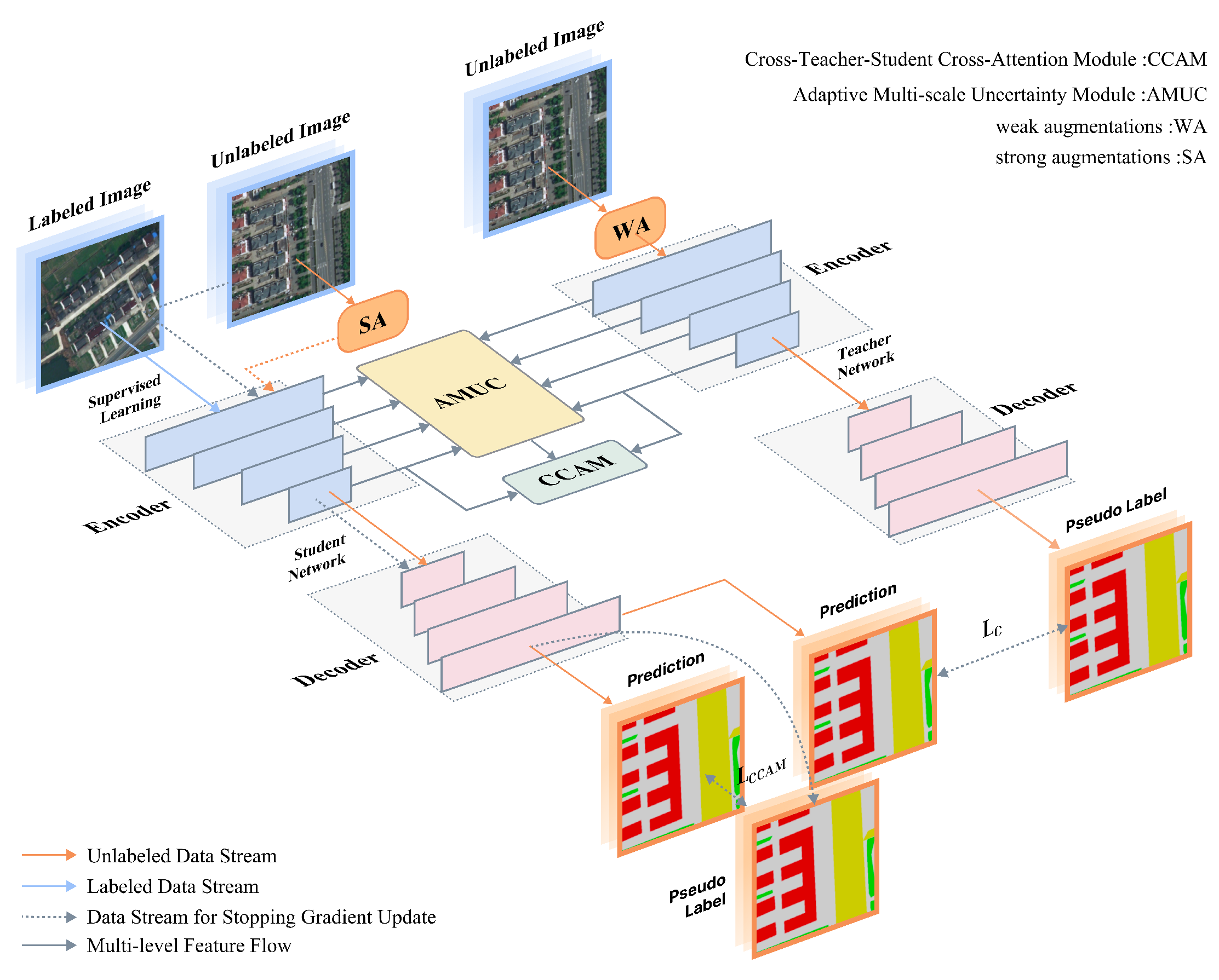
The overall architecture of MSCA-TSN is shown in Figure 1. The teacher branch receives weakly augmented inputs and provides relatively stable semantic guidance, whereas the student branch receives the corresponding strongly augmented inputs and learns to produce robust predictions under larger perturbations. AMUC is applied to hierarchical encoder features to estimate predictive uncertainty at multiple scales and to adaptively weight consistency constraints according to feature reliability. Meanwhile, CCAM performs cross-network attention interaction between student and teacher features, where student features generate queries and teacher features generate keys and values, thereby enabling the student branch to absorb stable class-aware contextual cues while preserving fine-grained details. The final prediction is optimized using supervised loss on labeled data together with multiple unsupervised objectives on unlabeled data.

3.1. Problem Definition

In semi-supervised RSI semantic segmentation, the training set is divided into a labeled subset and an unlabeled subset, denoted by

$$\mathcal{D}={\mathcal{D}}_L\cup {\mathcal{D}}_U,$$

(1)

where

$${\mathcal{D}}_L={\left\{(x_i^l,y_i)\right\}}_{i=1}^{N_L}, \hspace{1em}{\mathcal{D}}_U={\left\{x_i^u\right\}}_{i=1}^{N_U}.$$

(2)

Here, $x_i^l$ and $x_i^u$ denote labeled and unlabeled input images, respectively; $y_i$ is the ground-truth pixel-wise annotation corresponding to $x_i^l$; and $N_L$ and $N_U$ are the numbers of labeled and unlabeled samples.

Let $f_s(·)$ and $f_t(·)$ denote the student and teacher networks, respectively. For a labeled image $x_i^l$, the student network outputs a segmentation prediction $p_i^l=f_s\left(x_i^l\right)$. For an unlabeled image, weak and strong perturbations are applied to generate two correlated views, which are then fed into the teacher and student branches to construct consistency supervision. The overall optimization objective is defined as

$$L=L_S+L_U,$$

(3)

where $L_S$ is the supervised segmentation loss on labeled samples and $L_U$ is the unsupervised objective on unlabeled samples. The key challenge is therefore to design an unlabeled-data learning strategy that simultaneously improves boundary integrity, multi-scale robustness, and class discriminability.

3.2. Cross-Teacher–Student Cross-Attention Module

To alleviate the confusion between visually similar land-cover categories, we introduce the CCAM. The core idea is to explicitly construct cross-network attention between teacher and student features rather than performing self-attention within a single branch. In our design, the student features serve as queries, while the teacher features serve as keys and values. This formulation is consistent with the intended teacher–student interaction: the student branch retains stronger detail sensitivity under strong augmentation, whereas the teacher branch provides more stable semantic priors.

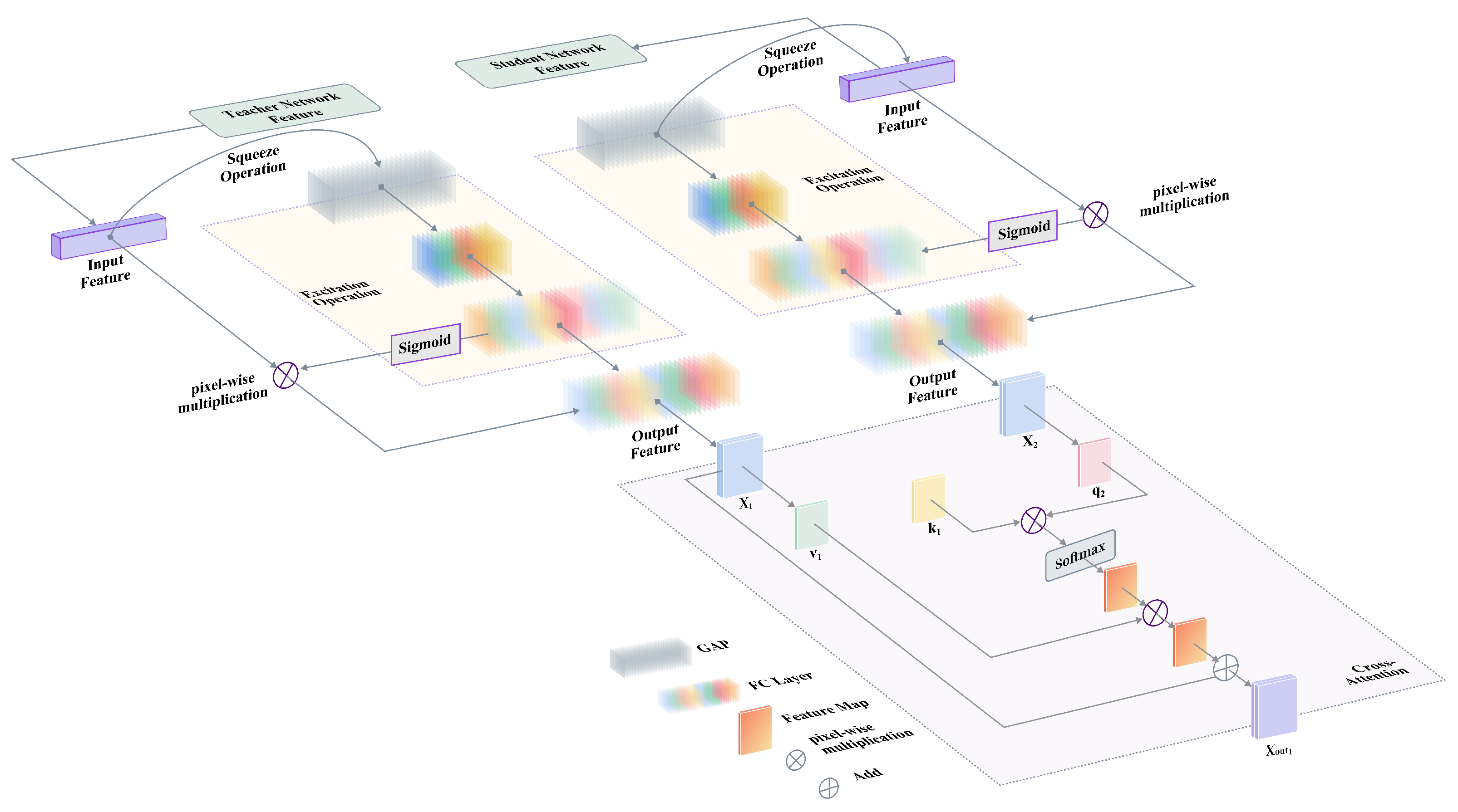
As illustrated in Figure 2, CCAM operates on the fourth-stage encoder features $F_4^s\in {\mathbb{R}}^{H_4\times W_4\times C}$ and $F_4^t\in {\mathbb{R}}^{H_4\times W_4\times C}$ from the student and teacher branches, respectively. We first apply channel attention to both feature maps in order to suppress noisy channels and strengthen informative spectral–spatial responses:

$${\widehat{F}}_4^s=\mathrm{ChannelAttn}\left(F_4^s\right),\hspace{1em} {\widehat{F}}_4^t=\mathrm{ChannelAttn}\left(F_4^t\right).$$

(4)

Here, $\mathrm{ChannelAttn}(·)$ denotes a channel reweighting operation implemented by global average pooling followed by a lightweight two-layer transformation and sigmoid normalization.

Figure 2. Overview of the revised CCAM. After channel refinement, student and teacher encoder features are flattened and linearly projected. The student branch generates the query matrix, whereas the teacher branch generates the key and value matrices. Cross-attention is then computed to transfer stable semantic cues from the teacher to the student, yielding a more discriminative fused representation for subsequent decoding.

Figure 2. Overview of the revised CCAM. After channel refinement, student and teacher encoder features are flattened and linearly projected. The student branch generates the query matrix, whereas the teacher branch generates the key and value matrices. Cross-attention is then computed to transfer stable semantic cues from the teacher to the student, yielding a more discriminative fused representation for subsequent decoding.

For clarity, Figure 2 can be interpreted in three steps: (i) channel refinement of the student and teacher features, (ii) cross-attention interaction between the two branches, and (iii) prediction supervision using the fused representation. After channel refinement, the two feature maps are flattened along the spatial dimension. Let $N=H_4{W}_4$ be the number of spatial positions. The flattened representations are written as

$$X_4^s=\mathrm{Flatten}({\widehat{F}}_4^s)\in {\mathbb{R}}^{N\times C},\hspace{1em} X_4^t=\mathrm{Flatten}({\widehat{F}}_4^t)\in {\mathbb{R}}^{N\times C}.$$

(5)

The query, key, and value matrices are then generated by linear projections:

$$Q=X_4^s{W}_Q,\hspace{1em} K=X_4^t{W}_K,\hspace{1em} V=X_4^t{W}_V,$$

(6)

where $W_Q\in {\mathbb{R}}^{C\times d}$, $W_K\in {\mathbb{R}}^{C\times d}$, and $W_V\in {\mathbb{R}}^{C\times d}$ are learnable projection matrices, and d is the latent attention dimension. It is worth emphasizing that only the student feature generates Q, while the teacher feature generates K and V, thereby forming genuine cross-attention.

The affinity matrix is computed as

$$A=\mathrm{Softmax}\left({\displaystyle \frac{\mathrm{\Psi }\left(Q{K}^{\top }\right)}{\sqrt{d}}}\right)\in {\mathbb{R}}^{N\times N},$$

(7)

where $\mathrm{\Psi }(·)$ denotes instance normalization applied to the similarity matrix to stabilize the scale of attention responses. Compared with the original expression, the revised formulation explicitly uses $Q{K}^{\top }$ rather than $Q^{\top }K$, which yields the correct spatial attention shape.

The attention-weighted output is obtained by

$$O=AV\in {\mathbb{R}}^{N\times d},$$

(8)

followed by a linear projection and spatial reshaping:

$$F_{\mathrm{out}}=\mathrm{Reshape}\left(O{W}_O\right)\in {\mathbb{R}}^{H_4\times W_4\times C},$$

(9)

where $W_O\in {\mathbb{R}}^{d\times C}$ is the output projection matrix. The fused feature $F_{\mathrm{out}}$ is then sent to the decoder to generate refined student predictions for unlabeled samples.

To supervise the CCAM-enhanced prediction on unlabeled data, we use the teacher prediction to generate pseudo-labels together with a confidence mask. Let ${\widehat{y}}_{i,j}$ denote the teacher-derived pseudo-label at pixel j of sample i, and let ${\mathcal{M}}_i$ denote the set of high-confidence pixels retained by the teacher branch. The CCAM loss is defined as

$$L_{CCAM}={\displaystyle \frac{1}{{\sum }_{i=1}^{N_U}\left|{\mathcal{M}}_i\right|}}\sum _{i=1}^{N_U}\sum _{j\in {\mathcal{M}}_i}{L}_{CE}\left(p_{i,j}^u,{\widehat{y}}_{i,j}\right),$$

(10)

where $p_{i,j}^u$ is the student prediction at the corresponding pixel and $L_{CE}(·,·)$ denotes the cross-entropy loss. This masked formulation ensures that CCAM is mainly guided by reliable teacher supervision rather than by noisy unlabeled pixels.

3.3. Adaptive Multi-Scale Uncertainty Consistency Module

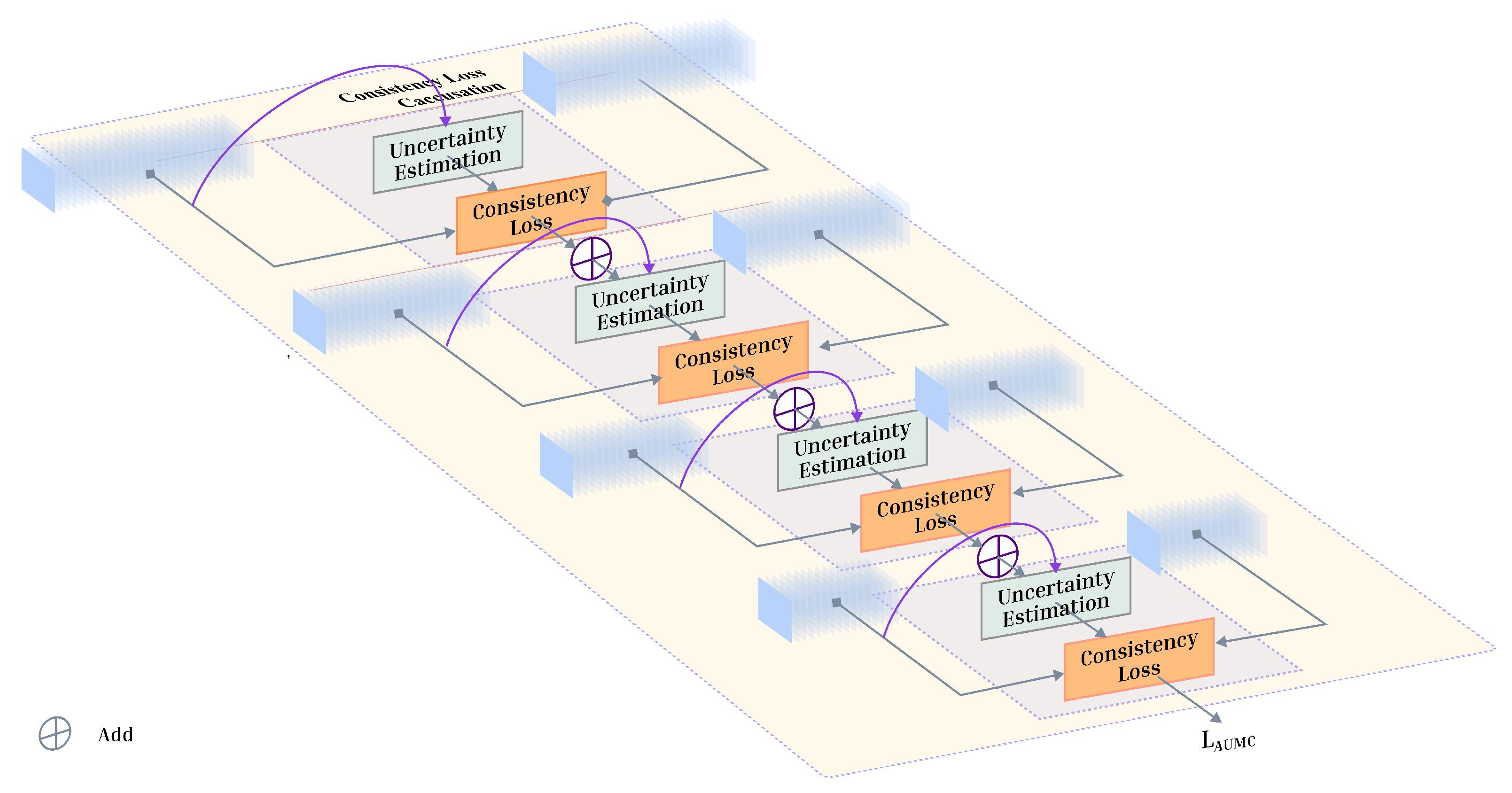
Most semi-supervised segmentation methods enforce consistency only at the final prediction layer, which is insufficient for RSIs containing substantial scale variation and ambiguous object boundaries. To better exploit hierarchical information, we design the AMCU, which imposes uncertainty-aware consistency constraints on multiple encoder stages. Its purpose is twofold: first, to identify which feature levels provide more reliable supervision; second, to restrict the consistency objective mainly to low-uncertainty spatial regions, thereby reducing error propagation from unstable features.

AMUC operates on four encoder levels, denoted by $F_k^s$ and $F_k^t$ for the student and teacher branches, respectively, where $k\in \{1,2,3,4\}$ corresponds from shallow to deep stages. Each feature map has size ${\mathbb{R}}^{H_k\times W_k\times C_k}$. As shown in Figure 3, the module contains three stages: predictive uncertainty estimation, adaptive weight generation, and weighted multi-scale consistency learning.

For uncertainty estimation, Monte Carlo Dropout (MCD) is activated on the teacher branch at each encoder level. For the k-th stage, we perform T stochastic forward passes and obtain a sequence of predictive probability tensors:

$$p_{k,t}=\mathrm{softmax}\left(g_k\left(F_{k,t}^t\right)\right),\hspace{1em} t=1,2,\dots ,T,$$

(11)

where $F_{k,t}^t$ is the teacher feature under the t-th stochastic dropout realization and $g_k(·)$ denotes the corresponding lightweight prediction head used for uncertainty estimation at stage k.

Different from the original formulation based on the average of entropies, we estimate uncertainty using the predictive entropy of the mean predictive distribution. Specifically, the mean predictive distribution is first computed as

$${\overline{p}}_k={\displaystyle \frac{1}{T}}\sum _{t=1}^T{p}_{k,t},$$

(12)

and the uncertainty map at the k-th feature level is then defined by

$$u_k=-\sum _{c=1}^C{\overline{p}}_k\left(c\right)log\left({\overline{p}}_k\left(c\right)\right),$$

(13)

where C is the number of semantic classes and $u_k$ is computed at each spatial position. A larger entropy indicates a less reliable prediction at that location.

After obtaining uncertainty maps at different feature levels, we assign an adaptive weight to each level according to its mean uncertainty:

$$w_k={\displaystyle \frac{exp\left(-\gamma \mathrm{Mean}\left(u_k\right)\right)}{{\sum }_{m=1}^{4}exp\left(-\gamma \mathrm{Mean}\left(u_m\right)\right)}},\hspace{1em} k=1,2,3,4,$$

(14)

where $\gamma$ is a temperature coefficient controlling the sharpness of the level-weight distribution. In this way, feature levels with lower average uncertainty are assigned larger weights, while unstable levels contribute less to the consistency objective.

To avoid enforcing consistency on unreliable regions, we define a low-uncertainty mask for each level as

$${\mathrm{\Omega }}_k=\left\{j\mid u_k\left(j\right)<\tau ·max\left(u_k\right)\right\},$$

(15)

where $\tau$ is the uncertainty threshold and j indexes the spatial positions of the k-th feature map. The Huber function is used because it is less sensitive to outliers than a pure ${\mathcal{\ell }}_2$ penalty:

$$\mathrm{Huber}(y,\widehat{y})=\left\{\begin{array}{cc}{\displaystyle \frac{1}{2}}{(y-\widehat{y})}^2,\hfill & \mathrm{if} |y - \widehat{y}| \le \delta ,\hfill \\ \delta \left(|y - \widehat{y}| - {\displaystyle \frac{1}{2}}\delta \right),\hfill & \mathrm{otherwise},\hfill \end{array}\right.$$

(16)

where $\delta$ is the transition point between the quadratic and linear regimes. In our implementation, the Huber penalty is applied element-wise and then averaged across channels.

The uncertainty-masked consistency loss at level k is written as

$$L_{\mathrm{consist}}^k={\displaystyle \frac{1}{|{\mathrm{\Omega }}_k|}}\sum _{j\in {\mathrm{\Omega }}_k}\mathrm{Huber}\left(F_{k,j}^s,\mathrm{sg}(F_{k,j}^t)\right),$$

(17)

where $\mathrm{sg}(·)$ denotes the stop-gradient operator applied to the teacher features. The final AMUC loss is the weighted sum of all hierarchical consistency terms:

$$L_{AMUC}=\sum _{k=1}^4{w}_k L_{\mathrm{consist}}^k.$$

(18)

3.4. Training Strategy and Hyperparameter Setting

To make the training process more explicit, we summarize the teacher–student optimization strategy here. For each unlabeled sample $x_i^u$, a weakly augmented view $x_i^{u,w}$ is fed into the teacher branch, while a strongly augmented view $x_i^{u,s}$ is fed into the student branch. The weak view is used to produce relatively stable pseudo supervision, whereas the strong view encourages the student network to learn perturbation-invariant representations. For labeled samples, the student branch is directly supervised by ground-truth annotations.

The teacher parameters are updated by exponential moving average (EMA) of the student parameters:

$${\theta }_t\leftarrow m {\theta }_t+(1-m) {\theta }_s,$$

(19)

where ${\theta }_t$ and ${\theta }_s$ denote the teacher and student parameters, respectively, and m is the EMA momentum coefficient. This update rule allows the teacher branch to provide smoother and more reliable supervision throughout training.

The main hyperparameters in AMUC are T, $\tau$, and $\gamma$. These three variables are selected for explicit analysis because they directly control the uncertainty modeling process: T determines the stability of Monte Carlo uncertainty estimation, $\tau$ controls the spatial range of low-uncertainty regions participating in consistency learning, and $\gamma$ regulates the contrast among hierarchical level weights. Following the parameter sensitivity analysis reported later, the default settings are $T=10$, $\tau =0.6$, and $\gamma =2.0$. By moving this training-related explanation into the Methods section, the manuscript more clearly connects the design of AMUC with the subsequent parameter study.

3.5. Loss Function

The overall objective contains one supervised term and three unsupervised terms. For labeled data, the supervised loss is defined as

$$L_S={\displaystyle \frac{1}{N_L}}\sum _{i=1}^{N_L}{L}_{CE}\left(p_i^l,y_i\right),$$

(20)

where $p_i^l$ denotes the student prediction for the labeled image $x_i^l$.

For unlabeled data, we use a basic teacher–student consistency term together with the proposed AMUC and CCAM terms. Let ${\tilde{y}}_{i,j}$ denote the teacher-derived pseudo-label at pixel j and let ${\mathcal{M}}_i$ be the corresponding confidence mask. The basic consistency loss is written as

$$L_C={\displaystyle \frac{1}{{\sum }_{i=1}^{N_U}\left|{\mathcal{M}}_i\right|}}\sum _{i=1}^{N_U}\sum _{j\in {\mathcal{M}}_i}{L}_{CE}\left(p_{i,j}^s,{\tilde{y}}_{i,j}\right),$$

(21)

where $p_{i,j}^s$ denotes the student prediction at the selected unlabeled pixel.

The total unsupervised loss is then given by

$$L_U=L_C+L_{AMUC}+L_{CCAM},$$

(22)

and the final training objective becomes

$$L=L_S+L_U.$$

(23)

This formulation makes the role of each component explicit: $L_C$ provides standard pseudo-label supervision, $L_{AMUC}$ enhances multi-scale reliability-aware consistency, and $L_{CCAM}$ strengthens cross-network discriminative representation learning.

4. Results

In this section, we first describe the experimental settings, including the dataset configuration and implementation details. We then compare the proposed MSCA-TSN with several representative semi-supervised segmentation approaches. The results show that MSCA-TSN achieves superior performance. Finally, ablation studies are conducted to validate the effectiveness of the AMUC and the CCAM.

4.1. Experimental Settings

4.1.1. Datasets

To comprehensively evaluate the effectiveness of the proposed method under limited-label remote sensing scenarios, experiments are conducted on two widely used high-resolution remote sensing datasets, namely LoveDA [63] and ISPRS Potsdam [64]. These two benchmarks differ in scene characteristics, object scales, and spatial resolutions and therefore provide a suitable test bed for assessing both multi-scale modeling capability and boundary delineation quality.

In our experiments, we conduct extensive evaluations on two challenging high-resolution remote sensing datasets, namely LoveDA [63] and ISPRS Potsdam [64]. The LoveDA dataset contains 5987 high-resolution RSIs from three cities, with a spatial resolution of 0.3 m and a size of $1024\times 1024$ pixels. It provides 166,768 annotated instances covering seven land-cover categories: building, road, water, barren land, forest, farmland, and background. Owing to its large intra-class scale variation, complex background interference, and frequent boundary ambiguity among adjacent categories, LoveDA is particularly suitable for evaluating semi-supervised segmentation methods under challenging real-world conditions. The LoveDA dataset is split into training, validation, and test sets with a ratio of 6:2:2, where the training set includes 2522 fully annotated images. All original images are cropped into non-overlapping $512\times 512$ patches. For the semi-supervised setting, we further divide the training set into labeled and unlabeled subsets with two representative labeling ratios, 5% and 10%, to evaluate the model generalization under limited annotations. Detailed statistics are summarized in

Table 1. Sample split of LoveDA dataset.

Dataset	Label Ratio	Labeled Training Set	Unlabeled Training Set	Validation Set	Test Set
LoveDA Dataset	5%	504	9584	3338	3338
	10%	1008	9080	3338	3338

.

In addition, the ISPRS Potsdam dataset consists of 38 aerial images over Potsdam, Germany, with dense pixel-level annotations. Each image has a size of $6000\times 6000$ pixels and an ultra-high spatial resolution of 0.05 m, covering six semantic classes: impervious surfaces, building, low vegetation, tree, car, and clutter/background. This dataset exhibits complex urban scenes with large building clusters, complicated road networks, and numerous small objects, which is suitable for testing the model robustness on fine-grained details and ambiguous boundaries. Compared with LoveDA, Potsdam places stronger emphasis on fine structural details and small-object recognition and is therefore useful for further validating the generalization of the proposed method across different remote sensing scene distributions. In our implementation, all original images are uniformly cropped into non-overlapping $512\times 512$ sub-images to meet the network input requirement.

4.1.2. Experimental Details

All experiments are conducted on an Ubuntu 18.04.6 operating system equipped with an NVIDIA A40 GPU (48 GB memory). The deep learning framework is PyTorch 1.11.0, with Python 3.8.15 adopted for code implementation. To quantitatively assess segmentation performance from both region-level and boundary-level perspectives, four evaluation metrics are considered, including mean Intersection over Union (mIoU), mean F1-score (mF1), Cohen’s Kappa coefficient (Kappa), and boundary F1 score (BF score). Among them, mIoU, mF1, and Kappa are standard region-based metrics widely adopted in semantic segmentation, whereas BF score is additionally introduced to better evaluate boundary localization quality, which is particularly relevant to the objectives of this work. Their calculation formulas are defined as follows:

$$\mathrm{mIoU}={\displaystyle \frac{1}{C}}\sum _{i=0}^{C-1}{\displaystyle \frac{T{P}_i}{T{P}_i+F{P}_i+F{N}_i}}$$

(24)

$$\mathrm{mF}1={\displaystyle \frac{1}{C}}\sum _{i=0}^{C-1}{\displaystyle \frac{2\times T{P}_i}{2\times T{P}_i+F{P}_i+F{N}_i}}$$

(25)

$$\mathrm{Kappa}={\displaystyle \frac{p_0-p_e}{1-p_e}}$$

(26)

where $p_0={\displaystyle \frac{1}{N}}{\sum }_{i=0}^{C-1}T{P}_i$ and $p_e={\displaystyle \frac{1}{N^2}}{\sum }_{i=0}^{C-1}(T{P}_i+F{N}_i)(T{P}_i+F{P}_i)$.

For boundary evaluation, the BF score is defined as

$$P_b={\displaystyle \frac{T{P}_b}{T{P}_b+F{P}_b}},$$

(27)

$$R_b={\displaystyle \frac{T{P}_b}{T{P}_b+F{N}_b}},$$

(28)

$$\mathrm{BF}={\displaystyle \frac{2\times P_b\times R_b}{P_b+R_b}},$$

(29)

where $T{P}_b$, $F{P}_b$, and $F{N}_b$ denote the correctly matched, falsely predicted, and missed boundary pixels, respectively. A higher BF score indicates better alignment between predicted and reference boundaries.

In the above formulas, C denotes the number of semantic categories, $T{P}_i$ represents the number of true positive pixels for the i-th category, $F{P}_i$ is the number of false positive pixels, $F{N}_i$ is the number of false negative pixels, and N is the total number of pixels in the test set. Region-based metrics are used to evaluate overall semantic consistency, while the BF score provides complementary evidence on boundary preservation performance. Detailed configurations of hyperparameters are summarized in

Table 2. Hyperparameter settings.

Hyperparameter	Value
Batch Size	16
Optimizer	SGD
Initial Learning Rate	0.007
Maximum Iterations	200
Momentum	0.9
Weight Decay	0.0001
Image Size	$512\times 512$ Pixels

.

4.2. Comparison with Other Methods

To comprehensively evaluate the effectiveness of the proposed MSCA-TSN, we compare it with several representative semi-supervised segmentation methods on the LoveDA and ISPRS Potsdam datasets under limited-label settings. In addition to the region-based metrics, i.e., mIoU, mF1, and Kappa, we further report the boundary F1 score (BF score) to provide complementary quantitative evidence on boundary localization quality. Since the proposed method is specifically designed to improve multi-scale consistency and boundary integrity in remote sensing scenes, BF score helps better characterize its performance on thin structures, ambiguous edges, and fine-grained object contours.

4.2.1. Results on LoveDA Dataset

As shown in

Table 3. Comparison on the LoveDA dataset. Bold indicates the best result.

Label Ratio	Method	IoU Metrics (%)								Metrics
		Background	Building	Road	Water	Barren Land	Forest	Farmland		mIoU (%)	mF1 (%)	Kappa	BF
5%	Mean Teacher [41]	49.73	46.22	42.34	60.93	31.51	35.79	44.22		44.39	61.81	0.5151	59.42
	FixMatch [49]	45.40	53.05	51.22	66.73	28.53	27.25	54.30		44.64	62.45	0.5378	60.18
	CPS [50]	48.90	49.64	47.97	60.27	4.67	36.09	47.32		42.12	56.90	0.4976	55.03
	LSST [65]	51.48	45.66	52.66	67.63	33.52	35.80	48.60		47.91	64.10	0.5434	61.52
	U2PL [66]	52.58	53.12	50.97	65.75	16.48	38.16	47.89		46.42	61.93	0.5391	59.86
	CCVC [67]	44.17	42.82	35.09	51.20	3.17	31.40	44.62		36.07	50.93	0.4397	48.71
	UniMatch [51]	50.20	54.49	50.46	67.18	26.79	30.06	54.86		47.72	63.46	0.5543	61.89
	AllSpark [17]	65.09	55.06	47.59	67.10	34.67	26.86	51.87		49.75	64.91	0.5682	62.47
	DWL [61]	48.75	55.00	51.53	69.49	29.46	36.59	52.11		48.99	64.88	0.5597	63.02
	MSCA-TSN	52.00	62.22	51.99	71.13	24.44	37.43	58.13		51.05	66.28	0.6150	65.21
10%	Mean Teacher [41]	50.45	55.75	43.56	66.15	35.24	36.96	45.64		47.68	64.18	0.5387	61.33
	FixMatch [49]	51.02	54.59	52.20	56.91	24.86	39.83	56.50		47.99	64.97	0.5676	62.04
	CPS [50]	51.30	54.93	52.57	53.37	18.39	37.59	53.24		45.91	61.78	0.5479	57.46
	LSST [65]	50.69	49.50	52.63	69.85	27.25	36.24	52.06		48.32	64.17	0.5565	62.11
	U2PL [66]	51.44	53.44	53.43	56.82	29.44	39.55	51.89		48.00	64.32	0.5537	61.68
	CCVC [67]	46.79	40.25	46.96	45.79	19.57	26.58	38.38		37.76	54.01	0.4389	50.72
	UniMatch [51]	51.80	53.95	51.17	58.15	25.60	38.72	54.86		47.75	63.86	0.5639	62.27
	AllSpark [17]	67.13	56.16	40.67	63.58	32.54	32.03	56.91		49.86	63.97	0.5751	63.15
	DWL [61]	49.94	56.66	53.89	70.35	30.62	41.49	53.13		50.87	66.64	0.5753	64.28
	MSCA-TSN	50.77	61.58	55.17	71.66	29.94	37.93	59.82		52.41	67.73	0.6257	66.41

, MSCA-TSN achieves the best overall performance on the LoveDA dataset under both 5% and 10% labeling ratios. At the 5% labeling ratio, MSCA-TSN obtains 51.05% mIoU, 66.28% mF1, 0.6150 Kappa, and 65.21 BF, outperforming the second-best method AllSpark by 1.30 points in mIoU and 2.74 points in BF. When the labeling ratio increases to 10%, the proposed method further improves to 52.41% mIoU, 67.73% mF1, 0.6257 Kappa, and 66.41 BF, remaining the top-performing method across all four overall metrics. These results indicate that the proposed framework improves not only region-level semantic prediction but also boundary alignment quality under limited supervision.

From the class-wise IoU comparison, MSCA-TSN shows clear advantages on categories closely related to geometric completeness and boundary continuity, especially building, road, water, and farmland. At the 5% labeling ratio, it achieves the highest IoU values on building (62.22%), road (51.99%), water (71.13%), and farmland (58.13%). At the 10% labeling ratio, the same trend remains, with MSCA-TSN achieving the best IoU values on building (61.58%), road (55.17%), water (71.66%), and farmland (59.82%). These categories are frequently affected by elongated boundaries, fine structures, and confusing adjacent classes in LoveDA, which suggests that the uncertainty-aware multi-scale consistency and cross-network attention interaction are beneficial for preserving structurally meaningful regions.

Compared with other methods, the proposed method also exhibits stronger overall balance across categories. For example, AllSpark achieves competitive overall performance and obtains higher background IoU in both settings, while DWL and U²PL perform well on individual categories such as forest. However, MSCA-TSN consistently delivers the best overall mIoU and BF score, indicating that its advantage is not limited to one or two classes but is reflected in more reliable holistic segmentation. It is also worth noting that MSCA-TSN is not the best on every single class, such as barren land or forest in some settings. Nevertheless, its more favorable overall metric combination demonstrates a better trade-off between semantic consistency and boundary quality in complex remote sensing scenes.

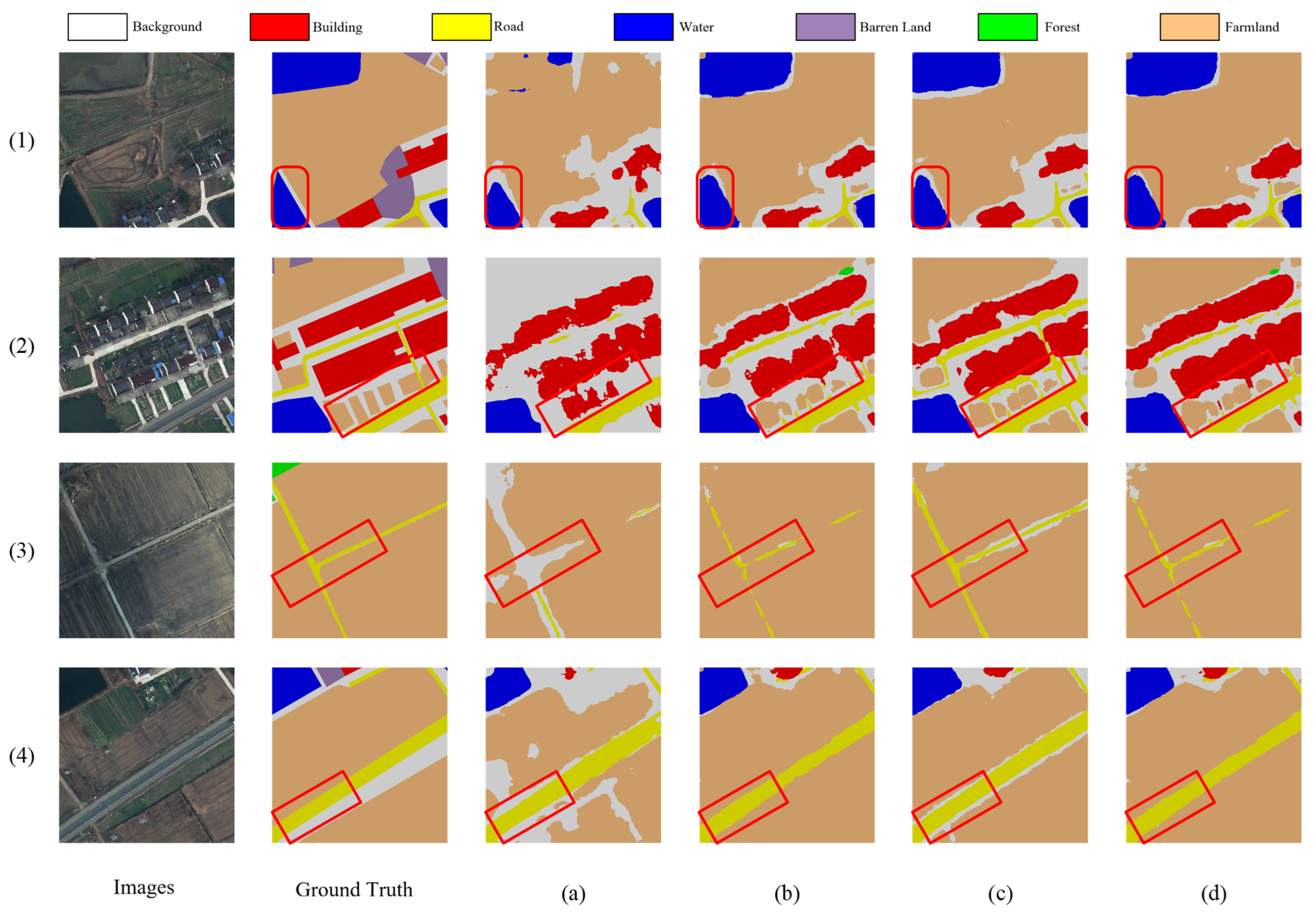
Figure 4 provides qualitative comparisons on LoveDA at the 10% labeling ratio. The red boxes highlight representative regions with ambiguous boundaries, narrow road structures, and confusing adjacent classes. In region (1), Mean Teacher, FixMatch, and CPS show noticeable distortions around the water–farmland transition and the local corner boundary, whereas MSCA-TSN preserves a cleaner and more coherent contour. In region (2), the proposed method produces more regular building shapes and clearer separation between roads, buildings, and farmland, while the comparison methods introduce fragmented predictions or local category leakage. In regions (3) and (4), which mainly contain thin road structures embedded in farmland, MSCA-TSN maintains better road continuity and boundary sharpness. These qualitative observations are consistent with the higher BF scores reported in Table 3, suggesting that the proposed method is more effective in handling boundary-sensitive structures in complex rural scenes.

4.2.2. Results on ISPRS Potsdam Dataset

As shown in

Table 4. Quantitative comparison on the ISPRS Potsdam dataset. Bold indicates the best result.

Label Ratio	Method	IoU Metrics (%)						Metrics
		Building	Low Veg.	Tree	Car	Imp. Surfaces		mIoU (%)	mF1 (%)	Kappa	BF
5%	Mean teacher [41]	82.15	65.92	67.11	72.21	74.60		72.40	83.86	0.7403	82.64
	CutMix [44]	52.94	68.86	41.51	58.33	54.82		55.29	70.79	0.5783	68.95
	CCT [48]	72.90	80.25	64.23	58.32	74.42		70.02	82.12	0.7236	80.46
	CPS [50]	76.53	84.34	57.98	69.45	75.39		72.74	83.78	0.7492	82.31
	LSST [65]	69.26	84.55	67.33	67.49	73.86		72.50	83.67	0.7399	82.18
	FixMatch [49]	78.12	74.87	68.89	66.58	75.30		72.75	84.15	0.7497	82.74
	UniMatch [51]	78.24	73.59	67.17	66.64	75.07		72.14	83.73	0.7432	82.26
	DWL [61]	74.81	85.64	63.68	62.99	75.68		73.10	84.22	0.7507	82.87
	AllSpark [17]	85.57	67.62	60.61	73.48	77.15		72.88	84.04	0.7989	83.22
	MUCA [30]	88.45	69.53	61.39	74.18	79.56		74.62	85.15	0.8166	84.36
	MSCA-TSN	89.12	70.25	62.18	75.05	80.15		75.35	85.88	0.8258	85.17
10%	Mean teacher [41]	84.76	69.28	68.83	71.66	76.51		74.21	85.07	0.7578	83.78
	CutMix [44]	64.55	80.99	64.79	65.50	68.01		68.77	81.34	0.7109	79.63
	CCT [48]	73.09	83.94	61.12	60.45	73.06		70.33	82.27	0.7265	80.72
	CPS [50]	77.80	87.15	61.12	68.48	75.89		74.09	84.55	0.7533	82.97
	LSST [65]	70.92	86.06	68.91	70.22	74.89		74.20	84.95	0.7549	83.46
	FixMatch [49]	77.97	76.17	70.09	70.97	76.14		74.27	85.20	0.7606	83.71
	UniMatch [51]	77.34	87.75	70.79	56.65	76.46		73.80	84.52	0.7599	83.02
	DWL [61]	76.37	88.42	66.54	64.37	77.14		74.57	85.16	0.7628	83.95
	AllSpark [17]	86.29	69.83	64.17	75.23	78.31		74.76	85.35	0.8144	84.47
	MUCA [30]	88.02	70.58	64.53	75.20	79.92		75.65	85.90	0.8245	85.08
	MSCA-TSN	89.05	71.12	65.08	75.88	80.56		76.34	86.52	0.8325	85.89

, MSCA-TSN also achieves the best overall performance on the ISPRS Potsdam dataset under both labeling ratios. At the 5% labeling ratio, it obtains 75.35% mIoU, 85.88% mF1, 0.8258 Kappa, and 85.17 BF, outperforming the second-best method MUCA by 0.73 points in mIoU and 0.81 points in BF. At the 10% labeling ratio, MSCA-TSN further improves to 76.34% mIoU, 86.52% mF1, 0.8325 Kappa, and 85.89 BF, again ranking first across all overall metrics. This indicates that the proposed framework remains effective not only on mixed rural-urban scenes such as LoveDA but also on ultra-high-resolution urban aerial imagery with more fine-grained structural details.

At the category level, MSCA-TSN shows particularly strong performance on building, car, and impervious surfaces, which are important classes for urban remote sensing analysis and are also highly sensitive to structural continuity and local boundary precision. At the 5% labeling ratio, it achieves the highest IoU values on building (89.12%), car (75.05%), and impervious surfaces (80.15%). At the 10% labeling ratio, the same trend is preserved, with the best IoU values on building (89.05%), car (75.88%), and impervious surfaces (80.56%). Although some competing methods perform better on individual classes such as low vegetation or tree, MSCA-TSN provides the most favorable overall trade-off across semantic regions and boundary quality, as reflected by its highest mIoU, mF1, Kappa, and BF score.

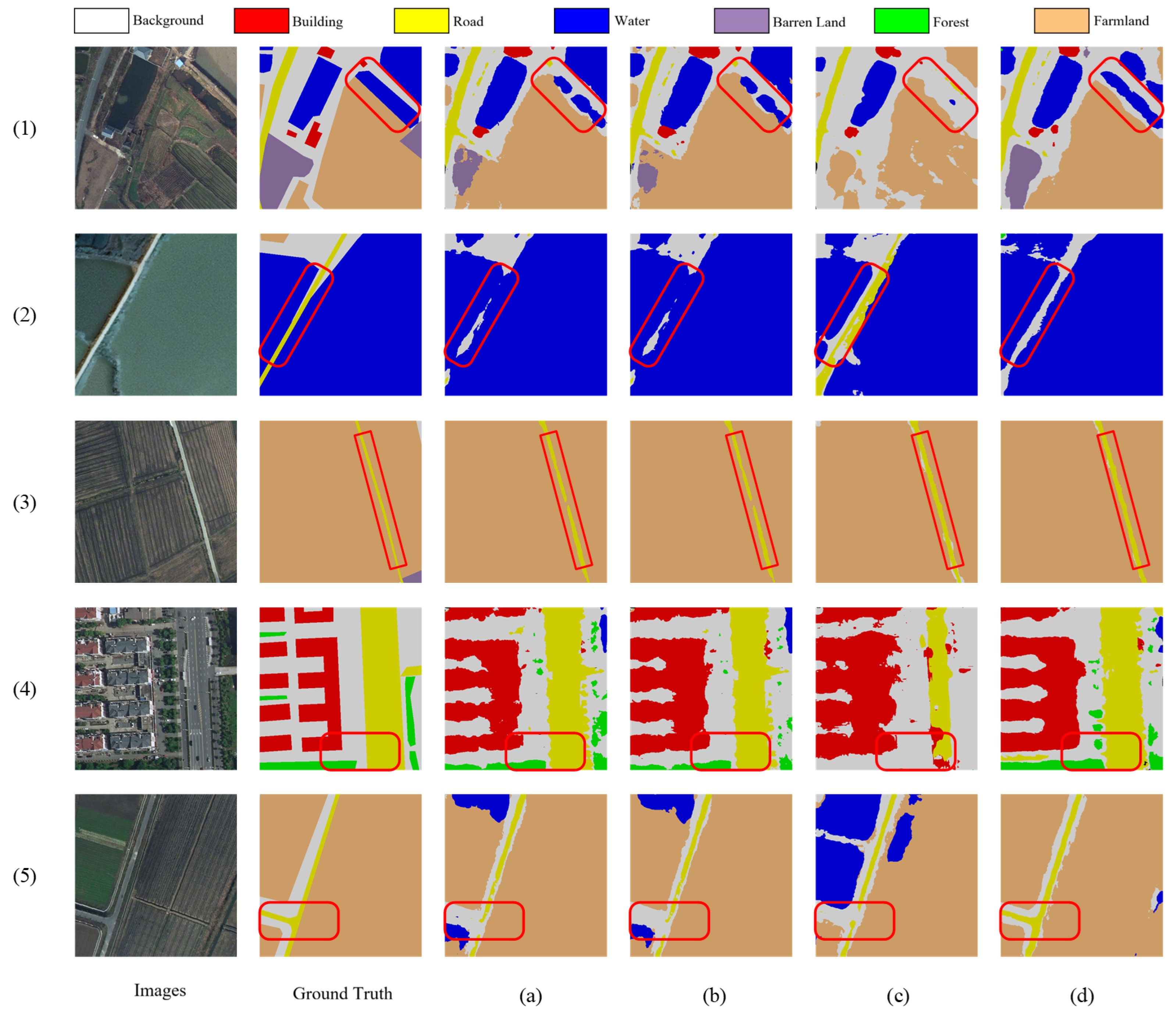
It is also worth noting that the closest remote sensing-specific comparison, MUCA, already performs strongly on Potsdam. Nevertheless, MSCA-TSN still achieves consistent gains over MUCA on both overall metrics and BF score. This suggests that the revised uncertainty-aware hierarchical consistency design and the clarified cross-network attention interaction provide additional benefits for fine structure recovery and boundary-preserving segmentation. Compared with AllSpark, which is a Transformer-based architecture-level method, the proposed model also delivers stronger results in this RSI-specific limited-label setting, indicating that the current design is well aligned with the characteristics of high-resolution RSI.

Figure 5 shows representative visualization results on the Potsdam dataset with the 10% labeling ratio. The highlighted regions indicate several typical challenges in ultra-high-resolution urban scenes, including narrow linear structures, water–road boundaries, and fragmented small-object regions. In regions (1), (2), and (5), MSCA-TSN produces cleaner and more stable boundaries around the elongated water and road structures, whereas the comparison methods introduce local boundary breaks, over-smoothing, or semantic leakage. In region (3), the proposed method better preserves the continuity of the thin road-like structure embedded in farmland. In region (4), MSCA-TSN yields a more coherent separation among road, building, and surrounding small fragmented regions, reflecting stronger robustness in mixed urban details. These observations agree well with the higher BF score reported in Table 4, further supporting the boundary-preserving capability of the proposed method.

4.3. Ablation Study

To validate the individual and joint contributions of the proposed modules, ablation experiments are conducted on the LoveDA dataset under the 10% labeling ratio, which is a representative and challenging semi-supervised setting used throughout this study. Quantitative results are reported in

Table 5. Ablation results of different module configurations on the LoveDA dataset with 10% labeled data. Bold indicates the best result.

Method	Modules			IoU Metrics (%)								Metrics
	AMUC	CCAM		Background	Building	Road	Water	Barren Land	Forest	Farmland		mIoU (%)	mF1 (%)	Kappa	BF
MSCA-TSN				48.00	43.34	50.56	61.42	23.14	37.63	45.00		$44.16\pm 0.28$	$60.46\pm 0.31$	$0.5061\pm 0.0042$	$58.92\pm 0.34$
	✓			50.31	57.03	42.86	69.11	25.03	40.32	59.02		$49.10\pm 0.24$	$64.74\pm 0.27$	$0.5989\pm 0.0035$	$63.10\pm 0.29$
		✓		51.00	62.08	50.99	71.13	24.68	36.43	58.83		$50.73\pm 0.21$	$65.88\pm 0.25$	$0.6050\pm 0.0031$	$64.27\pm 0.27$
	✓	✓		50.77	61.58	55.17	71.66	29.94	37.93	59.82		$\mathbf{52.41}\pm \mathbf{0.17}$	$\mathbf{67.73}\pm \mathbf{0.22}$	$\mathbf{0.6257}\pm \mathbf{0.0026}$	$\mathbf{66.41}\pm \mathbf{0.25}$

, and qualitative comparisons are provided in Figure 6. In addition to mIoU, mF1, Kappa, and BF score, we further report the mean ± standard deviation of the overall metrics to reflect the stability of different module configurations across repeated runs.

As shown in Table 5, the baseline model without AMUC and CCAM achieves $44.16\pm 0.28$% mIoU, $60.46\pm 0.31$% mF1, $0.5061\pm 0.0042$ Kappa, and $58.92\pm 0.34$ BF. When both modules are enabled, the complete MSCA-TSN improves these metrics to $52.41\pm 0.17$%, $67.73\pm 0.22$%, $0.6257\pm 0.0026$, and $66.41\pm 0.25$, respectively. This corresponds to gains of 8.25 points in mIoU, 7.27 points in mF1, 0.1196 in Kappa, and 7.49 points in BF, indicating that the proposed design improves both region-level segmentation quality and boundary preservation. Moreover, the relatively smaller standard deviations of the full model suggest that the joint use of AMUC and CCAM also leads to more stable optimization behavior.

Introducing the AMUC module alone increases mIoU from 44.16% to 49.10%, mF1 from 60.46% to 64.74%, Kappa from 0.5061 to 0.5989, and BF from 58.92 to 63.10. The most notable gains are observed on building, water, and farmland, whose IoUs rise from 43.34%, 61.42%, and 45.00% to 57.03%, 69.11%, and 59.02%, respectively. These results suggest that uncertainty-aware multi-scale consistency is particularly helpful for categories with large structural extent or evident scale variation. It is worth noting that the road IoU decreases when only AMUC is used, implying that reliability screening alone may be insufficient for preserving thin elongated structures without additional discriminative interaction.

When the CCAM module is introduced alone, the model attains 50.73% mIoU, 65.88% mF1, 0.6050 Kappa, and 64.27 BF, all of which are higher than the baseline. In particular, building IoU increases by 18.74 points and water IoU increases by 9.71 points, indicating that cross-network attention effectively enhances feature discriminability for categories with regular geometry and clear semantic priors. Compared with AMUC alone, CCAM yields a larger overall gain in mIoU and BF, which suggests that explicit teacher–student feature interaction plays an important role in suppressing inter-class confusion.

When AMUC and CCAM are used jointly, the model achieves the best results on all overall metrics. In addition to improving building and water segmentation, the joint configuration raises road IoU to 55.17%, which is higher than both the AMUC-only and CCAM-only settings. This observation indicates a complementary effect between the two modules: AMUC provides more reliable hierarchical supervision, while CCAM enhances discriminative representation learning. Their combination is therefore more effective for preserving structural continuity and reducing boundary ambiguity in complex remote sensing scenes.

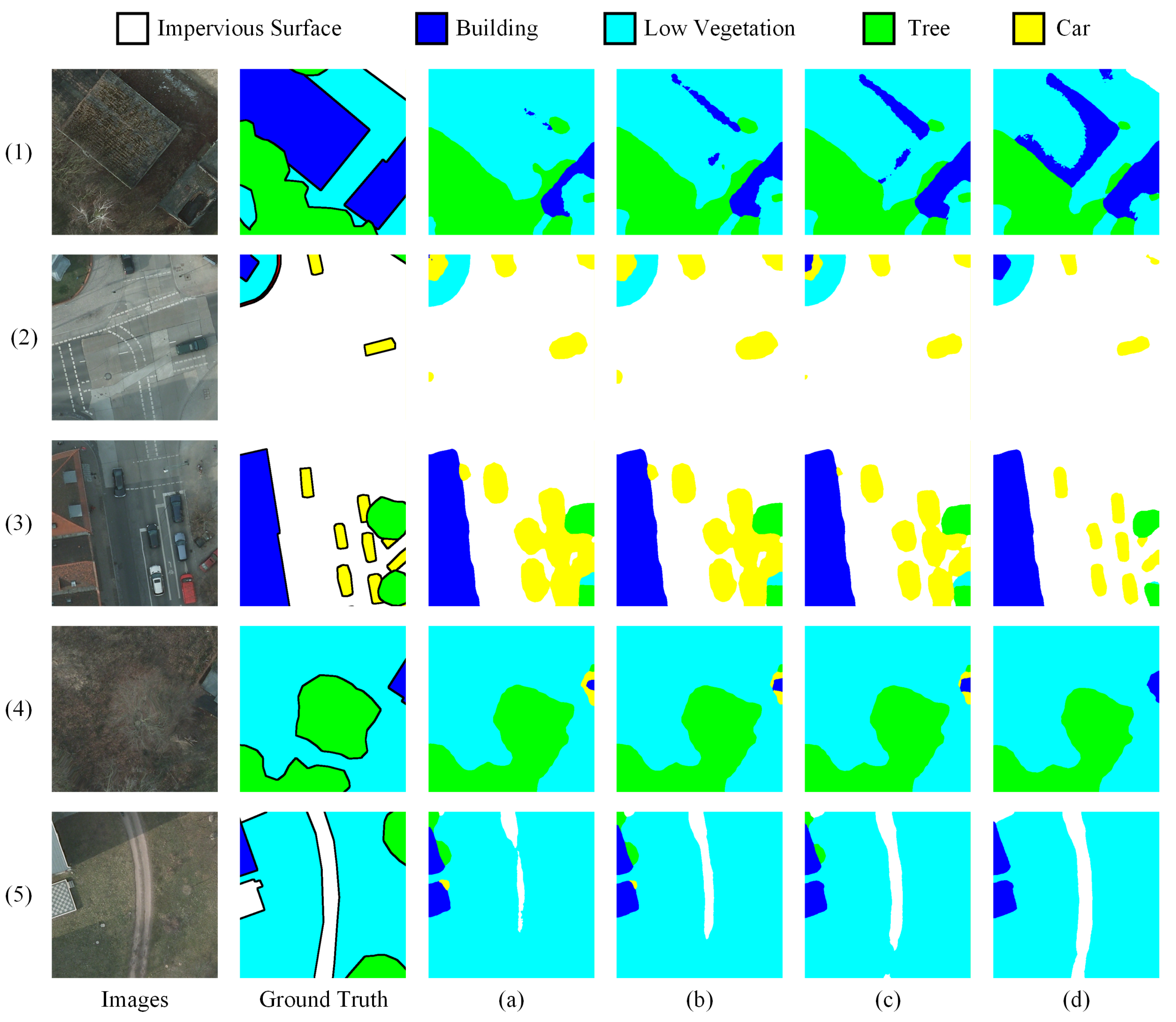
Figure 6 provides qualitative evidence that complements the quantitative results in Table 5. In the baseline setting shown in column (a), the segmentation results exhibit noticeable boundary distortion, local fragmentation, and incomplete structures. This is particularly evident in rows (1) and (4), where the water–farmland boundary and the elongated road region are both affected by obvious leakage and shape inconsistency.

After introducing AMUC only, as shown in column (b), the model produces more stable regional predictions on large homogeneous areas and better preserves the overall shapes of water bodies, farmland parcels, and buildings. For example, in row (1), the water boundary becomes more regular, and in row (2), the large building and farmland regions are segmented more coherently. However, some thin structures remain difficult to capture, which is consistent with the reduced road IoU in Table 5.

When only CCAM is enabled, as shown in column (c), the model shows stronger discriminative capability around ambiguous interfaces. In rows (2)–(4), the boundaries between buildings, roads, and surrounding land-cover classes become clearer, and the narrow road-like structures are better preserved than in the baseline setting. This observation agrees with the larger quantitative gains brought by CCAM on mIoU and BF score.

The complete model in column (d) achieves the most satisfactory visual performance. Compared with the other configurations, it preserves cleaner water contours in row (1), more regular building and farmland boundaries in row (2), better continuity of thin road structures in row (3), and more accurate alignment of elongated roads in row (4). These qualitative observations are consistent with the superior results of the full model on both region-based and boundary-based metrics, further supporting the complementary roles of AMUC and CCAM.

4.4. Parameter Sensitivity Analysis

To further evaluate the robustness of the proposed MSCA-TSN and to clarify the effects of the key hyperparameters in the AMCU, we conduct parameter sensitivity experiments on the LoveDA and ISPRS Potsdam datasets. The three analyzed parameters, namely the uncertainty threshold $\tau$, the temperature coefficient $\gamma$, and the number of Monte Carlo Dropout sampling passes T, are selected because they directly control the three core processes of AMUC: low-uncertainty region screening, adaptive weighting sharpness across hierarchical feature levels, and the stability of uncertainty estimation, respectively. Following the experimental settings in the previous sections, two semi-supervised scenarios with 5% and 10% labeling ratios are considered. In each experiment, only one parameter is varied while the others remain fixed to the default configuration. The segmentation performance is evaluated using mIoU (%), since it provides a concise and representative measure of the overall segmentation quality.

4.4.1. Sensitivity Analysis of the Uncertainty Threshold $\tau$

The uncertainty threshold $\tau$ determines the low-uncertainty pixel set involved in the multi-scale consistency constraint. When $\tau$ is small, only highly confident pixels participate in the consistency loss, which reduces the impact of noisy supervision but may lead to insufficient utilization of unlabeled data. Conversely, when $\tau$ is too large, more pixels are included in the consistency constraint, but unreliable boundary pixels may also be introduced, resulting in degraded supervision quality. Therefore, $\tau$ directly controls the trade-off between supervision reliability and effective pixel coverage. To investigate this effect, $\tau$ is varied from 0.4 to 0.8 while other hyperparameters remain fixed.

The quantitative results are summarized in

Table 6. Sensitivity analysis of the uncertainty threshold $\tau$ in AMUC in terms of mIoU (%). The bold text indicates the best results.

$\mathit{\tau }$	LoveDA		ISPRS Potsdam
	5% Label	10% Label	5% Label	10% Label
0.4	50.21	51.63	74.48	75.36
0.5	50.79	52.12	75.01	75.89
0.6	51.05	52.41	75.35	76.34
0.7	50.87	52.26	75.16	76.12
0.8	50.33	51.78	74.72	75.61

. It can be observed that the proposed MSCA-TSN achieves the best performance when $\tau =0.6$ across both datasets and labeling ratios. Specifically, the model obtains mIoU values of 51.05% and 52.41% on the LoveDA dataset under 5% and 10% labeling ratios, respectively, and 75.35% and 76.34% on the Potsdam dataset. When $\tau$ is smaller than 0.6, the model relies on a limited set of highly confident pixels and cannot fully exploit the unlabeled data. When $\tau$ becomes larger than 0.6, unreliable pixels gradually participate in the consistency loss, which slightly degrades segmentation performance. This phenomenon is consistent across both datasets, indicating that an overly conservative or overly loose uncertainty filter is suboptimal for semi-supervised RSI segmentation. Overall, the results indicate that a moderate uncertainty threshold provides the best balance between reliable supervision and sufficient pixel coverage.

4.4.2. Sensitivity Analysis of the Temperature Coefficient $\gamma$

The temperature coefficient $\gamma$ controls the sharpness of the adaptive weighting mechanism in AMUC. A small $\gamma$ leads to nearly uniform weights across different feature levels, which weakens the uncertainty-aware feature selection mechanism. In contrast, a very large $\gamma$ overly emphasizes a small number of low-uncertainty levels and suppresses the contribution of other feature levels, thereby reducing multi-scale complementarity. In other words, $\gamma$ determines how strongly the model differentiates reliable feature levels from relatively uncertain ones.

To analyze the influence of this parameter, $\gamma$ is varied from 0.5 to 4.0 while keeping the other hyperparameters fixed. The results are shown in

Table 7. Sensitivity analysis of the temperature coefficient $\gamma$ in AMUC in terms of mIoU (%). The bold text indicates the best results.

$\mathit{\gamma }$	LoveDA		ISPRS Potsdam
	5% Label	10% Label	5% Label	10% Label
0.5	50.31	51.84	74.83	75.77
1.0	50.76	52.19	75.17	76.05
2.0	51.05	52.41	75.35	76.34
3.0	50.91	52.28	75.12	76.18
4.0	50.58	51.96	74.89	75.94

. As $\gamma$ increases from 0.5 to 2.0, the segmentation performance gradually improves, indicating that uncertainty-aware weighting effectively enhances the contribution of reliable feature levels. When $\gamma$ exceeds 2.0, the performance begins to slightly decrease, suggesting that overly strong weighting reduces the contribution of complementary feature representations. The best overall results are achieved when $\gamma =2.0$, which validates the rationality of the default parameter setting adopted in this study. These results suggest that moderate feature-level selectivity is more beneficial than either nearly uniform weighting or excessively concentrated weighting.

4.4.3. Sensitivity Analysis of the Number of Monte Carlo Dropout Passes T

The number of Monte Carlo Dropout sampling passes T determines the stability of uncertainty estimation in AMUC. A small T may lead to unstable uncertainty estimation, which affects the reliability of uncertainty-aware consistency learning. Increasing T improves the stability of uncertainty estimation but also increases computational cost. Therefore, T is a parameter that directly reflects the trade-off between estimation reliability and computational efficiency.

To evaluate this trade-off, we vary T from 2 to 10 while keeping the remaining hyperparameters unchanged. The results are reported in

Table 8. Sensitivity analysis of the number of Monte Carlo Dropout passes T in terms of mIoU (%). The bold text indicates the best results.

T	LoveDA		ISPRS Potsdam
	5% Label	10% Label	5% Label	10% Label
2	49.88	51.37	74.46	75.31
4	50.36	51.82	74.87	75.79
6	50.72	52.11	75.08	76.02
8	50.96	52.32	75.27	76.22
10	51.05	52.41	75.35	76.34

. It can be observed that the segmentation performance improves gradually as T increases. When T increases from 2 to 10, the mIoU values consistently improve across both datasets and labeling ratios. However, the improvement becomes marginal when T exceeds 8, indicating that a moderate number of sampling passes is sufficient to achieve stable uncertainty estimation. Considering both performance and computational efficiency, $T=10$ is adopted as the default configuration in this study. This observation also supports the practical feasibility of the proposed method, since satisfactory uncertainty estimation can be achieved without requiring excessively large sampling numbers.

Overall, the above experiments demonstrate that the proposed MSCA-TSN is not overly sensitive to the key hyperparameters in AMUC. More importantly, the selected default values, i.e., $\tau =0.6$, $\gamma =2.0$, and $T=10$, are not chosen arbitrarily; instead, they correspond to the best or near-best trade-off between reliable pixel selection, adaptive multi-scale weighting, and stable uncertainty estimation across both datasets and both labeling ratios. These results further verify the robustness of the proposed framework and provide empirical justification for the adopted parameter settings.

4.5. Efficiency Analysis

In addition to segmentation accuracy, computational efficiency is also an important factor when evaluating the practicality of semi-supervised RS segmentation methods. In response to the reviewer concern regarding the lack of computational-cost comparison with other methods, we divide the efficiency analysis into two parts. First, we compare the proposed MSCA-TSN with four representative semi-supervised methods, namely Mean Teacher [41], UniMatch [51], AllSpark [17], and MUCA [30]. Second, we further analyze the internal computational overhead of the proposed modules by comparing different configurations of MSCA-TSN corresponding to the ablation study.

Unless otherwise stated, all models are evaluated under the same experimental environment with an input resolution of $512\times 512$ and a batch size of 1. We report the number of parameters (Params), floating point operations (FLOPs), and inference latency. The inference time is measured on an NVIDIA A40 GPU using PyTorch 1.11.0. Following common practice, 50 warm-up iterations are first executed, and the average inference latency and standard deviation are computed over the subsequent 200 forward passes.

4.5.1. Comparison with Representative Methods

To provide a more direct efficiency comparison,

Table 9. Efficiency comparison between MSCA-TSN and representative semi-supervised segmentation methods.

Method	Params (M)	FLOPs (G)	Inference Time (ms)
Mean Teacher [41]	36.2	182.5	$28.6\pm 0.4$
UniMatch [51]	36.2	182.5	$29.0\pm 0.4$
AllSpark [17]	41.7	214.8	$35.8\pm 0.7$
MUCA [30]	38.8	200.6	$32.7\pm 0.6$
MSCA-TSN (ours)	39.2	203.4	$33.1\pm 0.6$

reports the computational cost of MSCA-TSN and four representative semi-supervised methods. Among them, Mean Teacher and UniMatch are strong teacher–student baselines with relatively lightweight deployment cost, AllSpark is a representative Transformer-based architecture-level design, and MUCA is the most closely related remote sensing-specific method.

The results in Table 9 show that MSCA-TSN maintains moderate computational overhead compared with representative semi-supervised methods. Specifically, the proposed model is slightly heavier than the lightweight teacher–student baselines Mean Teacher and UniMatch, which is expected because MSCA-TSN introduces explicit multi-scale uncertainty modeling and cross-network attention interaction. Compared with AllSpark, MSCA-TSN requires fewer parameters, lower FLOPs, and lower inference latency, indicating that the proposed design remains more economical than a heavier Transformer-based architecture-level alternative. Compared with MUCA, which is the most closely related remote sensing-oriented method, MSCA-TSN shows comparable computational cost while achieving stronger segmentation performance in the main experiments. These observations suggest that the proposed framework provides a favorable balance between effectiveness and efficiency in remote sensing semi-supervised segmentation.

4.5.2. Internal Overhead Analysis of MSCA-TSN

To further reveal the cost introduced by each proposed component, we further analyze the computational cost of the proposed MSCA-TSN. To maintain consistency with the ablation study in Table 5, we evaluate four model variants derived from the baseline network: the baseline model (without AMUC and CCAM), the baseline augmented with AMUC, the baseline augmented with CCAM, and the complete MSCA-TSN integrating both modules.

All models adopt the same backbone architecture and input resolution of $512\times 512$ for fair comparison. The measurement protocol is the same as that used in Table 9. We report the number of parameters (Params), floating point operations (FLOPs), and inference latency. The inference time is measured on an NVIDIA A40 GPU using PyTorch 1.11.0 with a batch size of 1. Following common practice, 50 warm-up iterations are first executed, and the average inference latency and standard deviation are computed over the subsequent 200 forward passes.

The results in

Table 10. Efficiency comparison of different module configurations corresponding to the ablation study.

Framework	AMUC	CCAM	Params (M)	FLOPs (G)	Inference Time (ms)
MSCA-TSN			36.2	182.5	$28.6\pm 0.4$
MSCA-TSN	✓		37.1	188.7	$30.2\pm 0.5$
MSCA-TSN		✓	38.4	196.9	$31.5\pm 0.5$
MSCA-TSN	✓	✓	39.2	203.4	$33.1\pm 0.6$

show that introducing the AMUC module leads to only a slight increase in parameters and FLOPs. This is because AMUC mainly performs uncertainty estimation and adaptive weighting on multi-scale features without introducing heavy convolutional operations. Consequently, the inference latency increases marginally compared with the baseline model.

When the CCAM module is introduced, the computational cost increases slightly more than that of AMUC due to the additional projection layers and cross-attention operations used for cross-network feature interaction. Nevertheless, the increase in inference latency remains limited.

When both AMUC and CCAM are integrated, the complete MSCA-TSN achieves the highest segmentation accuracy while maintaining moderate computational overhead. Compared with the baseline model, MSCA-TSN increases the number of parameters by only 3.0M and the inference latency by approximately 4.5 ms per image, while improving the segmentation accuracy from 44.16% to 52.41% mIoU.

Overall, the results from Table 9 and Table 10 consistently indicate that the proposed modules introduce only modest computational overhead while bringing substantial performance improvements. Therefore, MSCA-TSN achieves a favorable trade-off between segmentation accuracy and computational efficiency.

4.6. Discussion

The experimental results provide several observations that help explain why the proposed MSCA-TSN is effective for semi-supervised RS semantic segmentation. First, the consistent gains on both LoveDA and ISPRS Potsdam indicate that the proposed framework is not merely adapted to a single dataset but is able to improve segmentation quality across scenes with different spatial resolutions, object scales, and scene compositions. In particular, the improvements in mIoU, mF1, Kappa, and BF score suggest that the proposed method enhances not only region-level semantic prediction but also boundary-level structural delineation. This is especially important for remote sensing scenes, where roads, water bodies, building contours, and farmland parcels often exhibit elongated or irregular boundaries and are easily affected by inter-class confusion.

Second, the ablation results suggest that the two proposed modules play complementary roles. AMUC mainly improves the reliability of hierarchical supervision by emphasizing low-uncertainty and informative feature levels, which is beneficial for large-scale or structurally coherent categories such as water, building, and farmland. In contrast, CCAM mainly strengthens discriminative feature interaction between the teacher and student branches, which is particularly helpful for suppressing category confusion in visually similar regions. The full model consistently outperforms the single-module variants, indicating that uncertainty-aware multi-scale consistency and cross-network attention interaction are not redundant but cooperate to improve both semantic consistency and geometric completeness.

Third, the boundary-oriented quantitative and qualitative results further support the above interpretation. Compared with the competing methods, the proposed framework achieves higher BF scores and produces visually cleaner contours in challenging local regions, including thin road structures, water–land transitions, and building boundaries. This indicates that the proposed design is advantageous not only for improving average segmentation accuracy but also for preserving topological continuity and local boundary precision. From an application perspective, these properties are valuable for practical remote sensing tasks such as urban land-cover mapping, road and water extraction, and fine-grained agricultural parcel interpretation under limited annotation conditions.

At the same time, the current study still has several limitations. First, the experiments are conducted on only two datasets, namely LoveDA and ISPRS Potsdam, and although these datasets are representative, they cannot fully cover the diversity of sensors, geographic regions, seasonal conditions, and imaging resolutions encountered in real-world remote sensing applications. Second, the proposed method is evaluated under 5% and 10% labeling ratios, which are meaningful semi-supervised settings, but its behavior under more extreme low-label regimes or under cross-domain transfer settings remains to be further investigated. Third, the current framework is developed and validated on a CNN-based teacher–student architecture. Although this choice is motivated by the stability and locality-aware inductive bias of CNNs in limited-label settings, further study is still needed to explore how the proposed ideas can be adapted to more diverse hybrid or Transformer-based backbones.

Overall, the present experiments demonstrate that MSCA-TSN provides a favorable balance between segmentation accuracy, boundary quality, and computational efficiency in semi-supervised RS segmentation. Nevertheless, the above observations should be interpreted within the scope of the current experimental settings. Future studies may extend the evaluation to more datasets, broader imaging conditions, and stronger cross-domain scenarios so as to further assess the generality and practical applicability of the proposed framework.

5. Conclusions

This paper presented a semi-supervised RS semantic segmentation framework, termed MSCA-TSN, to address two persistent challenges under limited-annotation settings, i.e., insufficient utilization of reliable multi-scale information and inadequate discriminability among visually similar land-cover categories. Rather than relying only on prediction-level consistency, the proposed framework incorporates two complementary components to improve both region-level semantic prediction and boundary-level structural preservation.

Specifically, the AMCU was introduced to estimate the reliability of hierarchical features and to impose uncertainty-aware multi-scale consistency constraints, thereby alleviating the adverse influence of intra-class scale variation and unreliable supervision. In addition, the CCAM was designed to enhance cross-network feature interaction between the teacher and student branches so that more discriminative feature representations can be learned for confusing land-cover categories. Extensive experiments on the LoveDA and ISPRS Potsdam datasets demonstrate that the proposed method achieves consistently better overall performance than several representative comparison methods in terms of segmentation accuracy and boundary quality. The ablation study further verifies that AMUC and CCAM contribute complementary benefits to the final performance.

Although the experimental results are encouraging, the conclusions of this study should be interpreted within the scope of the current evaluation settings. The proposed method has been validated on two representative remote sensing benchmarks and under 5% and 10% labeling ratios, but its effectiveness across more diverse sensors, scene types, geographic regions, and more extreme low-label regimes still requires further investigation. In future work, we will extend the proposed framework to broader remote sensing scenarios and explore its adaptation to more diverse backbone architectures and cross-domain semi-supervised settings.

References

1. He, Y.; Liu, L.; You, S.; Mu, X.; Zhang, T.; Liu, A.; Han, X. Remote Sensing Monitoring of Water and Wetland on GFDM-1 Satellite Images. In Proceedings of the 44th IEEE International Geoscience and Remote Sensing Symposium, Athens, Greece, 7–12 July 2024; IEEE: New York, NY, USA, 2024; pp. 4868–4871. [Google Scholar]
2. Guo, H.A.; Du, B.; Zhang, L.P.; Su, X. A Coarse-to-fine Boundary Refinement Network for Building Footprint Extraction from Remote Sensing Imagery. ISPRS J. Photogramm. Remote Sens. 2022, 183, 240–252. [Google Scholar] [CrossRef] [Scilit]
3. Kussul, N.; Lavreniuk, M.; Skakun, S.; Shelestov, A. Deep Learning Classification of Land Cover and Crop Types Using Remote Sensing Data. IEEE Geosci. Remote Sens. Lett. 2017, 14, 778–782. [Google Scholar] [CrossRef] [Scilit]
4. Saif, A.; Dimyati, K.; Noordin, K.A.; Mosali, N.A.; Deepak, G.C.; Alsamhi, S.H. Skyward Bound: Empowering Disaster Resilience with Multi-UAV-Assisted B5G Networks for Enhanced Connectivity and Energy Efficiency. Internet Things 2023, 23, 100885. [Google Scholar] [CrossRef] [Scilit]
5. Toth, C.; Jóźków, G. Remote Sensing Platforms and Sensors: A Survey. ISPRS J. Photogramm. Remote Sens. 2016, 115, 22–36. [Google Scholar] [CrossRef] [Scilit]
6. Li, X.; Xu, F.; Zhang, J.; Zhang, H.; Lyu, X.; Liu, F.; Gao, H.; Kaup, A. Frequency-Guided Denoising Network for Semantic Segmentation of Remote Sensing Images. IEEE Trans. Geosci. Remote Sens. 2025, 64, 5400217. [Google Scholar] [CrossRef] [Scilit]
7. Li, X.; Xu, F.; Li, J.; Su, Y.; Li, L.; Lyu, X.; Xu, Z.; Kaup, A. Frequency Domain-Enhanced Spectral-Spatial Fusion Transformer for Semantic Segmentation of Remote Sensing Images. Inf. Fusion 2026, 132, 104248. [Google Scholar] [CrossRef] [Scilit]
8. Sezgin, M.; Sankur, B. Survey over Image Thresholding Techniques and Quantitative Performance Evaluation. J. Electron. Imaging 2004, 13, 146–165. [Google Scholar] [CrossRef] [Scilit]
9. Li, X.; Xu, F.; Liu, F.; Lyu, X.; Gao, H.; Zhou, J.; Kaup, A. A Euclidean Affinity-Augmented Hyperbolic Neural Network for Semantic Segmentation of Remote Sensing Images. IEEE Trans. Geosci. Remote Sens. 2025, 63, 5636718. [Google Scholar] [CrossRef] [Scilit]
10. Yu, X.; Ouyang, B.; Principe, J.C.; Farrington, S.; Reed, J.; Li, Y. Weakly supervised learning of point-level annotation for coral image segmentation. In Proceedings of the OCEANS 2019 MTS/IEEE SEATTLE, Seattle, WA, USA, 24–31 October 2019; IEEE: New York, NY, USA, 2019; pp. 1–7. [Google Scholar]
11. Long, J.; Shelhamer, E.; Darrell, T. Fully Convolutional Networks for Semantic Segmentation. In Proceedings of the 2015 IEEE Conference on Computer Vision and Pattern Recognition, Boston, MA, USA, 7–12 June 2015; IEEE: New York, NY, USA, 2015; pp. 3431–3440. [Google Scholar] [CrossRef] [Scilit]
12. Badrinarayanan, V.; Kendall, A.; Cipolla, R. SegNet: A Deep Convolutional Encoder-Decoder Architecture for Image Segmentation. IEEE Trans. Pattern Anal. Mach. Intell. 2017, 39, 2481–2495. [Google Scholar] [CrossRef] [Scilit]
13. Ronneberger, O.; Fischer, P.; Brox, T. U-net: Convolutional Networks for Biomedical Image Segmentation. In Proceedings of the International Conference on Medical Image Computing and Computer-Assisted Intervention, Munich, Germany, 5–9 October 2015; Springer: Cham, Switzerland, 2015; pp. 234–241. [Google Scholar]
14. Li, X.; Xu, F.; Liu, F.; Tong, Y.; Lyu, X.; Zhou, J. Semantic Segmentation of Remote Sensing Images by Interactive Representation Refinement and Geometric Prior-Guided Inference. IEEE Trans. Geosci. Remote Sens. 2024, 62, 5400318. [Google Scholar] [CrossRef] [Scilit]
15. Chen, L.C.; Zhu, Y.; Papandreou, G.; Schroff, F.; Adam, H. Encoder-Decoder with Atrous Separable Convolution for Semantic Image Segmentation. In Proceedings of the 15th European Conference on Computer Vision, Munich, Germany, 8–14 September 2018; Springer: Cham, Switzerland, 2018; pp. 833–851. [Google Scholar]
16. Xu, Z.; Zhang, W.; Zhang, T.; Li, J. HRCNet: High-Resolution Context Extraction Network for Semantic Segmentation of Remote Sensing Images. Remote Sens. 2021, 13, 71. [Google Scholar] [CrossRef] [Scilit]
17. Wang, H.; Zhang, Q.; Li, Y.; Li, X. Allspark: Reborn labeled features from unlabeled in transformer for semi-supervised semantic segmentation. In Proceedings of the IEEE/CVF Conference on Computer Vision and Pattern Recognition, Seattle, WA, USA, 17–21 June 2024; IEEE: New York, NY, USA, 2024; pp. 3627–3636. [Google Scholar]
18. Jin, J.; Zhou, W.; Yang, R.; Ye, L.; Yu, L. Edge Detection Guide Network for Semantic Segmentation of Remote-Sensing Images. IEEE Geosci. Remote Sens. Lett. 2023, 20, 5000505. [Google Scholar] [CrossRef] [Scilit]
19. Hu, J.; Shen, L.; Sun, G. Squeeze-and-Excitation Networks. In Proceedings of the IEEE Conference on Computer Vision and Pattern Recognition, Salt Lake City, UT, USA, 18–22 June 2018; IEEE: New York, NY, USA, 2018; pp. 7132–7141. [Google Scholar]
20. Woo, S.; Park, J.; Lee, J.Y.; Kweon, I.S. Cbam: Convolutional Block Attention Module. In Proceedings of the European Conference on Computer Vision (ECCV), Munich, Germany, 8–14 September 2018; Springer: Cham, Switzerland, 2018; pp. 3–19. [Google Scholar]
21. Fu, J.; Liu, J.; Tian, H.; Li, Y.; Bao, Y.; Fang, Z.; Lu, H. Dual Attention Network for Scene Segmentation. In Proceedings of the 2019 IEEE/CVF Conference on Computer Vision and Pattern Recognition, Long Beach, CA, USA, 16–20 June 2019; IEEE: New York, NY, USA, 2019; pp. 3141–3149. [Google Scholar] [CrossRef] [Scilit]
22. Bai, B.; Fu, W.; Lu, T.; Li, S. Edge-Guided Recurrent Convolutional Neural Network for Multitemporal Remote Sensing Image Building Change Detection. IEEE Trans. Geosci. Remote Sens. 2022, 60, 5610613. [Google Scholar] [CrossRef] [Scilit]
23. Shang, R.; Liu, M.; Jiao, L.; Feng, J.; Li, Y.; Stolkin, R. Region-Level SAR Image Segmentation Based on Edge Feature and Label Assistance. IEEE Trans. Geosci. Remote Sens. 2022, 60, 5237216. [Google Scholar] [CrossRef] [Scilit]
24. Xu, Y.Z.; Jiang, J. High-Resolution Boundary-Constrained and Context-Enhanced Network for Remote Sensing Image Segmentation. Remote Sens. 2022, 14, 1859. [Google Scholar] [CrossRef] [Scilit]
25. Wang, W.; Zhang, Y.F.; Wang, X.; Li, J. A Boundary Guided Cross Fusion Approach for Remote Sensing Image Segmentation. IEEE Geosci. Remote Sens. Lett. 2024, 21, 6002305. [Google Scholar] [CrossRef] [Scilit]
26. Zheng, X.; Huan, L.; Xia, G.; Gong, J. Parsing Very High Resolution Urban Scene Images by Learning Deep ConvNets with Edge-aware Loss. ISPRS J. Photogramm. Remote Sens. 2020, 170, 15–28. [Google Scholar] [CrossRef] [Scilit]
27. Ma, X.; Che, R.; Wang, X.; Ma, M.; Wu, S.; Feng, T.; Zhang, W. DOCNet: Dual-Domain Optimized Class-Aware Network for Remote Sensing Image Segmentation. IEEE Geosci. Remote Sens. Lett. 2024, 21, 2500905. [Google Scholar] [CrossRef] [Scilit]
28. Volpi, M.; Tuia, D. Dense Semantic Labeling of Subdecimeter Resolution Images with Convolutional Neural Networks. IEEE Trans. Geosci. Remote Sens. 2017, 55, 881–893. [Google Scholar] [CrossRef] [Scilit]
29. Li, X.; Xu, F.; Zhang, J.; Yu, A.; Lyu, X.; Gao, H.; Zhou, J. Dual-domain decoupled fusion network for semantic segmentation of remote sensing images. Inf. Fusion 2025, 124, 103359. [Google Scholar] [CrossRef] [Scilit]
30. Wang, S.; Sun, X.; Chen, C.; Hong, D.; Han, J. Semi-Supervised Semantic Segmentation for Remote Sensing Images via Multiscale Uncertainty Consistency and Cross-Teacher-Student Attention. IEEE Trans. Geosci. Remote Sens. 2025, 63, 5517115. [Google Scholar] [CrossRef] [Scilit]
31. He, K.; Zhang, X.; Ren, S.; Sun, J. Deep Residual Learning for Image Recognition. In Proceedings of the 29th IEEE Conference on Computer Vision and Pattern Recognition, Las Vegas, NV, USA, 27–30 June 2016; IEEE: New York, NY, USA, 2016; pp. 770–778. [Google Scholar]
32. Chen, L.C.; Papandreou, G.; Kokkinos, I.; Murphy, K.; Yuille, A.L. Deeplab: Semantic Image Segmentation with Deep Convolutional Nets, Atrous Convolution, and Fully Connected CRFs. IEEE Trans. Pattern Anal. Mach. Intell. 2017, 40, 834–848. [Google Scholar] [CrossRef] [Scilit] [PubMed]
33. Sun, X.; Xia, M.; Dai, T. Controllable Fused Semantic Segmentation with Adaptive Edge Loss for Remote Sensing Parsing. Remote Sens. 2022, 14, 207. [Google Scholar] [CrossRef] [Scilit]
34. Neupane, B.; Aryal, J.; Rajabifard, A. Rethinking the U-Net, ResUNet and U-Net3+ Architectures with Dual Skip Connections for Building Footprint Extraction. arXiv 2023, arXiv:2303.09064v4. [Google Scholar]
35. Vaswani, A.; Shazeer, N.; Parmar, N.; Uszkoreit, J.; Jones, L.; Gomez, A.N.; Kaiser, Ł.; Polosukhin, I. Attention Is All You Need. In Proceedings of the 31st Annual Conference on Neural Information Processing Systems, Long Beach, CA, USA, 4–9 December 2017; Curran Associates Inc.: Red Hook, NY, USA, 2017; pp. 5998–6008. [Google Scholar]
36. Dosovitskiy, A.; Beyer, L.; Kolesnikov, A.; Weissenborn, D.; Zhai, X.; Unterthiner, T.; Dehghani, M.; Minderer, M.; Heigold, G.; Gelly, S.; et al. An Image Is Worth 16 × 16 Words: Transformers for Image Recognition at Scale. arXiv 2020, arXiv:2010.11929. [Google Scholar]
37. Xie, E.; Wang, W.; Yu, Z.; Anandkumar, A.; Alvarez, J.M.; Luo, P. SegFormer: Simple and Efficient Design for Semantic Segmentation with Transformers. Adv. Neural Inf. Process. Syst. 2021, 34, 12077–12090. [Google Scholar]
38. Zhang, Z.; Huang, X.; Li, J. DWin-HRFormer: A High-Resolution Transformer Model with Directional Windows for Semantic Segmentation of Urban Construction Land. IEEE Trans. Geosci. Remote Sens. 2023, 61, 5400714. [Google Scholar] [CrossRef] [Scilit]
39. Li, X.; Shi, C.; Xu, N.; Su, Y.; Kaup, A.; Liu, D.; Li, X. Position-Aware Differential Denoising Transformer for Semantic Segmentation of Remote Sensing Images. IEEE Geosci. Remote Sens. Lett. 2026, 23, 5000405. [Google Scholar] [CrossRef] [Scilit]
40. Xiang, P.; Ali, S.; Zhang, J.; Jung, S.K. Huixin Zhou aPixel-associated autoencoder for hyperspectral anomaly detection. Int. J. Appl. Earth Obs. Geoinf. 2024, 129, 103816. [Google Scholar] [CrossRef] [Scilit]
41. Tarvainen, A.; Valpola, H. Mean teachers are better role models: Weight-averaged consistency targets improve semi-supervised deep learning results. In Proceedings of the 31st Annual Conference on Neural Information Processing Systems, Long Beach, CA, USA, 4–9 December 2017; Curran Associates Inc.: Red Hook, NY, USA, 2017; pp. 1195–1204. [Google Scholar]
42. French, G.; Laine, S.; Aila, T.; Mackiewicz, M.; Finlayson, G. Semi-supervised semantic segmentation needs strong, varied perturbations. In Proceedings of the 31st British Machine Vision Conference, Virtual, 7–10 September 2020. [Google Scholar]
43. Devries, T.; Taylor, G.W. Improved Regularization of Convolutional Neural Networks with Cutout. arXiv 2017, arXiv:1708.04552. [Google Scholar] [CrossRef] [Scilit]
44. Yun, S.; Han, D.; Chun, S.; Oh, S.J.; Yoo, Y.; Choe, J. CutMix: Regularization Strategy to Train Strong Classifiers with Localizable Features. In Proceedings of the 17th IEEE International Conference on Computer Vision, Seoul, South Korea, 27 October–2 November 2019; IEEE: New York, NY, USA, 2019; pp. 6022–6031. [Google Scholar]
45. Olsson, V.; Tranheden, W.; Pinto, J.; Svensson, L. ClassMix: Segmentation-Based Data Augmentation for Semi-Supervised Learning. In Proceedings of the 24th IEEE Winter Conference on Applications of Computer Vision, Virtual, 3–8 January 2021; IEEE: New York, NY, USA, 2021; pp. 1368–1377. [Google Scholar]
46. Lu, X.; Jiao, L.; Li, L.; Liu, F.; Liu, X.; Yang, S.; Feng, Z.; Chen, P. Weak-to-strong consistency learning for semisupervised image segmentation. IEEE Trans. Geosci. Remote Sens. 2023, 61, 5510715. [Google Scholar] [CrossRef] [Scilit]
47. Zhang, B.; Zhang, Y.; Li, Y.; Wan, Y.; Guo, H.; Zheng, Z.; Yang, K. Semi-supervised Deep Learning via Transformation Consistency Regularization for Remote Sensing Image Semantic Segmentation. IEEE J. Sel. Top. Appl. Earth Obs. Remote Sens. 2023, 16, 5782–5796. [Google Scholar] [CrossRef] [Scilit]
48. Ouali, Y.; Hudelot, C.; Tami, M. Semi-Supervised Semantic Segmentation With Cross Consistency Training. In Proceedings of the 33th IEEE Conference on Computer Vision and Pattern Recognition, Virtual, 13–19 June 2020; IEEE: New York, NY, USA, 2020; pp. 12671–12681. [Google Scholar]
49. Sohn, K.; Berthelot, D.; Li, C.L.; Zhang, Z.; Carlini, N.; Cubuk, E.D.; Kurakin, A.; Zhang, H.; Raffel, C. FixMatch: Simplifying Semi-Supervised Learning with Consistency and Confidence. In Proceedings of the 34th Annual Conference on Neural Information Processing Systems, Virtual, 6–12 December 2020; Curran Associates Inc.: Red Hook, NY, USA, 2020; pp. 596–608. [Google Scholar]
50. Chen, X.; Yuan, Y.; Zeng, G.; Wang, J. Semi-Supervised Semantic Segmentation with Cross Pseudo Supervision. In Proceedings of the 34th IEEE Conference on Computer Vision and Pattern Recognition, Virtual, 20–25 June 2021; IEEE: New York, NY, USA, 2021; pp. 2613–2622. [Google Scholar]
51. Yang, L.H.; Qi, L.; Feng, L.T.; Zhang, W.; Shi, Y.H. Revisiting Weak-to-Strong Consistency in Semi-Supervised Semantic Segmentation. In Proceedings of the 36th IEEE Conference on Computer Vision and Pattern Recognition, Vancouver, BC, Canada, 17–24 June 2023; IEEE: New York, NY, USA, 2023; pp. 7236–7246. [Google Scholar]
52. Wang, J.; Ding, C.H.Q.; Chen, S.; He, C.; Luo, B. Semi-Supervised Remote Sensing Image Semantic Segmentation via Consistency Regularization and Average Update of Pseudo-Label. Remote Sens. 2020, 12, 3603. [Google Scholar] [CrossRef] [Scilit]
53. Yang, L.; Zhuo, W.; Qi, L.; Shi, Y.; Gao, Y. ST++: Make Self-training Work Better for Semi supervised Semantic Segmentation. In Proceedings of the 35th IEEE Conference on Computer Vision and Pattern Recognition, New Orleans, LA, USA, 18–24 June 2022; IEEE: New York, NY, USA, 2022; pp. 4258–4267. [Google Scholar]
54. Souly, N.; Spampinato, C.; Shah, M. Semi-supervised semantic segmentation using adversarial networks. In Proceedings of the 16th IEEE International Conference on Computer Vision, Venice, Italy, 22–29 October 2017; IEEE: New York, NY, USA, 2017; pp. 5677–5686. [Google Scholar]
55. Li, D.; Yang, J.; Kreis, K.; Torralba, A.; Fidler, S. Semantic Segmentation with Generative Models: Semi Supervised Learning and Strong Out-of-Domain Generalization. In Proceedings of the 34th IEEE Conference on Computer Vision and Pattern Recognition, Virtual, 19–25 June 2021; IEEE: New York, NY, USA, 2021; pp. 8296–8307. [Google Scholar]
56. Hung, W.C.; Tsai, Y.H.; Liou, Y.T.; Lin, Y.Y.; Yang, M.H. Adversarial Learning for Semi-Supervised Semantic Segmentation. In Proceedings of the 29th British Machine Vision Conference, Newcastle, UK, 3–6 September 2018. [Google Scholar]
57. Zhai, D.; Hu, B.; Gong, X.; Zou, H.; Luo, J. ASS-GAN: Asymmetric semi-supervised GAN for breast ultrasound image segmentation. Neurocomputing 2022, 493, 204–216. [Google Scholar] [CrossRef] [Scilit]
58. Chen, G.C.; Shi, B.J.; Zhang, Y.H.; He, Z.F.; Zhang, P.C. CGSNet: Cross-consistency guiding semi-supervised semantic segmentation network for remote sensing of plateau lake. J. Netw. Comput. Appl. 2024, 230, 103974. [Google Scholar] [CrossRef] [Scilit]
59. Luo, Y.; Sun, B.; Li, S.; Hu, Y. Hierarchical Augmentation and Region-Aware Contrastive Learning for Semi-Supervised Semantic Segmentation of Remote Sensing Images. IEEE Trans. Geosci. Remote Sens. 2024, 63, 4401311. [Google Scholar] [CrossRef] [Scilit]
60. Zheng, Y.L.; Yang, M.Y.; Wang, M.; Qian, X.; Yang, R.; Zhang, X.; Dong, W. Semi-Supervised Adversarial Semantic Segmentation Network Using Transformer and Multiscale Convolution for High-Resolution Remote Sensing Imagery. Remote Sens. 2022, 14, 1786. [Google Scholar] [CrossRef] [Scilit]
61. Huang, W.; Shi, Y.; Xiong, Z.; Zhu, X.X. Decouple and Weight Semi-Supervised Semantic Segmentation of Remote Sensing Images. ISPRS J. Photogramm. Remote Sens. 2024, 212, 13–26. [Google Scholar] [CrossRef] [Scilit]
62. Xue, X.; Zhu, H.; Li, X.; Wang, J.; Qu, L.; Hou, B. EGPO: Enhanced Guidance and Pseudo-Label Optimization for Semi-Supervised Semantic Segmentation of Remote Sensing Images. IEEE Trans. Geosci. Remote Sens. 2025, 63, 5651913. [Google Scholar] [CrossRef] [Scilit]
63. Wang, J.; Zheng, Z.; Ma, A.; Lu, X.; Zhong, Y. LoveDA: A Remote Sensing Land-Cover Dataset for Domain Adaptive Semantic Segmentation. In Proceedings of the 35th Neural Information Processing Systems Track on Datasets and Benchmarks, Montreal, QC, Canada, 6–14 December 2021. [Google Scholar]
64. Rottensteiner, F.; Sohn, G.; Jung, J.; Gerke, M.; Baillard, C.; Benitez, S.; Breitkopf, U. The ISPRS Benchmark on Urban Object Classification and 3D Building Reconstruction. ISPRS Ann. Photogramm. Remote Sens. Spat. Inf. Sci. 2012, 1, 293–298. [Google Scholar] [CrossRef] [Scilit]
65. Lu, X.; Jiao, L.; Liu, F.; Yang, S.; Liu, X.; Feng, Z.; Li, L.; Chen, P. Simple and Efficient: A Semisupervised Learning Framework for Remote Sensing Image Semantic Segmentation. IEEE Trans. Geosci. Remote Sens. 2022, 60, 5543516. [Google Scholar] [CrossRef] [Scilit]
66. Wang, Y.; Wang, H.; Shen, Y.; Fei, J.; Li, W.; Jin, G.; Wu, L.; Zhao, R.; Le, X. Semi-Supervised Semantic Segmentation Using Unreliable Pseudo-Labels. In Proceedings of the IEEE/CVF Conference on Computer Vision and Pattern Recognition, New Orleans, LA, USA, 18–24 June 2022; IEEE: New York, NY, USA, 2022; pp. 4248–4257. [Google Scholar]
67. Wang, Z.; Zhao, Z.; Xing, X.; Xu, D.; Kong, X.; Zhou, L. Conflict-Based Cross-View Consistency for Semi-Supervised Semantic Segmentation. In Proceedings of the IEEE/CVF Conference on Computer Vision and Pattern Recognition, Vancouver, BC, Canada, 17–24 June 2023; IEEE: New York, NY, USA, 2023; pp. 19585–19595. [Google Scholar]
Figure 1. Overview of the proposed MSCA-TSN. The teacher branch processes weakly augmented inputs and provides stable multi-level semantic representations. The student branch takes the corresponding strongly augmented inputs and is optimized by supervised and unsupervised objectives. AMUC estimates predictive uncertainty at different encoder stages and adaptively weights multi-scale consistency constraints, while CCAM performs cross-attention using student features as queries and teacher features as keys/values to enhance discriminative representation learning.
Remotesensing 18 01256 g001
Figure 3. Overview of the revised AMUC. For each encoder stage, Monte Carlo Dropout is used to obtain multiple stochastic predictions, from which predictive entropy is computed. The resulting uncertainty maps are used to generate both adaptive level weights and low-uncertainty spatial masks, and the final multi-scale consistency loss is formed by weighted aggregation across all encoder stages.
Remotesensing 18 01256 g003
Figure 4. Visualization results on the LoveDA dataset with 10% labeled data: (a) Mean Teacher, (b) FixMatch, (c) CPS, and (d) MSCA-TSN. The red boxes highlight representative regions with ambiguous boundaries, thin road structures, and local category confusion.
Remotesensing 18 01256 g004
Figure 5. Visualization results on the ISPRS Potsdam dataset with 10% labeled data: (a) Mean Teacher, (b) FixMatch, (c) CPS, and (d) MSCA-TSN.
Remotesensing 18 01256 g005
Figure 6. Visualization results of the ablation study on the LoveDA dataset: (a) baseline without AMUC and CCAM, (b) AMUC only, (c) CCAM only, and (d) full MSCA-TSN. The red boxes highlight representative regions containing ambiguous boundaries, thin road structures, and complex interactions among adjacent categories.
Remotesensing 18 01256 g006